


1. Introduction
There are a number of applications that require the fabrication of thin fibres with one or more internal holes that run parallel to the axis of the fibre. A notable example is microstructured optical fibres (MOFs), sometimes referred to as ‘holey’ fibres. MOFs have attracted much attention during the past few decades due to their remarkable advantages, such as highly customisable optical properties, small footprint, lightweight, high physical flexibility and low cost (Pal Reference Pal2010; Liu et al. Reference Liu, Tam, Htein, Tse and Lu2017). This has resulted in a wide and ever-expanding range of uses in communications, chemical and biological sensing, medical diagnostics and other applications (Xue et al. Reference Xue, Liu, Lu, Xia, Wu and Fu2023). MOFs are produced by slowly feeding a macroscopic preform with a given hole structure through a nozzle into a hot region, from which it is pulled at a faster speed onto a take-up roller. Another example is the fabrication of microelectrodes that are formed by stretching a glass tube until the desired geometry is achieved (Huang et al. Reference Huang, Wylie, Miura and Howell2007). One of the major issues in such fabrication processes is that the relative sizes and shapes of the internal holes can be dramatically affected by surface tension during the stretching process. This is of particular importance in the above applications in which the optical properties can be very sensitive to the hole geometry. One methodology for controlling the hole dynamics is to pressurise the air in the holes (Chen et al. Reference Chen, Stokes, Buchak, Crowdy and Ebendorff-Heidepriem2015). This has the effect of counteracting the surface tension forces, but it can also raise problems of its own such as causing the holes to burst. Another problem, known as draw resonance, is that the drawing process can become unstable and lead to oscillations in the thread geometry that render the resulting thread unsuitable in most applications (Denn Reference Denn1980). Most MOFs are fabricated from glass materials that are generally well-approximated as having a Newtonian rheology with a viscosity that depends on temperature. Although polymers were used for some of the first optical fibres, silica glasses became the preferred material when it was determined how to reduce attenuation loss, which remains a problem for polymer fibres to this day (Large et al. Reference Large, Poladian, Barton and van Eijkelenborg2008; Gierej et al. Reference Gierej, Rochlitz, Filipkowski, Buczyński, Van Vlierberghe, Dubruel, Thienpont, Geernaert and Berghmans2022). Nevertheless, there has been ongoing interest in polymer fibres because they have a number of advantages over glasses including lower fragility, a variety of fabrication techniques and lower fabrication temperatures (Van Eijkelenborg et al. Reference Van Eijkelenborg2001; Large et al. Reference Large, Poladian, Barton and van Eijkelenborg2008) which ‘open up a range of applications that silica fibres would probably never address’, including large core fibres that are cheap and disposable (Large et al. Reference Large, Poladian, Barton and van Eijkelenborg2008). In very recent work, Gierej et al. (Reference Gierej, Rochlitz, Filipkowski, Buczyński, Van Vlierberghe, Dubruel, Thienpont, Geernaert and Berghmans2022) have investigated the fabrication of biocompatible and bioresorbable polymer optical fibres (mbioPOFs) for medical diagnosis and treatment from poly-D,L-lactic acid, and report investigations using other synthetic polymer hydrogels.
These works naturally raise the question of how non-Newtonian rheology affects the deformation of internal hole structures, and the stability of fibre drawing and whether non-Newtonian fibres with high geometrical precision might be made and increase flexibility in design above what glasses alone can offer. Many polymeric materials exhibit viscoelasticity and have a viscosity that depends on the shear rate. In this paper, we focus on the latter and consider the drawing of a thread that is composed of a shear-thinning or shear-thickening fluid with an internal hole.
The drawing of threads has an extensive history dating back to Pearson & Matovich (Reference Pearson and Matovich1969) and Matovich & Pearson (Reference Matovich and Pearson1969). They studied isothermal flows of a Newtonian fluid in which inertia, gravity and surface tension are neglected, and investigated the stability of the steady states to infinitesimal disturbances, showing that the onset of draw resonance occurs if the ratio of the output speed to the input speed (known as the ‘draw ratio’) is greater than a critical value of approximately  $20.218$ (Gelder Reference Gelder1971; Kase Reference Kase1974). Yeow (Reference Yeow1974) conducted a similar analysis of Newtonian film casting, and showed that the stability threshold is the same as for a solid Newtonian thread. Shah & Pearson (Reference Shah and Pearson1972) proposed a generalised theoretical model that considers the effects of inertia, gravity, surface tension and thermal effects on the stability of the drawing process. They showed that inertia, gravity and cooling have stabilising effects while surface tension has a destabilising effect. It turns out that the interaction between these physical effects gives rise to complicated and very rich dynamics that have been studied by a number of authors (Geyling Reference Geyling1976; Geyling & GM Reference Geyling and GM1980; Cummings & Howell Reference Cummings and Howell1999; Forest & Zhou Reference Forest and Zhou2001; Wylie, Huang & Miura Reference Wylie, Huang and Miura2007; Suman & Kumar Reference Suman and Kumar2009; Taroni et al. Reference Taroni, Breward, Cummings and Griffiths2013; Bechert & Scheid Reference Bechert and Scheid2017; Philippi et al. Reference Philippi, Bechert, Chouffart, Waucquez and Scheid2022). All of these works considered solid threads with no internal holes.
The dynamics of drawing solid threads composed of shear thinning fluids has also been widely studied. Pearson & Shah (Reference Pearson and Shah1974) proposed a one-dimensional model that implicitly assumes that there are negligible pressure gradients in the radial direction. They showed that the form of the equations is such that one can determine the steady states and find the stability by applying similar mathematical techniques to those used in the Newtonian case. The role played by shear thinning in the mechanism that underlies the instability was explored by Hyun (Reference Hyun1978). Van der Hout (Reference Van der Hout2000) analysed the stability using an approach based on complex analysis techniques and found similar behaviour to Pearson & Shah (Reference Pearson and Shah1974). Important results involving the role played by shear thinning in the context of the stability of liquid jets were obtained by Uddin, Decent & Simmons (Reference Uddin, Decent and Simmons2006). They considered a spiralling jet and used asymptotic techniques to derive the appropriate long-wavelength equations. They showed that the leading-order pressure gradient in the radial direction is zero and, thus, justified the model used by Pearson & Shah (Reference Pearson and Shah1974), Hyun (Reference Hyun1978) and Van der Hout (Reference Van der Hout2000). Mohsin et al. (Reference Mohsin, Uddin, Decent and Simmons2012) further investigated the role played by shear thinning in droplet formation for a compound jet. A related study involving the stability of the drawing of a shear thinning film was performed by Aird & Yeow (Reference Aird and Yeow1983). All of these studies involved fluid flows with no internal holes.
Even though we are focusing on fluids with shear-rate-dependent viscosity, it is worth noting that the drawing of viscoelastic solid threads has a rich history. Denn, Petrie & Avenas (Reference Denn, Petrie and Avenas1975) investigated the steady drawing of a thread composed of generalised Maxwell material. Fisher & Denn (Reference Fisher and Denn1976) extended this study by considering polymeric materials with a viscosity that is deformation rate dependent. The mechanism for draw resonance with viscoelastic effects was discussed by Hyun et al. (Reference Hyun1999). Gupta & Chokshi (Reference Gupta and Chokshi2015) considered the weakly nonlinear stability of polymer fibre drawing. Zhou & Kumar (Reference Zhou and Kumar2010) and Gupta & Chokshi (Reference Gupta and Chokshi2018) studied the non-isothermal drawing of viscoelastic fibres. Park (Reference Park1990), Lee & Park (Reference Lee and Park1995) and Gupta & Chokshi (Reference Gupta and Chokshi2017) investigated the drawing process for a compound fibre with a viscoelastic core. All of these studies are for fibres without internal holes.
Early works on the drawing of threads with holes were performed by Pearson & Petrie (Reference Pearson and Petrie1970a,Reference Pearson and Petrieb). An asymptotic derivation of a mathematical model for the drawing of threads with internal holes was given by Fitt et al. (Reference Fitt, Furusawa, Monro and Please2001, Reference Fitt, Furusawa, Monro, Please and Richardson2002). They considered a Newtonian fluid and used asymptotic techniques to derive the equations for an axisymmetric fibre with a single circular hole. In this Newtonian case they showed that there are negligible leading-order pressure gradients in the radial direction and so similar mathematical techniques to those used in the case of a solid thread could be used. Motivated by the production of non-axisymmetric fibres, Griffiths & Howell (Reference Griffiths and Howell2007, Reference Griffiths and Howell2008) derived equations for a non-axisymmetric capillary with a single hole. Stokes et al. (Reference Stokes, Buchak, Crowdy and Ebendorff-Heidepriem2014) presented a general mathematical framework for modelling the pulling of fibres with a general cross-sectional shape and multiple holes. This framework was generalised to consider the internal pressurisation of holes (Chen et al. Reference Chen, Stokes, Buchak, Crowdy and Ebendorff-Heidepriem2015) and thermal effects (Stokes, Wylie & Chen Reference Stokes, Wylie and Chen2019). All of these works are for Newtonian fluids.
As stated previously, in this paper we consider the drawing of a thread that is composed of a shear-thinning (or shear-thickening) fluid with an internal hole. At first sight, this appears to be a straightforward extension that introduces the effects of a hole to the work of Pearson & Shah (Reference Pearson and Shah1974) for a shear-thinning solid thread, or an extension that introduces shear-thinning effects to the work of Fitt et al. (Reference Fitt, Furusawa, Monro, Please and Richardson2002) for a Newtonian thread with a hole. However, we use asymptotic techniques to show that the surface tension acting on the surface of the hole induces leading-order radial pressure gradients that are absent in both Pearson & Shah (Reference Pearson and Shah1974) and Fitt et al. (Reference Fitt, Furusawa, Monro, Please and Richardson2002). This makes the problem significantly more challenging since the mathematical techniques used in the previous literature to derive the long-wavelength equations cannot be applied directly. Nevertheless, we introduce an approximation technique based on limits in which the effective viscosity is dominated by the axial or radial strain that allow us to derive approximate long-wavelength equations. We solve these equations in both cases and discuss the validity of the approximation. For sufficiently weak surface tension we show that the effects of shear thinning can cause the hole to close more rapidly or more slowly depending on the draw ratio. We explain the physical origin of this behaviour and derive an approximation of the draw ratio that separates these two different behaviours. We further examine the role played by inertia in determining the rate of hole closure and show that increasing inertia can cause the hole to close more slowly for strong shear-thinning effects and close more rapidly for weak shear-thinning effects or shear-thickening effects. We also explain the physical original of this behaviour. We further consider how the various physical effects interact to determine the overall stability of the drawing process. We also derive the equations for which the radial strain dominates the effective viscosity. We show that these equations will be valid either for large surface tension or for situations in which the hole is close to closing. We hence derive the asymptotic form of the solutions as hole closure is approached.
The paper is organised as follows. In § 2, we use asymptotic methods to derive the long-wavelength nonlinear system which describes the drawing of a cylindrical tube composed of a shear-thinning or shear-thickening fluid. In § 3, the steady-state profiles are obtained and the effects of surface tension, inertia, draw ratio and power-law index on the resulting hole size at the exit are examined. In § 4, the linear stability analysis is carried out to determine how the critical draw ratio is affected by the various physical parameters. Finally, the main conclusions are given in § 5.
2. Model formulation
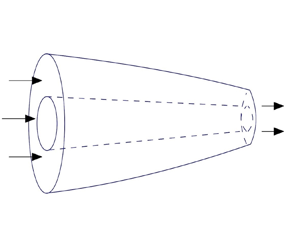
We consider a slender axisymmetric tube of a non-Newtonian fluid with a viscosity that depends on shear rate. This fluid is fed through an aperture of a drawing device with a constant velocity  $U_{in}$ (see figure 1). At the aperture, the outer radius is denoted by $H_{in}$, and the inner radius is denoted by $h_{in}$. We define $\alpha$ to be the ratio of the inner to the outer radius at the input aperture with $0\leq \alpha <1$. At a distance $L$ from the aperture, the tube is pulled by a take-up roller such that the tube has a speed $U_{out}$. In what follows, $z$ is the distance measured along the axis of the tube and $r$ is the distance measured radially outward from the centre of the tube. The inner and outer radii of the tube are denoted by $h(z, t)$ and $H(z,t)$, respectively.

Figure 1. Schematic of the tube-drawing process.
Assuming an incompressible fluid, the governing equations for the conversation of mass and momentum are
 $$\begin{gather} \boldsymbol{\nabla}\boldsymbol{\cdot}\boldsymbol{u}=0, \end{gather}$$
 $$\begin{gather}\rho(\boldsymbol{u}_t+\boldsymbol{u}\boldsymbol{\cdot}\boldsymbol{\nabla}\boldsymbol{u}) =-\boldsymbol{\nabla}p+\boldsymbol{\nabla}\boldsymbol{\cdot}\boldsymbol{\tau}, \end{gather}$$
where  $\rho$ is the density of the fluid and $p$ is the fluid pressure. We denote the velocity as $\boldsymbol {u} = (v, 0, u)$, where $v$,
$v$,  $0$ and $u$ are the velocity components in the $r$,
$r$,  $\theta$ and $z$ direction, respectively. We adopt the rheological model in which the viscous stress tensor is given by
 \begin{equation} \boldsymbol{\tau}=\mu(\varGamma)\dot{\boldsymbol{\gamma}}\quad \text{with}\ \dot{\boldsymbol{\gamma}}=\boldsymbol{\nabla}\boldsymbol{u}+(\boldsymbol{\nabla}\boldsymbol{u})^{\rm T},\end{equation}
where the differential operator is given by  $\boldsymbol {\nabla }=\boldsymbol {e}_r\partial _r+\boldsymbol {e}_\theta \partial _\theta /r+\boldsymbol {e}_z \partial _z$, and $\boldsymbol {e}_r$, $\boldsymbol {e}_\theta$, $\boldsymbol {e}_z$ denote the unit vectors in cylindrical coordinates. The second invariant of the strain-rate tensor is expressed as
 \begin{equation} \varGamma=\tfrac{1}{2}\dot{\boldsymbol{\gamma}}:\dot{\boldsymbol{\gamma}},\end{equation}
and the following power-law model is adopted
 \begin{equation} \mu=K\varGamma^{(n-1)/2},\end{equation}
where  $K$ is the flow consistency index and $n$ is the power-law index that characterises the fluid behaviour. The fluid is shear-thinning for $n<1$, it is shear-thickening for $n>1$ and $n=1$ corresponds to the Newtonian case in which the viscosity is independent of the shear rate. On the inner and outer surfaces of the tube, the dynamic boundary conditions are given by
 $$\begin{gather} \boldsymbol{n}_1\boldsymbol{\cdot}(-p\boldsymbol{I}+\boldsymbol{\tau})\boldsymbol{\cdot}\boldsymbol{n}_1=-\gamma \kappa_1,\quad \boldsymbol{t}_1\boldsymbol{\cdot}(-p\boldsymbol{I}+\boldsymbol{\tau})\boldsymbol{\cdot}\boldsymbol{n}_1=0\quad \text{at}\ r=h(z,t), \end{gather}$$
 $$\begin{gather}\boldsymbol{n}_2\boldsymbol{\cdot}(-p\boldsymbol{I}+\boldsymbol{\tau})\boldsymbol{\cdot}\boldsymbol{n}_2=-\gamma \kappa_2,\quad \boldsymbol{t}_2\boldsymbol{\cdot}(-p\boldsymbol{I}+\boldsymbol{\tau})\boldsymbol{\cdot}\boldsymbol{n}_2=0\quad \text{at}\ r=H(z,t). \end{gather}$$
Here,  $\gamma$ is the surface tension, $\kappa _1$ and $\kappa _2$ are the mean curvatures of inner and outer surfaces, given by
 $$\begin{gather} \kappa_1=\left[\frac{h_{zz}}{(1+(h_z)^2)^{{3}/{2}}}-\frac{1}{h(1+(h_z)^2)^{{1}/{2}}}\right], \end{gather}$$
 $$\begin{gather}\kappa_2=-\left[\frac{H_{zz}}{(1+(H_z)^2)^{{3}/{2}}}-\frac{1}{H(1+(H_z)^2)^{{1}/{2}}}\right]. \end{gather}$$
The vectors  $\boldsymbol {n}_i$ and $\boldsymbol {t}_{i}$ ( $i=1,\ 2$) are the unit vectors on the inner and outer surfaces in the outward and tangential directions, respectively, given by
 $$\begin{gather} \boldsymbol{n}_1=\frac{1}{\sqrt{1+(h_z)^2}}(-1,\ 0,\ h_z),\quad \boldsymbol{n}_2=\frac{-1}{\sqrt{1+(H_z)^2}}(-1,\ 0,\ H_z), \end{gather}$$
 $$\begin{gather}\boldsymbol{t}_1=\frac{1}{\sqrt{1+(h_z)^2}}(h_z,\ 0,\ 1),\quad \boldsymbol{t}_2=\frac{-1}{\sqrt{1+(H_z)^2}}(H_z,\ 0, 1). \end{gather}$$
The kinematic boundary conditions are
 \begin{equation} h_t+uh_z=v\quad \text{at}\ r=h(z,t)\quad \text{and}\quad H_t+u H_z=v\quad \text{at}\ r=H(z,t). \end{equation}
At the entrance and exit, the boundary conditions are
 \begin{equation} u=U_{in}\quad \text{at}\ z=0\quad \text{and}\quad u=U_{out}\quad \text{at}\ z=L.\end{equation}
We adopt the following choices for the scales for non-dimensionalisation:
 \begin{equation} \left.\begin{array}{c@{}} z=Lz^\prime,\quad r=\varepsilon L r^\prime,\quad h=\varepsilon L h^\prime,\quad H=\varepsilon L H^\prime,\quad t=(L/U_{in})t^\prime,\\ u=U_{in}u^\prime,\quad v=\varepsilon U_{in}v^\prime,\quad \mu=K(U_{in}/L)^{n-1} \mu^\prime,\quad p=K(U_{in}/L)^{n} p^\prime,\end{array}\right\} \end{equation}
where  $\varepsilon =(H_{in}\sqrt {1-\alpha ^2})/L$. The quantity $\varepsilon$ represents the square root of the cross-sectional area at the aperture divided by the length of the device and, hence, is a measure of the aspect ratio.
By substituting the scalings in (2.13) into the governing equations and boundary conditions stated in (2.1)–(2.12), we obtain
 $$\begin{gather} u_{z}+\frac{1}{r}(rv)_r=0, \end{gather}$$
 $$\begin{gather}Re\,\varepsilon^2(u_t+uu_z+vu_r)=-\varepsilon^2p_z+2\varepsilon^2(\mu u_z)_z+\frac{1}{r}[r\mu(u_r+\varepsilon^2 v_z)]_r, \end{gather}$$
 $$\begin{gather}Re \,\varepsilon^2(v_t+uv_z+vv_r)=-p_r+[\mu(u_r+\varepsilon^2 v_z)]_z+\frac{2}{r}(r\mu v_r)_r-\frac{2\mu v}{r^2}, \end{gather}$$
and
 \begin{align} &-p+\frac{1}{1+\varepsilon^2 (h_z)^2}[2\mu v_r-2\mu h_z(u_r+\varepsilon^2 v_z)+2\varepsilon^2 (h_z)^2\mu u_z]\nonumber\\ &\quad =\frac{1}{Ca}\left[\frac{1}{h(1+\varepsilon^2 (h_z)^2)^{1/2}}-\frac{\varepsilon^2h_{zz}}{(1+\varepsilon^2 (h_z)^2)^{3/2}}\right]\quad \text{at}\ r=h(z,t), \end{align}
 \begin{align} &-p+\frac{1}{1+\varepsilon^2 (H_z)^2}[2\mu v_r-2\mu H_z(u_r+\varepsilon^2 v_z)+2\varepsilon^2 (H_z)^2\mu u_z]\nonumber\\ &\quad =-\frac{1}{Ca}\left[\frac{1}{H(1+\varepsilon^2 (H_z)^2)^{1/2}}-\frac{\varepsilon^2H_{zz}}{(1+\varepsilon^2 (H_z)^2)^{3/2}}\right]\quad \text{at}\ r=H(z,t), \end{align}
 $$\begin{gather} 2\varepsilon^2h_z\mu v_r-(h_z)^2\mu(\varepsilon^2u_r+\varepsilon^4v_z)+\mu(u_r+\varepsilon^2 v_z)-2\varepsilon^2 h_z\mu u_z=0\quad \text{at}\ r=h(z,t), \end{gather}$$
 $$\begin{gather}2\varepsilon^2 H_z\mu v_r-(H_z)^2\mu(\varepsilon^2u_r+\varepsilon^4v_z)+\mu(u_r+\varepsilon^2 v_z)-2\varepsilon^2H_z\mu u_z=0\quad \text{at}\ r=H(z,t). \end{gather}$$
The non-dimensional viscosity is as follows:
 \begin{equation} \mu=\left(2u_z^2+\frac{1}{\varepsilon^2}u^2_r+\varepsilon^2v^2_z+2u_rv_z+2v^2_r+2\frac{v^2}{r^2}\right)^{(n-1)/2}.\end{equation}
The dimensionless boundary conditions at the entrance and exit are given by
 $$\begin{gather} u=1\quad \text{at}\ z=0, \end{gather}$$
 $$\begin{gather}u={D}\quad \text{at}\ z=1. \end{gather}$$
Here,
 \begin{equation} Re=\left(\frac{U_{in}}{L}\right)^{1-n}\frac{\rho U_{in}L}{K},\quad {Ca}=\left(\frac{U_{in}}{L}\right)^{n-1}\frac{KU_{in}\varepsilon}{\gamma},\quad {D}=\frac{U_{out}}{U_{in}}, \end{equation}
where  $Re$ is the Reynolds number that compares the relative importance of inertial and viscous effects, ${Ca}$ is the capillary number, which quantifies the relative importance of viscous and surface tension forces, and ${D}$ is the draw ratio that represents the ratio of output and input velocities. The kinematic boundary conditions (2.11) remain unchanged under the scaling transformations.
Typical values of the parameters in such flows can vary dramatically depending on the precise nature of the industrial process. This is because the speed of the flow and the viscosity of the materials can vary over many orders of magnitude. In most cases  $\varepsilon$ will be at most $O(10^{-1})$ and can be much smaller. For drawing, ${D}$ is often selected as large as possible and may be of the order of $O(10^3)$ or even larger. On the other hand, extrusion flows may have effective values of ${D}$ much closer to unity (Tronnolone, Stokes & Ebendorff-Heidepriem Reference Tronnolone, Stokes and Ebendorff-Heidepriem2017). Moreover, both small and large ${Re}$ and ${Ca}$ limits can be important (Bechert & Scheid Reference Bechert and Scheid2017). With these factors in mind we will study a broad range of possible parameter values in this paper.
Following the approach used by many previous authors (Fitt et al. Reference Fitt, Furusawa, Monro and Please2001; Wylie et al. Reference Wylie, Huang and Miura2007; Stokes, Bradshaw-Hajek & Tuck Reference Stokes, Bradshaw-Hajek and Tuck2011; He et al. Reference He, Wylie, Huang and Miura2016; Wylie et al. Reference Wylie, Papri, Stokes and He2023), we proceed by assuming  $\varepsilon \ll 1$ and posing the following asymptotic expansions,
 $$\begin{gather} u=u_{0}+\varepsilon^2 u_1+O(\varepsilon^4), \end{gather}$$
 $$\begin{gather}v=v_{0}+\varepsilon^2 v_1+O(\varepsilon^4), \end{gather}$$
 $$\begin{gather}\mu=\mu_{0}+\varepsilon^2 \mu_1+O(\varepsilon^4), \end{gather}$$
 $$\begin{gather}p=p_{0}+\varepsilon^2 p_1+O(\varepsilon^4). \end{gather}$$
For Newtonian fluids, the viscosity  $\mu$ is an order-one quantity. However, in this case, the size of the viscosity depends on the shear rate, as given by (2.21). We note that $\mu$ is $O(\varepsilon ^{-2})$ if $u_{0r}\not \equiv 0$ and $O(1)$ if $u_{0r}\equiv 0$. Nevertheless, one can readily show that assuming $u_{0r}\not \equiv 0$ leads to a contradiction. Hence, $u_0$ is independent of $r$ and so we obtain $u_0\equiv u_0(z,t)$, which is also the case for Newtonian fluids.
Substituting (2.25)–(2.27) into (2.21) and using the fact that  $u_{0r}\equiv 0$, we obtain
 \begin{equation} \mu_0=\left(2u^2_{0z}+\frac{2v_0^2}{r^2}+2v^2_{0r}\right)^{(n-1)/2}.\end{equation}
Furthermore, substituting (2.25)–(2.28) into (2.14) and integrating with respect to  $r$, we obtain the leading-order continuity equation
 \begin{equation} v_0=-\frac{r}{2}u_{0z}-\frac{C(z,t)}{r},\end{equation}
where  $C(z,t)$ is to be determined.
Combining (2.29) with (2.30) yields
 \begin{equation} \mu_0=\left(\frac{4C^2}{r^4}+3u^2_{0z}\right)^{(n-1)/2},\end{equation}
from which it is readily seen that  $\mu _0$ depends on $r$ if $C$ is not identically zero.
The leading-order  $r$-momentum equation (2.16) is
 \begin{equation} p_{0r}=2\mu_{0r}v_{0r}.\end{equation}
Again, we note that  $p_0$ depends on $r$ if $C$ is not identically zero.
At  $O(\varepsilon ^2)$, the tangential stress boundary conditions give
 $$\begin{gather} 2 h_z\mu_0v_{0r}+\mu_0v_{0z}-2 h_z\mu_0u_{0z}+\mu_0u_{1r}=0\quad \text{at}\ r=h(z,t), \end{gather}$$
 $$\begin{gather}2H_z\mu_0v_{0r}+\mu_0v_{0z}-2H_z\mu_0u_{0z}+\mu_0u_{1r}=0\quad \text{at}\ r=H(z,t). \end{gather}$$
The leading-order normal stress boundary conditions give
 $$\begin{gather} -p_0+2\mu_0v_{0r}=\frac{1}{Ca}\frac{1}{h}\quad \text{at}\ r=h(z,t), \end{gather}$$
 $$\begin{gather}-p_0+2\mu_0v_{0r}=-\frac{1}{Ca}\frac{1}{H}\quad \text{at}\ r=H(z,t). \end{gather}$$
In addition, the second-order  $z$-momentum equation (2.15) gives
 \begin{equation} Re(u_{0t}+u_0u_{0z})=-p_{0z}+2(\mu_0u_{0z})_z+\frac{1}{r}(r\mu_0v_{0z})_r +\frac{1}{r}(r\mu_0u_{1r})_r.\end{equation}
Substituting (2.30) and (2.31) into (2.32) and attempting to integrate with respect to  $r$, we see that $p_0$ cannot be expressed in terms of elementary functions (Hazewinkel Reference Hazewinkel1997) unless $C$ is identically zero. This is in direct contrast to the case of a Newtonian tube or the case of a shear-thinning (or shear-thickening) thread with no hole. In both of these cases we obtain $C=0$ and, hence, one can use the fact that $p_0$ and $\mu _0$ are independent of $r$ to integrate (2.37) and use (2.33)–(2.36) to obtain simple long-wavelength evolution equations. In addition, due to the $r$-dependence of $\mu _0$ and $p_0$, one cannot analytically integrate (2.37) to remove the $r$-dependence from (2.37) and (2.33)–(2.36) and obtain leading-order equations with only $z$ and $t$ dependence. This implies that the combination of the hole and the non-Newtonian rheology makes the problem significantly more challenging than the cases of a Newtonian tube or a power-law solid thread.
In order to proceed, we integrate (2.32) by parts to obtain
 \begin{equation} {-}p_0+2\mu_0v_{0r}=2\int \mu_0 v_{0rr}\,{\rm d}r+A(z,t),\end{equation}
where  $A(z,t)$ is an integration function.
Subtracting (2.35) from (2.36) and eliminating  $p_0$ and $v_0$ using (2.30) and (2.38), we obtain an implicit integral equation for $C$
$C$
 \begin{equation} 4C\int_{h}^{H} \frac{1}{r^3}\left(3u_{0z}^2+4\frac{C^2}{r^4}\right)^{{(n-1)}/{2}}\,{\rm d}r =\frac{1}{Ca}\left(\frac{1}{h}+\frac{1}{H}\right).\end{equation}
From (2.30) we see that the radial velocity has two components. The first component  $-r u_{0z}/2$ is induced by the axial stretching and the conservation of mass. The second component $-C/r$ represents a radial strain that is induced by the difference between the surface tension forces on the inner and outer surfaces. In the case of zero surface tension ( ${Ca}=\infty$), this term will be zero. This is clearly reflected in (2.39). In order to proceed further, we consider two approximations of (2.39) that allow us to derive long-wavelength equations.
2.1. Viscosity dominated by the axial strain
Observing (2.39) in the case where the surface tension is weak ( ${Ca}\gg 1$) we expect that $C$ will be small. This means that $3 u_{0z}^2\gg 4C^2/r^4$ and, hence, the viscosity $\mu _0$ will be dominated by axial strain. This will be valid as long as $r$ is not too small and we will return to the validity of the assumption later in § 3. We proceed by posing an asymptotic form
 \begin{equation} C=\frac{1}{Ca} C^{(1)}+\frac{1}{{Ca}^3}C^{(3)} + \cdots.\end{equation}
On substituting (2.40) into (2.39), using the binomial expansion on the bracket in the integral and equating the powers of  $1/{Ca}$, we obtain
 $$\begin{gather} C^{(1)}=\frac{3^{(1-n)/2}u^{1-n}_{0z}h H }{2(H-h)}, \end{gather}$$
 $$\begin{gather}C^{(3)}=-\frac{2(n-1)C^{(1)3}}{9u^2_{0z}}\left(\frac{1}{h^4}+\frac{1}{H^4} +\frac{1}{h^2H^2}\right). \end{gather}$$
 On substituting (2.40) into (2.31) and (2.32), using (2.35)–(2.36), and expanding to order  $O(1/{Ca}^3)$, we obtain
 \begin{align} p_0&=-3^{(1-n)/2}u^n_{0z}+\frac{1}{{Ca}(H-h)}-\frac{2(n-1)3^{(n-3)/2}u^{n-2}_{0z}C^{(1)2}}{{Ca}^2r^4}\nonumber\\ &\quad -\frac{4(n-1)3^{(n-5)/2}u_{0z}^{n-3}C^{(1)3}}{{Ca}^3} \left(\frac{h^2+H^2}{h^4H^4}-\frac{2}{r^6}\right). \end{align}
Furthermore, multiplying (2.37) by  $r$, integrating over $r$, using (2.33)–(2.34), (2.40)–(2.43) and expanding to $O(1/{Ca}^3)$, the following momentum equation is obtained:
 \begin{align} &Re(H^2-h^2)(u_{0t}+u_0u_{0z})=3^{(n+1)/2}[(H^2-h^2)u_{0z}^n]_z+\frac{1}{Ca}(h+H)_z\nonumber\\ &\quad +\frac{1}{{Ca}^2}\left[\frac{3^{(1-n)/2}u^{-n}_{0z}(n-1)(H+h)}{2(H-h)}\right]_z\nonumber\\ &\quad -\frac{4(n-1)3^{(n-5)/2}}{{Ca}^3}(u_{0z}^{n-3}C^{(1)3})_z \left[\frac{H^4-h^4}{h^4H^4}-(H^2-h^2)\left(\frac{h^2+H^2}{h^4H^4}\right)_z\right]\nonumber\\ &\quad -\frac{4}{{Ca}^3}\left(\frac{H_z}{H}-\frac{ h_z}{h}\right)[3^{(n-1)/2}u^{n-1}_{0z}C^{(3)}+2(n-1)3^{(n-3)/2}u^{n-3}_{0z}C^{(1)3}]. \end{align}
Moreover, by substituting (2.30) into the kinematic boundary conditions (2.11) and retaining terms up to  $O(1/{Ca}^3)$, we have
 $$\begin{gather} (h^2)_t+(h^2u_0)_z=-\frac{2 C^{(1)}}{Ca}-\frac{2C^{(3)}}{{Ca}^3}, \end{gather}$$
 $$\begin{gather}(H^2)_t+(H^2u_0)_z=-\frac{2 C^{(1)}}{Ca}-\frac{2C^{(3)}}{{Ca}^3}. \end{gather}$$
The boundary conditions for  $u_0,\ h$ and $H$ are
 $$\begin{gather} u_0=1,\quad h=\frac{\alpha}{\sqrt{1-\alpha^2}},\quad H=\frac{1}{\sqrt{1-\alpha^2}}\quad \text{at}\ z=0, \end{gather}$$
 $$\begin{gather}u_0={D}\quad \text{at}\ z=1. \end{gather}$$
The above system of equations represents a one-dimensional model for a power-law fluid tube, which can be used to study the steady-state profiles and their stability. From (2.45) and (2.46), we see that there is no  $O(1/{Ca}^2)$ correction for $h$ and $H$. Hence, the error in only keeping the $O(1/{Ca})$ terms is of $O(1/{Ca}^3)$. In addition, we note that for the leading order of the asymptotic expansions (2.25)–(2.28) to be consistent with (2.40), we require that $1/{Ca} \gg \varepsilon ^2$.
We note that for a Newtonian fluid ( $n=1$), (2.44)–(2.46) agree with the equations derived by Fitt et al. (Reference Fitt, Furusawa, Monro and Please2001). Moreover, in this case, one can readily see that our expansion is valid for arbitrary ${Ca}$. On the other hand, for a solid thread in which $h(z,t)\equiv 0$, we obtain $C(z,t)\equiv 0$, and hence $\mu _0$ and $p_0$ in (2.31)–(2.32) will be independent of $r$. We can therefore set $h=0$ in (2.44)–(2.46), to obtain the equations for a solid thread that are given by
 $$\begin{gather} Re\,H^2(u_{0t}+u_0u_{0z})=\frac{1}{Ca}\partial_z H+3^{(n+1)/2}(H^2u_{0z}^n)_z, \end{gather}$$
 $$\begin{gather}(H^2)_t+(H^2 u_0)_z=0. \end{gather}$$
The boundary conditions for  $u_0,\ h$ and $H$ are
 $$\begin{gather} u_0=1,\quad H=1\quad \text{at}\ z=0, \end{gather}$$
 $$\begin{gather}u_0={D}\quad \text{at}\ z=1. \end{gather}$$
In this case, one can also readily see that our expansion is also valid for arbitrary  ${Ca}$. Equations (2.49)–(2.52) represent a generalisation that introduces inertial and surface tension effects to the system used by Pearson & Shah (Reference Pearson and Shah1974) and Van der Hout (Reference Van der Hout2000) for an inertialess solid thread with zero surface tension, which has not, to the best of the authors’ knowledge, been considered before.
2.2. Viscosity dominated by the radial strain
We now consider the case in which the radial strain induced by the surface tension will be sufficiently large that the integral in (2.39) will be dominated by the second term in the bracket inside the integral. This will be valid if  $4C^2/r^4\gg 3u_{0z}^2$. From (2.39) we see that this will be the case if either ${Ca}\ll 1$ or if the hole is sufficiently close to closing. We return to the validity of this assumption in § 3.
Since the viscosity is dominated by the radial strain, from (2.29) we obtain the approximation
 \begin{equation} \mu_0=(2C)^{n-1}r^{2-2n}.\end{equation}
By substituting (2.53) into (2.32) and integrating, we can determine the expression for  $p_0$ involving an undetermined function of $z$ and $t$. Subsequently, we utilise (2.35) and (2.36) to uniquely determine $p_0$ and $C$, which are given by
 $$\begin{gather} p_0=-(2C)^{n-1}r^{2-2n}u_{0z}+\frac{2^n}{n}(1-n)C^n r^{-2n}+\frac{h^{2n-1}+H^{2n-1}}{{Ca}(H^{2n}-h^{2n})}, \end{gather}$$
 $$\begin{gather}C=\frac{1}{2}\left[\frac{n(h+H)h^{2n-1}H^{2n-1}}{{Ca}(H^{2n}-h^{2n})}\right]^{1/n}. \end{gather}$$
Furthermore, following a procedure similar to that used in the derivation of (2.44)–(2.46), we obtain
 \begin{align} &Re(H^2-h^2)(u_{0t}+u_0u_{0z})=\frac{2^n}{n}(H^{2-2n}-h^{2-2n})(C^{n})_z +2^n[3(H^{4-2n}-h^{4-2n})C^{n-1}u_{0z}]_z\nonumber\\ &\quad -\frac{(H^2-h^2)}{Ca}\left(\frac{h^{2n-1}+H^{2n-1}}{H^{2n}-h^{2n}}\right)_z -2^{n+1}(H^{1-2n}H_z-h^{1-2n}h_z)C^{n}, \end{align}
and
 $$\begin{gather} (h^2)_t+(h^2 u_{0})_z=-\frac{1}{{Ca}^{1/n}}\left[\frac{n(h+H)h^{2n-1}H^{2n-1}}{(H^{2n}-h^{2n})}\right]^{1/n}, \end{gather}$$
 $$\begin{gather}(H^2)_t+(H^2 u_{0})_z=-\frac{1}{{Ca}^{1/n}}\left[\frac{n(h+H)h^{2n-1}H^{2n-1}}{(H^{2n}-h^{2n})}\right]^{1/n}. \end{gather}$$
Remark In this case, the resulting system (2.56)–(2.58) cannot reduce to the equations for a solid thread. This is because setting  $h=0$ leads to $C^{(0)}=0$, which makes the term $3u^2_{0z}$ dominant. Therefore, even for strong surface tension, the reduced equations of (2.44)–(2.46) are still applicable to a solid thread. On the other hand, we note that for a Newtonian fluid ( $n=1$), (2.56)–(2.58) agree with the equations derived by Fitt et al. (Reference Fitt, Furusawa, Monro and Please2001).
3. Steady-state solutions and their validity
In this section we consider the steady-state solutions of the drawing problem. We note that we have two opposing approximations, the validity of each approximation is considered separately.
3.1. Steady-state solutions when viscosity is dominated by the axial strain
From (2.39) we immediately see that  $C$ will be small in the limit of ${Ca}\ll 1$. In this section we focus on the production of a holey fibre which necessitates the presence of a hole at the exit of the fibre. By evaluating (2.44)–(2.46) in the steady state and truncating the equations at $O(1/{Ca}^2)$, this section provides a detailed analysis of the effects of Reynolds number, capillary number, draw ratio and power-law index on the drawing process and the resulting hole size.
Setting  $\partial _t\equiv 0$ in (2.44)–(2.46) and we obtain
 $$\begin{gather} Re\, u_{0z}=3^{(n+1)/2}[(H^2-h^2)u_{0z}^n]_z+\frac{1}{Ca}(h+H)_z, \end{gather}$$
 $$\begin{gather}(h^2 u_0)_z=-\frac{3^{(1-n)/2}u^{(1-n)}_{0z}hH}{{Ca}(H-h)}, \end{gather}$$
 $$\begin{gather}(H^2 u_0)_z=-\frac{3^{(1-n)/2}u^{(1-n)}_{0z}hH}{{Ca}(H-h)}, \end{gather}$$
with
 $$\begin{gather} u_0=1,\quad h=\frac{\alpha}{\sqrt{1-\alpha^2}},\quad H=\frac{1}{\sqrt{1-\alpha^2}}\quad \text{at}\ z=0, \end{gather}$$
 $$\begin{gather}u_0={D}\quad \text{at}\ z=1. \end{gather}$$
If we consider situations with negligible inertia, we can exploit the fact that we have weak surface tension ( $1/{Ca}\ll 1$) to apply a regular perturbation method and obtain explicit solutions to the leading-order equations for $h,\ H$, and $u_0$, which are given by
 $$\begin{gather} u_{0}=(({D}^{(n-1)/n}-1)z+1)^{n/(n-1)}+O\left(\frac{1}{Ca}\right), \end{gather}$$
 $$\begin{gather}h=\frac{\alpha}{\sqrt{u_0}\sqrt{1-\alpha^2}}+O\left(\frac{1}{Ca}\right), \end{gather}$$
 $$\begin{gather}H=\frac{1}{\sqrt{u_0}\sqrt{1-\alpha^2}}+O\left(\frac{1}{Ca}\right). \end{gather}$$
For the sake of brevity, the details of this calculation, which are straightforward, are omitted. If we take the limit as  $n\to 1$, we note that (3.6)–(3.8) recover the solutions obtained by Fitt et al. (Reference Fitt, Furusawa, Monro and Please2001) in the case of zero surface tension for a tube composed of Newtonian fluids. The solution at the next order cannot be obtained analytically, but the leading-order solution can be used as part of a numerical shooting technique that we describe in § 3.1.1. The leading-order expressions also provide us with a valuable tool to consider the validity of the asymptotic techniques we applied to obtain the solution to (2.39) for ${Ca}\gg 1$.
In the derivation of (2.41)–(2.42) a binomial expansion was employed which required
 \begin{equation} \frac{4 C^2}{3 h^4 u_{0z}^2}\ll1.\end{equation}
With the use of (2.41)–(2.42), (3.6)–(3.8) and (3.9), we can determine the values of  ${Ca}$ for this expansion to remain valid. This requirement is given by
 \begin{equation} Ca\gg\frac{\sqrt{1+\alpha}}{3^{n/2}\alpha\sqrt{1-\alpha}} \left(\frac{n-1}{({D}^{1-1/n}-1)n}\right)^{n}.\end{equation}
This shows that our approximation is difficult to satisfy if  $\alpha$ is small (corresponding to a small inlet hole size) or if $\alpha$ is close to unity (corresponding to a very thin-walled initial tube). In both of these cases the radial strain induced by the surface tension is strong. It is also difficult to satisfy if ${D}$ is close to unity (which corresponds to a draw with minimal stretching). In this case the strain rate associated with the extensional flow induced by the pulling is weak and cannot easily dominate the strain rate associated with the radial strain induced by the surface tension. On the other hand, the condition becomes increasingly less restrictive as ${D}$ becomes large.
3.1.1. Numerical method for steady-state problem
In order to numerically obtain the steady-state solutions, we note that (3.1) is a second-order ordinary differential equation (ODE) for the quantity  $u_0$, and (3.2)–(3.3) are two first-order ODEs for $h$ and $H$. We have three boundary conditions at $z=0$ and one boundary conditions at $z=1$. Therefore, this system can be readily solved using a shooting method in which one needs to guess the value of $u_{0z}$ at $z=0$, then numerically solve (3.1)–(3.3) using a standard ‘initial’ value ODE solver (e.g. MATLAB function ‘ode45’) subject to the ‘initial’ conditions (3.4). Then a root-finding technique (e.g. MATLAB function ‘fsolve’) can be used to find $u_{0z}$ at $z=0$ such that the condition (3.5) is satisfied.
3.1.2. Steady-state solutions with negligible inertia
In this section, we consider how the various parameters affect the steady-state solutions. In figure 2, we show how surface tension affects the solution for a shear-thinning tube with zero inertia and for two different values of  ${D}$. In this case, the results show that the axial velocity $u_0$ is relatively insensitive to ${Ca}$. On the other hand, the outer radius and hole size vary significantly with ${Ca}$ and, as ${Ca}$ decreases, both the outer radius and hole size uniformly decrease. This reflects the fact that surface tension acts to close the hole.

Figure 2. The steady-state profiles against  $z$ for different ${Ca}$ with $Re=0$, $\alpha =0.5$ and $n=0.6$. The draw ratio is ${D}=2.2$ for (a–c), and ${D}=1.4$ for (d,e); (a) and (d) are the axial velocity $u_0$, (b) and (e) are the inner radius and (c) and (f) are the outer radius.
In figure 3, we show the hole size at the exit,  $h(z=1)$, plotted as a function of ${Ca}$ for various values of $n$. This behaviour can be explained by (3.2). As the capillary number ( ${Ca}$) increases, the term $(h^2 u_0)$ decreases with $z$ at a slower rate. Consequently, $h_{out}$ becomes bigger, given that $u_0$ is an increasing function of $z$ and $u_0={D}$ at the exit. In comparison with Newtonian fluids, shear-thinning fluids exhibit greater sensitivity to changes in surface tension, whereas shear-thickening fluids display less sensitivity. As ${Ca}\to \infty$ the curves for different values of $n$ all asymptote to the same value that coincides with the Newtonian case. We see that shear-thinning fluids require larger values of ${Ca}$ than shear-thickening fluids to approach the asymptote.

Figure 3. The hole size at the exit, denoted by  $h_{out}$, is plotted against the capillary number ${Ca}$ on a logarithmic scale with ${D}=5$, ${Re}=0$ and $\alpha =0.6$. The inlet hole size is $0.75$. If ${Ca}\to \infty$, $h_{out}$ is independent of $n$ and is given by $h_{out}=\alpha /\sqrt {{D}(1-\alpha ^2)}\approx 0.3354$.
In figure 4, we plot the hole size at the exit as a function of draw ratio for different values of  $n$. Unsurprisingly, we see that the hole size at the exit decreases with increasing draw ratio. However, surprisingly, for small values of ${D}$ we see that the hole size at the exit decreases with increasing $n$ whereas the opposite occurs for larger values of ${D}$. Moreover, there appears to be a special value of ${D}$ for which the hole size at the exit is independent of $n$. This special value is shown as a dashed vertical line. In order to understand this surprising phenomenon, we plot the profiles of $u_0$, $h$ and $H$ in figure 5 for negligible inertia. We choose two values of ${D}$, one above the special value of ${D}$ (figure 5a–c) and one below the special value of ${D}$ (figure 5d–f). This phenomenon can be elucidated by examination of (3.2) and figure 5. In figure 5(a,d) we plot the velocity profile for different values of $n$. We also plot a straight line passing through $u_0=1$ at $z=0$ and $u_0={D}$ at $z=1$ with slope of ${D}-1$. We can see from these figures that for sufficiently small values of the draw ratios, $u_0$ can be roughly approximated by such a straight line (see figure 5d). Under this rough approximation we obtain $u_{0z}={D}-1$. By examining (3.2) we see that the only dependence on $n$ in closing of the hole appears as $(\sqrt {3}u_{0z})^{n-1}$ which we can approximate as $(\sqrt {3}({D}-1))^{n-1}$. Hence, there are two different types of behaviour depending on whether $\sqrt {3}({D}-1)$ is greater or less than unity. Hence, if ${D}<1+1/\sqrt {3}$, $h$ will decrease with increasing $n$, as shown by figures 4 and 5(e). For ${D}=1.8$, figure 5(b) shows that $h$ decreases with increasing $n$ for sufficiently small $z$, but increases with increasing $n$ for larger $z$. This is because $u_{0z}<{D}-1$ for sufficiently small $z$, whereas $u_{0z}>{D}-1$ for larger $z$. The overall effect is that $h$ increases with larger $n$ near the exit, which is consistent with the phenomenon observed by figure 4 above ${D}=1+1/\sqrt {3}$. Despite the somewhat rough nature of the approximation, we obtain remarkable agreement for the special value of ${D}=1+1/\sqrt {3}$ with numerical simulations. Similar arguments explain the phenomena in figure 5(c,f). This special value of ${D}$ is much smaller than what is typically used for the drawing of fibres, but is of comparable size to the values of ${D}$ encountered in extrusion flows.

Figure 4. The hole size at the exit, denoted by  $h_{out}$, is plotted against the draw ratio ${D}$ for different $n$,
$n$,  ${Ca}=15$, $\alpha =0.6$ and $Re=0$. The inlet hole size is $0.75$.

Figure 5. The steady-state profiles against  $z$ for different $n$ with $Re=0$, $\alpha =0.5$ and ${Ca}=15$. The draw ratio is ${D}=1.8$ for (a–c), and ${D}=1.4$ for (d–f); (a) and (d) are the axial velocity $u_0$, (b) and (e) are the inner radius and (c) and (f) are the outer radius.
3.1.3. Steady-state solutions with inertia
Figure 6 shows how inertia affects the behaviour of a tube. As the Reynolds number ( $Re$) increases the thinning of the tube becomes more localised towards the exit at $z=1$. This localisation near the pulled end at $z=1$ occurs because inertia makes it more difficult for the thread to accelerate (and, hence, thin) over the bulk of the device.

Figure 6. The steady-state profiles against  $z$ for different $Re$ with $n=0.6$, $\alpha =0.6$, ${Ca}=15$ and ${D}=1.5$: (a) axial velocity $u_0$; (b) inner radius; (c) outer radius.
Figure 7 illustrates how the hole size  $h$ at the exit varies against $n$ with the Reynolds number. For sufficiently small values of $n$,
$n$,  $h_{out}$ at the exit increases as $Re$ increases, while for sufficiently large values of $n$,
$n$,  $h_{out}$ at the exit decreases with increasing $Re$. This phenomenon can be explained by (3.2) and figure 6(a). As demonstrated in figure 6(a), $u_{0z}$ first decreases with increasing $Re$ for sufficiently small values of $z$, and then increases with increasing $Re$ for sufficiently large values of $z$. Consequently, based on (3.2) and considering the characteristics of the shear-thinning fluid, we observe that $h^2u_0$ with $Re=2$ decreases more slowly than $h^2u_0$ with $Re=0$, and then $h^2u_0$ with $Re=2$ decreases more rapidly than $h^2u_0$ with $Re=0$. The combined effect of these two trends for $h^2u_0$ determines the hole size at the exit. When $n$ is smaller than the value corresponding to the intersection point of the lines with $Re=0$ and $Re=2$ in figure 7, the first trend exerts a dominant influence on the hole size at the exit, as depicted in figure 8(a). However, as $n$ increases, the second trend becomes dominant in determining $h_{out}$, as illustrated in figure 8(b). Furthermore, in the case of larger $n$ (shear-thickening behaviour), the value of $h_{out}$ with $Re=0$ is consistently smaller than that with non-zero $Re$.
$Re$.

Figure 7. The hole size at the exit, denoted by  $h_{out}$, plotted against $n$ for different $Re$,
$Re$,  ${Ca}=15$, $\alpha =0.6$ and ${D}=1.5$. The inlet hole size is $0.75$.

Figure 8. Plot of  $h^2 u_0$ against $z$ for different $Re$,
$Re$,  ${Ca}=15$, $\alpha =0.6$ and ${D}=1.5$: (a) $n=0.6$ and (b) $n=0.9$.
3.2. Steady-state solutions when viscosity is dominated by the radial strain
We now consider the steady-state solutions of (2.56)–(2.58). At first glance this appears to be a complicated nonlinear coupled system of ODEs. However, it can be dramatically simplified using the following transformations. In the steady state, we can use (2.57) and (2.58) along with the boundary conditions (2.47) to see that
 \begin{equation} (H^2-h^2)u_0\equiv1.\end{equation}
Taking  $P=h^2 u_0$, and defining a new independent variable $\eta$ using
 \begin{equation} \frac{{\rm d}\eta}{{\rm d}z}={Ca}^{-1/n}h^{(2n-1)/n}\quad \text{with}\ \eta(0)=0, \end{equation}
we can represent (2.57) in the form
 \begin{equation} \frac{{\rm d}P}{{\rm d}\eta}=-n^{1/n}F(P)\quad \text{with}\ P(0)=\frac{\alpha^2}{1-\alpha^2},\end{equation}
where
 \begin{equation} F(P)=\left[\frac{(\sqrt{1+P}+\sqrt{P})(1+P)^{n-1/2}}{(1+P)^n-P^n}\right]^{1/n}.\end{equation}
Equation (3.13) is a separable equation for  $P(\eta )$ that is decoupled from the velocity. It can be seen that $P$ starts from $\alpha ^2/(1-\alpha ^2)$ at $\eta =0$ and decreases since the right-hand side of (3.13) is negative. Moreover, physical constraints imply that $P$ is always positive. Thus, $F(P)$ in (3.14) is always bounded and tends to $1$ when $P\to 0$.
We next make the transformation
 \begin{equation} q=u_0^{-1/2},\end{equation}
under which the steady-state version of (2.56) is given by
 \begin{align} &Re\,Ca (q^{-2})_{\eta}=[(1+P)^{1-n}-P^{1-n}][(F^n P^{(2n-1)/2})_{\eta}q-2F^n P^{(2n-1)/2}q_{\eta}]\nonumber\\ &\quad -4 n^{(n-1)/n}[3((1+P)^{2-n}-P^{2-n}) F^{n-1} P^{(2n-1)/2}q_{\eta}]_{\eta}\nonumber\\ &\quad -q\left[\frac{P^{(2n-1)/2}+(1-P)^{(2n-1)/2}}{(1+P)^n-P^n}\right]_{\eta} +q_{\eta}\left[\frac{P^{(2n-1)/2}+(1-P)^{(2n-1)/2}}{(1+P)^n-P^n}\right]\nonumber\\ &\quad -F^nP^{(2n-1)/2}\left[2n((1+P)^{1-n}-P^{1-n})q_{\eta} -\frac{n}{1-n}((1+P)^{1-n}-P^{1-n})_{\eta}q\right]. \end{align}
We note that the product  $Re\,{Ca}$ represents the relative importance of inertial to surface tension forces. Moreover, in the limit $Re\,{Ca}\to 0$, (3.16) is a linear ODE for $q$.
$q$.
We next consider the process of hole closure represented by  $h\to 0$ or $P\to 0$. By employing separation of variables and integrating (3.13), we can obtain the location of hole closure, denoted as $\eta _0$. Next, we focus on the behaviour of $P$ and $u_0$ near $\eta _0$. As $\eta$ approaches $\eta _0$, $F\to 1$ and $P\to 0$, and we can see from (3.13) that
 \begin{equation} P=n^{1/n}(\eta_0-\eta)\quad \text{as}\ \eta\to \eta_0.\end{equation}
By substituting (3.17) into (3.16), we can derive the following approximate equations for different ranges of  $n$ when $\eta$ is near $\eta _0$.
If  $n<3/2$, (3.16) can be approximated by
 \begin{equation} Re\,Can^{3/(2n)-2}(\eta_0-\eta)^{3/2-n}(q^{-2})_{\eta}=12(n-\tfrac{1}{2})q_{\eta} -12(\eta_0-\eta)q_{\eta\eta}.\end{equation}
When  $Re=0$, the exact solution to (3.18) is
 \begin{equation} q=B_1(\eta_0-\eta)^{3/2-n}+B_2\quad \text{as}\ \eta\to\eta_0,\end{equation}
where  $B_1$ and $B_2$ are constants to be determined. Upon substituting (3.19) into the inertial term of (3.18), we find that the inertial term remains negligible. Thus, the asymptotic hole closure behaviour described by (3.19) is valid even for non-zero $Re$.
$Re$.
Near  $\eta _0$, the expression for $u_0$ can be obtained by using (3.15) and (3.19) and expanding with respect to $(\eta _0-\eta )$, to give
 \begin{equation} u_0=B_3 (\eta_0-\eta)^{3/2-n}+B_4\quad \text{as}\ \eta\to\eta_0,\end{equation}
where  $B_3$ and $B_4$ are the constants that depend on $B_1$ and $B_2$.
Further, using (3.20) and the fact that  $P=h^2 u_0$, we obtain
 \begin{equation} h^2\sim (\eta_0-\eta)\quad \text{as}\ \eta\to\eta_0,\end{equation}
where the symbol ‘ $\sim$’ represents the same order.
Substituting (3.21) into (3.12) and integrating, we obtain
 \begin{equation} z-z_0\sim-{Ca}^{1/n}(\eta_0-\eta)^{1/(2n)}.\end{equation}
Here,  $z_0$ is the location of hole closure and depends on $\eta _0$. In addition, we assume that $0< z_0<1$, meaning that hole closure occurs within the physical size of the device. Combining (3.21) and (3.22), we obtain
 \begin{equation} h\sim \frac{1}{Ca} (z_0-z)^{n}.\end{equation}
Combining (3.20) and (3.22), we obtain
 \begin{equation} u_0\sim \frac{B_3}{{Ca}^{3-2n}}(z_0-z)^{3-2n}+B_4.\end{equation}
We recall that the derivation of (2.56)–(3.13) requires that the viscosity is dominated by the radial strain and, hence,  $4 C^2/r^4\gg 3 u_{0z}^2$. In the limit $h\to 0$, $C$ can be approximated by
 \begin{equation} C=\frac{n^{1/n}h^{2-1/n}}{2{Ca}^{1/n}}.\end{equation}
Thus, the validity of this approximation (2.53) requires
 \begin{equation} h\ll \frac{n}{3^{n/2}u^n_{0z} {Ca}}.\end{equation}
Using (3.23) and (3.24) it is straightforward to check that this will be satisfied for  $n<3/2$ as hole closure is approached. Therefore, (2.56)–(2.58) will be valid in the limit $h\to 0$ for $n<3/2$ and automatically violated if $n\geq 3/2$. On the other hand, if we do not consider hole closure, then (3.26) simply requires that ${Ca}\ll 1$.
For  $n\geq 3/2$, the details are complicated, but one can show that the solution of (3.16) gives a velocity that diverges to infinity as hole closure is approached. This behaviour occurs for both $Re\, {Ca}=0$ and $Re\, {Ca}\neq 0$. In this case, the assumption that the viscosity is dominated by radial strain fails and, hence, this solution is not appropriate to describe hole closure. For $n\geq 3/2$, it hence seems natural to consider hole closure in the opposite limit in which the viscosity is dominated by axial strain and we obtain (2.44)–(2.46). Nevertheless, one can show that the assumption $2C/(\sqrt {3} h^2 u_{0z})\ll 1$ used to derive (2.44)–(2.46) is also invalid in the limit as hole closure occurs. Since hole closure cannot occur in either of the two limits, we postulate that hole closure cannot occur for $n\geq 3/2$.
4. Linear stability
In this section, we carry out linear stability analysis to determine the critical value of the draw ratio (that we denote by  ${D}_{c}$) for which draw resonance instability occurs. We also determine how the instability is affected by inertia, surface tension, the power-law index and the inlet hole size. In § 2 we derived two different sets of equations: (2.44)–(2.46) that are valid for ${Ca}\gg 1$ as long as the hole does not approach closure; and (2.56)–(2.58) that are valid near hole closure. Since (2.56)–(2.58) mainly describe the hole closure phenomenon, they will typically not be able to describe the full stretching dynamics. We therefore only focus on the stability of (2.44)–(2.46). To investigate the linear stability, we denote the steady-state profiles in § 3 as $\hat {u}_0(z),\ \hat {h}(z)$ and $\hat {H}(z)$ and add small perturbations of the form $\textrm {e}^{\lambda t}\tilde {u}_0(z)$, $\textrm {e}^{\lambda t}\tilde {h}(z)$ and $\textrm {e}^{\lambda t}\tilde {H}(z)$ to obtain
 $$\begin{gather} u_0(t,z)=\hat{u}_0(z)+\exp(\lambda t)\tilde{u}_0(z), \end{gather}$$
 $$\begin{gather}h(t,z)=\hat{h}(z)+\exp(\lambda t)\tilde{h}(z), \end{gather}$$
 $$\begin{gather}H(t,z)=\hat{H}(z)+\exp(\lambda t)\tilde{H}(z), \end{gather}$$
where  $\lambda$ denotes the growth rate of perturbations.
After substituting into (2.44)–(2.46) with a truncation error of  $O(1/{Ca}^2)$ and linearising in the small perturbations, we obtain
 \begin{align} &Re(\hat{H}^2-\hat{h}^2)[\lambda\tilde{u}_0+\hat{u}_{0z}\tilde{u}_0+\hat{u}_0\tilde{u}_{0z}] -3^{(n+1)/2}n\left[\frac{\hat{u}^{n-1}_{0z}}{\hat{u}_0}\tilde{u}_{0z}\right]_z +2Re[\hat{u}_{0}\hat{u}_{0z}(\hat{H}\tilde{H}-\hat{h}\tilde{h})]\nonumber\\ &\quad -\frac{1}{Ca}(\tilde{h}_z+\tilde{H}_z)-3^{(n+1)/2}[\hat{u}_{0z}(2\hat{H}\tilde{H} -2\hat{h}\tilde{h})]_z=0, \end{align}
 \begin{align} &2\lambda\hat{h}\tilde{h}+(\hat{h}^2\tilde{u}_0)_z+2(\hat{h}\hat{u}_0\tilde{h})_z -\frac{(1-n)3^{(1-n)/2}}{{Ca}(\hat{h}-\hat{H})}\hat{h}\hat{H}\hat{u}^{-n}_{0z}\tilde{u}_{0z} -\frac{3^{(1-n)/2}}{{Ca}(\hat{h}-\hat{H})}\hat{u}^{1-n}_{0z}(\hat{h}\tilde{H} +\hat{H}\tilde{h})\nonumber\\ &\quad +\frac{(1-n)3^{(1-n)/2}}{{Ca}(\hat{h}-\hat{H})^2}\hat{h}\hat{H}\hat{u}^{1-n}_{0z}(\tilde{h}-\tilde{H})=0, \end{align}
 \begin{align} &2\lambda\hat{H}\tilde{H}+(\hat{H}^2\tilde{u}_0)_z+2(\hat{H}\hat{u}_0\tilde{H})_z -\frac{(1-n)3^{(1-n)/2}}{{Ca}(\hat{h}-\hat{H})}\hat{h}\hat{H}\hat{u}^{-n}_{0z}\tilde{u}_{0z}\nonumber\\ &\quad -\frac{3^{(1-n)/2}}{{Ca}(\hat{h}-\hat{H})}\hat{u}^{1-n}_{0z}(\hat{h}\tilde{H} +\hat{H}\tilde{h})+\frac{(1-n)3^{(1-n)/2}}{{Ca}(\hat{h}-\hat{H})^2}\hat{h}\hat{H}\hat{u}^{1-n}_{0z} (\tilde{h}-\tilde{H})=0. \end{align}
The boundary conditions are given by  $\tilde {u}_0=0,\ \tilde {h}=0,\ \tilde {H}=0$ at $z=0$ and $\tilde {u}_0=0$ at $z=1$. Equations (4.4)–(4.6) represent an eigenvalue problem for the growth rate $\lambda$.
4.1. Numerical method for linear stability
In order to solve the above problem, we applied central finite differences to discretise (4.4)–(4.6). This reduces the stability problem to a matrix eigenvalue problem (Wylie et al. Reference Wylie, Papri, Stokes and He2023) that can be solved by standard linear algebra routines. Given a sufficiently large number of grid points, this provides a good estimate for the eigenvalue spectrum of the operator. We are only interested in the eigenvalue with the largest real part and the corresponding eigenfunction. In order to verify the results of our finite difference method, we also applied a shooting technique by guessing the complex value of  $\lambda$. For shooting, one has to be careful in ensuring that one has a good initial guess for $\lambda$. We can obtain an excellent guess from our finite difference method. Using a standard ODE solver (e.g. MATLAB function ‘ode45’), we numerically solved the eigenvalue problem (4.4)–(4.6) subject to the ‘initial’ conditions $\tilde {u}_0=0$, $\tilde {h}=0$, $\tilde {H}=0$ and $\tilde {u}_{0z}=1$ at $z=0$. We then used a rooting-finding technique (e.g. MATLAB function ‘fsolve’) to select $\lambda$ such that the result can match the boundary condition $\tilde {u}_0=0$ at $z=1$. Note that the condition $\tilde {u}_{0z}=1$ is arbitrary since the eigenvalue problem is linear.
4.2. Results of linear stability
The effect of surface tension on the stability is depicted by figure 9, which shows that smaller surface tension (larger  ${Ca}$) makes the flow more stable for all three types of fluid (shear-thinning, Newtonian and shear-thickening fluid). We observe that changes in ${Ca}$ have a weaker relative effect on ${D}_c$ for the shear-thinning case than the shear-thickening case.

Figure 9. The critical draw ratio as a function of  ${Ca}$ for $Re=0$ and $\alpha =0.6$: (a) $n=0.6$, (b) $n=1$ and (c) $n=1.2$.
We further examine the role played by the inlet hole size and  $n$ in figure 10. It shows that the larger the inlet hole size, the more unstable the flow for finite ${Ca}$. In addition, the fluid becomes more stable as $n$ increases. However, in figure 11 we see that the stability is completely independent of the inlet hole size in the limit ${Ca}\to \infty$, the results of ${Ca}=10$ are also presented for comparison. The stability results for the tube are identical to the stability ones in the limit in which surface tension is negligible.

Figure 10. The critical draw ratio as a function of  $n$ for various $\alpha$ with $Re=0$ and ${Ca}=10$. Note that $\alpha =0$ corresponds to a solid thread.

Figure 11. The critical draw ratio as a function of  $\alpha$ for various ${Ca}$ with $Re=0$ and $n=0.6$.
In figure 12, for three types of fluid (shear-thinning fluid, Newtonian fluid and shear-thickening fluid), we examine the role played by inertia on draw resonance for a solid thread and an axisymmetric tube. For all three fluid types, and for both a thread and a tube, increasing the Reynolds number stabilises the flow. In addition, in all cases, for a large enough Reynolds number, the flow becomes unconditionally stable, that is, it is stable for all values of the draw ratio  ${D}$. As $n$ increases, a larger $Re$ is needed to achieve unconditional stability. For Newtonian fluids, this instability mechanism has been investigated carefully by Bechert & Scheid (Reference Bechert and Scheid2017) for a solid thread, and by Wylie et al. (Reference Wylie, Papri, Stokes and He2023) for threads with internal holes. They argued that the instability is driven by a mechanism in which a small increase in the cross-sectional area near the exit leads to an increase in the tension in the thread. This increased tension is transmitted upstream and causes the thread to thin more rapidly near the entrance. This thinner portion of the thread is then advected towards the exit and, hence, causes a decrease in the cross-sectional area near the exit. This represents a half-cycle of the instability. Here, we explore how shear-thinning and shear-thickening affect this instability mechanism. By integrating (2.44), we observe that the effects of inertia reduce the transmission of the tension force upstream towards the entrance. Consequently, inertia has the effect of making flows more stable. This can be seen in the eigenfunctions for $Re=0$ and $Re=0.4$ that are plotted in figure 13. We have normalised the eigenfunctions so that the perturbation to the cross-sectional area at the exit is unity. In the case with larger inertia, the perturbation to the cross-sectional area at the exit leads to less thinning near the entrance and so the inertia has acted to stabilise the flow. In addition, the eigenfunctions for different $n$ are shown in figure 14. For $n=0.9$ we get less thinning throughout the device and, hence, the mechanism of advecting the disturbance is less effective than for $n=0.6$, which explains the behaviour we observed in figure 10.

Figure 12. The real part of the most unstable eigenvalue as a function of the draw ratio  ${D}$ for a tube with $\alpha =0.6$ (solid line) and a solid thread (dashed line): (a) shear-thinning $n=0.6$, (b) Newtonian $n=1$, (c) shear-thickening $n=1.2$, for various values of $Re$ and ${Ca}=10$.

Figure 13. The eigenfunction for different  $Re$ with ${Ca}=15$, $\alpha =0.6$, $n=0.9$ and ${D}=20$: (a) $Re=0$ (blue lines); (b) $Re=0.4$ (red lines). The dashed line represents the imaginary part, whereas the solid line represents the real part.

Figure 14. The eigenfunction for different  $n$ with $Re=0,\ {Ca}=10,\ \alpha =0.5,$ and ${D}=5$: (a) $n=0.6$ (blue lines); (b) $n=0.9$ (red lines). The dashed line represents the imaginary part, whereas the solid line represents the real part.
5. Conclusions
In this paper, we have investigated the steady-state behaviour and stability analysis of the drawing process for a slender tube composed of either shear-thinning or shear-thickening fluid with  $n$ as the power-law index. Our analysis takes into account surface tension and inertial effects. Despite the inherent complexity of this problem, we have demonstrated that by employing asymptotic techniques and making appropriate assumptions, we can dramatically simplify the problem. Specifically, we have obtained a one-dimensional leading-order system for the case of weak surface tension as long as the hole does not approach closure. Using these equations, we have obtained steady-state profiles that reveal several noteworthy phenomena. First, in the case of negligible inertia and a fixed hole size, the hole size at the exit increases with decreasing $n$ when ${D}<1+1/\sqrt {3}$ and decreases with decreasing $n$ when ${D}>1+1/\sqrt {3}$. Second, for a fixed input hole size, the relationship between the hole size at the exit is an increasing function of $Re$ for sufficiently large $n$ and a decreasing function of $Re$ for sufficiently small $n$. Third, for shear-thinning fluids, the hole size at the exit is more sensitive to changes in surface tension than the Newtonian case. For shear-thickening fluids, the hole size at the exit is less sensitive to changes in surface tension. Most polymeric materials that can be used in applications of this type are shear-thinning. Hence, for the large values of ${D}$ that are typical in fibre drawing, the shear-thinning behaviour will cause the hole to close more rapidly than for Newtonian fluids. This is typically deemed to be undesirable and so this can be regarded as a disadvantage of shear-thinning fluids when compared with Newtonian fluids in the case of rapid drawing. On the other hand, for extrusional flows in which the values of ${D}$ are much lower, shear-thinning behaviour may be able to make the hole at the exit larger than the comparable Newtonian flows. This represents an important finding especially because capillary effects tend to be more important in extrusional flows than drawing flows.
We also derived an alternative set of equations that describe hole closure. We obtained the asymptotic forms for the hole size and velocity as closure is approached for  $n<3/2$. On the other hand, if $n\geq 3/2$ the equations become invalid as hole closure is approached, because the axial strain dominates the radial strain in the viscosity. However, if we use the equations for which the axial strain dominates the viscosity, we also found that these equations are invalid as hole closure is approached. We therefore postulate that hole closure cannot occur if $n\geq 3/2$.
Furthermore, we performed a linear stability analysis, which provides insights into the relationship between the critical draw ratio and various factors, including inertia, surface tension, inlet hole size and  $n$. Decreasing surface tension, reducing the hole size and increasing the Reynolds number act to stabilise the flow. Moreover, compared with shear-thinning fluids, Newtonian fluids exhibit greater stability, whereas shear-thickening fluids are even more stable. Consequently, the shear-thinning fluids require a lower Reynolds number to achieve unconditional stability, the shear-thickening fluids require a higher Reynolds number to achieve unconditional stability. In applications, shear thinning is therefore unhelpful in that it makes the critical draw ratio smaller. This will certainly be important for the drawing of optical fibres for which one typically wants to choose ${D}$ to be as large as possible. On the other hand, for extrusional flows the typical values of ${D}$ used are still below the critical ${D}$ we find. Therefore, stability issues are unlikely to be problematic. Overall, shear-thinning materials hence offer some important potential advantages over Newtonian fluids for extrusional flow with sufficiently small ${D}$.
Funding
J.J.W. was supported by the Research Grants Council of Hong Kong Special Administrative Region, China (CityU 11309422).
Declaration of interests
The authors report no conflict of interest.


 Open access