


1. Introduction
Well-defined property rights over land are crucial for economic development (Demsetz, Reference Demsetz1967; North and Thomas, Reference North and Thomas1973). The linkages between land rights, efficiency and economic development have been the subject of much research (e.g., Feder and Feeny, Reference Feder and Feeny1991; Deininger, Reference Deininger2003; Galiani and Schargrodsky, Reference Galiani and Schargrodsky2011; De Janvry et al., Reference De Janvry, Emerick, Gonzalez-Navarro and Sadoulet2015). Such issues are of special interest in a country like China that has seen significant changes in agricultural markets and land rights over the last few decades (e.g., Lin, Reference Lin1992; Rozelle and Li, Reference Rozelle and Li1998). China's rapid growth in agricultural productivity since the 1980s has been associated in part with its successful land reforms (Fan, Reference Fan1991; Lin, Reference Lin1992; Sun et al., Reference Sun, You and Muller2018). Functioning factor markets (including land and labor markets) make it possible for a rural household to delink its labor from on-farm activities and reallocate some labor to off-farm opportunities both locally and remotely (e.g., through migration). For example, with a well-functioning land rental market, households with labor constraints could choose to rent out their farmland to release household labor from on-farm activities.
As a rural economy transitions away from agricultural activities toward other sectors, significant adjustments and economic challenges arise for the farm sector (de Brauw et al., Reference de Brauw, Huang and Rozelle2000; Bowlus and Secular, Reference Bowlus and Secular2003; Adamopoulos et al., Reference Adamopoulos, Brandt, Leight and Restuccia2017). On the one hand, off-farm activities allow the households to diversify income sources, to overcome credit constraints, and to increase the use of industrial inputs (Wang et al., Reference Wang, Wailes and Cramer1996; Rozelle et al., Reference Rozelle, Taylor and de Brauw1999; Taylor et al., Reference Taylor, Rozelle and de Brauw2003). On the other hand, off-farm employment reduces the labor supply to farm production, which may lead to a decreased production efficiency, especially when hired labor is less efficient or exhibits higher moral hazard risk than family labor (e.g. Allen and Lueck, Reference Allen and Lueck1998). As labor moves out of agriculture, the growth of the non-agricultural economy and off-farm labor markets stimulates the demand for land transfers (Kung, Reference Kung2002). In this context, a well-functioning land rental market is helpful in realizing potential gains in household productivity and efficiency (Benjamin and Brandt, Reference Benjamin and Brandt2002).
Starting in the late 1970s and early 1980s, rural land arrangements in China changed from a collectively-owned land system with centrally-planned production to the so-called Household Responsibility System (HRS). With HRS, individual farmers became residual income claimants with land-use rights. Such a change has been considered one of the major factors in China's economic miracle since the early 1980s. Initially households' land-use rights were offered for a duration of 15 years, but in 1993 they were extended for another 30 years after the expiration of the then-current land contracts between village households and the village committee. In 2017, another 30-year extension was granted in the 19th National Congress of the Communist Party of China. In addition, the Chinese government in 2014 decided to complete the land title (contracting right) confirmation in five years. By the end of June 2018, land titling of 1.39 billion mu Footnote 1 (229 million acres) had been completed.Footnote 2
In the face of massive rural migration, land rentals offer great potential to improve agricultural productivity and efficiency by redistributing land toward more efficient farmers (Deininger and Jin, Reference Deininger and Jin2005; Deininger et al., Reference Deininger, Jin, Xia and Huang2014; Adamopoulos et al., Reference Adamopoulos, Brandt, Leight and Restuccia2017). But achieving these benefits requires properly functioning factor markets. The presence of imperfections in both the labor market and the land rental markets makes the evaluation of the effects of Chinese land reform difficult (Kimura et al., Reference Kimura, Otsuka and Rozelle2011; Zhang et al., Reference Zhang, Wang, Glauben and Brummer2011). Chari et al. (Reference Chari, Liu, Wang and Wang2017) report that land right reforms have increased agricultural productivity in China by 7 per cent. Yet, Ma et al. (Reference Ma, Heerink, Geng and Shi2017) find that land certification has negative effects on technical efficiency in Northwest China, and Zhou et al. (Reference Zhou, Shi, Heerink and Ma2019) report that annual and open-ended land transfer contracts have negative impacts on technical efficiency in Eastern China.
These contrasting results are puzzling. They suggest a need to take a new look at the effects of land rental markets on the efficiency and productivity of Chinese rural households. We argue that the ambiguity of previous findings are related to four issues: (1) the need to distinguish between technical and allocative efficiency; (2) the need to investigate efficiency in a multi-output context; (3) the need to control for environmental conditions in efficiency analysis; and (4) the need to control for endogeneity issues. This paper addresses these four issues.
Our first issue is the need to go beyond technical efficiency and to investigate the possible role of allocative efficiency. China's economic reforms have been in the direction of a market economy, indicating that the response of farmers to market signals is a potentially important part of the evaluation of land tenure reform. We see the neglect of allocative efficiency as a significant weakness of previous research for two reasons. First, we expect the rise of land rentals to provide new flexibilities to the functioning of agricultural markets in China. Second, improvements in technical efficiency and allocative efficiency both contribute to increasing income. This raises the question: if land tenure reforms stimulate the agricultural economy, how much of the effects come from technical efficiency versus allocative efficiency? As discussed below, our investigation provides an answer to this question.
Previous analyses have often focused on the linkages between land tenure and technical efficiency in the context of a single-output production function (e.g., Zhang et al., Reference Zhang, Wang, Glauben and Brummer2011; Ma et al., Reference Ma, Heerink, Geng and Shi2017; Zhou et al., Reference Zhou, Shi, Heerink and Ma2019). These studies identify whether land tenure reforms have shifted the production frontier. Farms are typically multi-output enterprises. This supports our second issue: evaluating the efficiency farm households need to include the role of farm output mix, which requires using a multi-input multi-output approach. In contrast to previous analyses, our investigation of both technical and allocative efficiency relies on a multi-input multi-output approach. The third issue (the need to control for environmental conditions) has been stressed by Sherlund et al. (Reference Sherlund, Barrett and Adesina2002) who showed how the neglect of environmental factors can have drastic effects on efficiency estimates. The fourth issue (endogeneity) is also important as endogeneity bias can affect the validity of efficiency estimates. As discussed below, these issues are all addressed explicitly in our analysis.
The goal of this article is to present a refined analysis of the efficiency of rural households and to obtain new insights into the effects of land tenure reform in China. Based on 2009 farm household survey data from three provinces in China, we estimate both technical efficiency and allocative efficiency and their determinants. The data provide us with an opportunity to evaluate the role of factor markets and land arrangements in rural China. Our analysis is applied at the household level, including both farm and off-farm activities. The inclusion of non-farm activities is motivated by the importance of off-farm income for many rural households.
As indicated above, our paper examines the linkages between land rentals and both technical efficiency and allocative efficiency. It relies on a multi-input multi-output analysis that takes into consideration the presence of heterogeneous agro-climatic conditions both across provinces and across farms. The technical efficiency estimates measure productivity levels. Going beyond productivity estimates, our analysis also estimates allocative efficiency, providing useful information on the managerial ability of each household to respond to market conditions. We then proceed with evaluating econometrically the determinants of technical and allocative efficiency, with a focus on the role of land rental activities.
The econometric analysis uses a control function approach to deal with potential endogeneity issues. We find that participation in the land rental market does not affect technical efficiency but has large positive effects on allocative efficiency. This result stresses the need to distinguish between technical and allocative efficiency in the economic analysis of land tenure arrangements. Since higher allocative efficiency improves household income, our analysis shows that land rental transfers contribute to significant increases in household income in rural China.
The paper is organized as follows. Section 2 reviews the conceptual measurement of efficiency. The analysis relies on output-based measures of both technical and allocative efficiency of farm households. The application to Chinese rural households follows. The survey data used in the analysis are presented in section 3. Section 4 reports the estimated measures of efficiency. It also investigates the factors contributing to inefficiency and discusses the economic implications with a focus on the land rental market. Finally, section 5 concludes.
2. Assessing farm production efficiency
Consider a farm household composed of m family members making allocation decisions about production, consumption and labor. Let ${F_i}$ be the amount of labor provided by the i-th household member working on the farm. Farm production decisions involve family labor $\boldsymbol{F} = ({{F_1},\; \ldots ,{F_m}} )$
 , hired labor H, and non-labor inputs $\boldsymbol{x}$
 (including land) used to produce farm outputs $\boldsymbol{y}$
 . Household members can also work off-farm. Denote by ${L_i}$
 the amount of off-farm labor provided by the $i$
 -th family member. The off-farm labor $\boldsymbol{L} = ({{L_1},\; \ldots ,{L_m}} )$
 generates non-farm income N. We normalize prices such that the price of off-farm output is equal to one, meaning that N measures both off-farm income and off-farm output. Let the multi-input multi-output technology facing the household be represented by the feasible set $\boldsymbol{X}$
 , where

means that inputs $({\boldsymbol{x},\; \boldsymbol{F},\; H,\; \boldsymbol{L}} )$ can produce outputs $({\boldsymbol{y},\; N} )$
 .
.
The household faces the budget constraint

where q are the prices of consumer goods z, p are the prices of farm outputs y, r are the prices of non-labor inputs x, and w is the wage rate for hired labor H. Equation (2) states that consumer expenditures ($q^{\prime}\,z$ ) cannot exceed household income, comprised of non-farm income (N) plus farm revenue ($p^{\prime}\,y$
 ) net of farm production cost (${r^{\boldsymbol{^{\prime}\; }}}x + w\; H$
 ).
).
Following Singh et al. (Reference Singh, Squire and Strauss1986) and Chavas et al. (Reference Chavas, Petrie and Roth2005), production efficiency means that production decisions (x, F, H, L; y, N) satisfy

where $T$ ≡ (${T_1}$
 , …, ${T_m}$
 ), ${T_i}$
 is the amount of time spent by the $i$
 -th household member working either on or off the farm. Equation (3) establishes profit maximization for the household choice of (x, F, H, L, y, N), with π(p, r, w, $T$
 ) being the indirect profit function. To see that profit maximization in (3) is implied by household efficiency, consider the case where production decisions are not made according to (3). From the budget constraint (2), this would lower the amount of household income that can be spent on consumption. Under non-satiated preferences, this would reduce household welfare and thus be inconsistent with household efficiency (Singh et al., Reference Singh, Squire and Strauss1986; Chavas et al., Reference Chavas, Petrie and Roth2005).
In the presence of market imperfections and/or poor managerial skills, households may not respond to economic incentives, in which case they would fail to behave in a way consistent with (3) and would be inefficient. In this context, an analysis of possible departures from profit maximization in (3) can yield useful insights into the nature of economic inefficiency.
Equation (3) applies at the household level and holds under general conditions. It includes farm and non-farm activities, both in terms of labor allocation (F and L) and income ($\boldsymbol{p}^{\prime}\; \boldsymbol{y}$ and N). The feasible set X provides a general representation of the technology. It allows for joint household decisions between farm and non-farm activities. For example, such jointness could arise when non-farm activities affect farm management skills, or when non-farm income helps reduce the adverse effects of credit market imperfections on farm decisions.Footnote 3
The analysis of production efficiency has been studied extensively in previous research (e.g., Debreu, Reference Debreu1951; Farrell, Reference Farrell1957; Farrell and Fieldhouse, Reference Farrell and Fieldhouse1962; and Färe et al., Reference Färe, Grosskopf and Lovell1985). Below, following Färe et al. (Reference Färe, Grosskopf and Lovell1985, Reference Färe, Grosskopf and Lovell1994) and Chavas et al. (Reference Chavas, Petrie and Roth2005), we explore two output-based measures of production efficiency based on equation (3): a technical efficiency index TE measuring the proportional output distance to the frontier technology; and an allocative efficiency index AE measuring the proportional change in revenue that can be attained using an optimal choice of outputs.
Based on the farm household technology given in (1), the output-based technical efficiency index, TE, is

where $0 \le TE \le 1$ . From (4), $TE = 1$
 when the household is producing on the production frontier and is said to be technically efficient. And $TE < 1$
 implies technical inefficiency, with $[{1-TE} ]$
 measuring the proportional increase in revenue that can be obtained by choosing outputs in a technically efficient way.
Profit maximization in (3) implies revenue maximization

where $R({\boldsymbol{p},\; \boldsymbol{x},\; \boldsymbol{F},\; H,\; \boldsymbol{L},\; \boldsymbol{X}} )$ is the revenue function, conditional on inputs $({\boldsymbol{x},\; \boldsymbol{F},\; H,\; \boldsymbol{L}} )$
 . Equation (5) evaluates the choice of outputs $({\boldsymbol{y},N} )$
 under outputs prices $({\boldsymbol{p},1} )$
 assuming well-functioning output markets. Note that equation (5) does not make any assumption about the functioning of input markets. In particular, it allows for the presence of factor market imperfections, including both the land rental market and the labor market. Based on (5), the index of allocative efficiency, AE, i

where $({\boldsymbol{y}/TE,\; N/TE} )$ is a technically-efficient output vector from (4). In general, $0 \le AE \le 1$
 . From (6), $AE = 1$
 represents a revenue maximizing household that is allocatively efficient with respect to outputs. And $AE < 1$
 implies allocative inefficiency, with $[{1-AE} ]$
 measuring the proportional increase in revenue that can be obtained by choosing outputs to maximize revenue.
The efficiency indexes $TE$ in (4) and $AE$
 in (6) can be estimated. The empirical measurements of $TE$
 and $AE$
 are discussed in online appendix A. Our estimation method relies on a nonparametric representation of the technology. The nonparametric approach is chosen because, firstly, it is flexible in the sense that it does not impose a priori restrictions on the underlying technology. Secondly, the approach avoids endogeneity issues (as it does not involve the estimation of any production parameter). Thirdly, the analysis allows for the estimation of farm-specific technical and allocative efficiency indexes. Such estimated indexes will provide a basis to examine the factors affecting rural household efficiency, with a special focus on possible linkages between inefficiencies and the functioning of the land rental market in China.
Our analysis proceeds as follows. In a first step, using production data on a sample of Chinese rural households, we use nonparametric methods to estimate the technical efficiency index $TE \in [{0,\; 1} ]$ in (4) and allocation efficiency index $AE \in [{0,1} ]$
 in (6). Following Chavas et al. (Reference Chavas, Petrie and Roth2005), our efficiency analysis is applied to the household level, meaning that labor is measured at the household level and outputs include both farm outputs and off-farm income. In a second step, after obtaining estimates of $TE$
 and $AE$
 for each rural household, we investigate the determinants of efficiency. This is done by specifying and estimating equations of the form

where ${E_i}$ is the efficiency index $TE$
 or $AE$
 for the $i$
 -th rural household, ${\boldsymbol{z}_{\boldsymbol{i}}}$
 is a vector of socio-economic variables affecting efficiency, $({\alpha ,\boldsymbol{\beta }} )$
 are parameters and ${v_i}$
 is an error term with mean zero. The estimation of equation (7) involves two econometric issues. The first issue comes from the dependent variable ${E_i}$
 being censored at 1 (with ${E_i} = 1$
 corresponding to an efficient farm household). It is well-known that standard linear models are subject to censoring bias. On that basis, we estimated equation (7) using a Tobit estimation method (Tobin, Reference Tobin1958; Greene, Reference Greene2018). Second, some of the explanatory variables in ${z_i}$
 can be correlated with the error term ${v_i}$
 in (7). This is a scenario where standard estimation methods can suffer from simultaneous equation bias.
Let ${\boldsymbol{z}_{\boldsymbol{i}}} = ({{\boldsymbol{z}_{\boldsymbol{ai}}},{\boldsymbol{z}_{\boldsymbol{bi}}}} )$ where ${\boldsymbol{z}_{\boldsymbol{ai}}}$
 denotes the variables in ${\boldsymbol{z}_{\boldsymbol{i}}}$
 that are correlated with ${v_i}$
 . As discussed below, the variables ${\boldsymbol{z}_{\boldsymbol{ai}}}$
 include remittances, land leasing-in and land renting-out. These variables are chosen by the rural household and may depend on information available to the household but not the econometrician. When these unobserved factors affect both ${\boldsymbol{z}_{\boldsymbol{ai}}}$
 and ${E_i}$
 , then the Tobit estimation of (7) would be subject to endogeneity bias. We deal with this econometric issue using a control function approach (Wooldridge, Reference Wooldridge2015). The control function approach proceeds in two steps. In a first step, we consider the reduced-form equations for ${\boldsymbol{z}_{\boldsymbol{ai}}}$
 ,
,

where ${\boldsymbol{w}_{\boldsymbol{i}}}$ are exogenous variables affecting ${z_{ji}}$
 . Estimating (8a) yields consistent estimates of the residuals ${\hat{e}_{ji}}$
 in (8a). In a second step, we add the estimated residuals ${\hat{\boldsymbol{e}}_{\boldsymbol{ai}}} = \{{{{\hat{e}}_{ji}}:\; j \in \boldsymbol{a}} \}$
 into equation (7) to obtain

This two-step approach requires that the parameters associated with ${\boldsymbol{z}_{\boldsymbol{ai}}}$ in (7) are identified, where ${\boldsymbol{z}_{\boldsymbol{ai}}}$
 includes three variables: remittances, land leasing-in and land renting-out. Conditions for identification require ‘exclusion restrictions’ stating that there must be at least three exogenous variables in ${\boldsymbol{w}_{\boldsymbol{i}}}$
 in (8a) that are excluded from ${\boldsymbol{z}_{\boldsymbol{i}}}$
 and statistically significant in (8a) (Greene, Reference Greene2018). As discussed below, our identification strategy relies on spatial variations captured by exogenous variables that affect migration decisions but not production efficiency, thus generating the needed exclusion restrictions. When all parameters are identified, the Tobit estimation of equation (8b) generates consistent estimates of the parameters $(\alpha ,\; \boldsymbol{\beta })$
 (Wooldridge, Reference Wooldridge2015). The control function approach corrects for endogeneity bias. In addition, under the hypothesis that ${\boldsymbol{z}_i}$
 is uncorrelated with ${v_i}$
 , then ${\gamma _j} = 0$
 and equation (8b) provides a convenient way to test for endogeneity bias: test the null hypothesis of no endogeneity ${H_0}:{\gamma _j} = 0$
 .
.
In general, the control function approach provides consistent estimates of the parameters in (7, 8b) in the presence of endogeneity. However, being a two-step approach, the second step Tobit estimation of (8b) does not give the correct standard errors. Obtaining the correct standard errors requires the use of bootstrapping (Wooldridge, Reference Wooldridge2015). On this basis, the econometric analysis presented below will use Tobit estimation of (8b) along with bootstrapped standard errors.
3. Data
Our analysis relies on data from the 2009 Rural Finance Survey carried out by the China Center for Economic Research at Peking University. The rural household sample was chosen in five steps. First, the survey team identified three provinces with varying levels of economic development: one less developed (Yunnan province, located in the Southwest) and two more developed (Hunan province, located in the central China, and Heilongjiang province, located in the Northeast). In the second step, three counties with varying development levels were chosen within each province. In the third step, within each county, depending on the total number of townships, either all townships were chosen (for counties with fewer than 10 townships), or some proportion (around half) of the townships were randomly chosen (for counties with more than 10 townships). In the fourth step, within each township, 1 or 2 villages were chosen randomly. Finally, for each village, 10–40 households were chosen randomly using the equidistance random sampling method.
The survey questionnaire includes questions regarding households' demographics, agricultural production, off-farm activities, migration and remittance. After checking for and deleting outliers, our sample consists of 244, 331 and 210 rural households in Yunnan, Hunan and Heilongjiang, respectively. Table 1 provides the summary statistics of three groups of selected variables at the household level by province: socio-economic factors, inputs, and outputs.
Table 1. Summary statistics by province

Notes: Head_edu1 is a dummy variable when the household head has at most primary school education, Head_edu2 is a dummy variable when the household head has at least high school education, Dist_c is the distance to the county center and Dist_b is distance to the nearest bank. One ‘mu’ equals one fifteenth hectare, or 0.165 acre. RMB (or Ren Min Bi) is the Chinese currency, which had an exchange rate of 1 USD = 6.83 RMB in June 2009.
Not surprisingly, given the regions chosen by varying economic development levels and geographical locations, there exist substantial differences across provinces. Households in Heilongjiang province are on average smaller than those in the other two provinces (3.36 versus 4.36 and 4.50). Hunan household heads are more educated: about 13.3 per cent of them have finished at least high school, higher than those in Yunnan (5 per cent) and in Heilongjiang (12.2 per cent). Moreover, 48.3 per cent of household heads in Hunan have completed at most primary school, while the corresponding number is 54.7 per cent in Heilongjiang and 63.6 per cent in Yunnan. For all three regions, households are mostly headed by males (above 90 per cent), and the average age of household head is between 47 and 51 years old.
For all regions, the distance to the nearest bank is much less than that to the nearest county center. Respondents in Hunan have the closest proximity to the bank (2.8 km), and live on average 25.4 km away from the county center. In both Yunnan and Heilongjiang, the distance to the bank is about a quarter of that to the county center, while respondents in Heilongjiang live farther away from the county center (31.2 km) compared to those in Yunnan (18.7 km). Remittances from migrant workers differ across provinces. Households in Hunan receive the highest amount of remittances: 2,666 RMBFootnote 4 per year on average, compared to 1,550 RMB per year in Yunnan and 712 RMB per year in Heilongjiang.
Regarding the local land rental market, we construct two measures: the land lease-in ratio and the land rent-out ratio, both ratios being measured as proportions relative to the amount of land allocated to the household by government authorities. Heilongjiang has the highest lease-in mean ratio at 0.695 (or 69.5 per cent), more than double the one in Hunan (0.267 or 26.7 per cent) and far higher than the one in Yunnan (0.18 or 18 per cent). These relatively high numbers document the importance of leasing land on Chinese farms. The renting-out ratios are lower and similar across regions, with means ranging from 3.6 per cent in Hunan to 5.2 per cent in Heilongjiang. Having a higher lease-in ratio than rent-out ratio reflects the massive Chinese rural-urban migration, as many migrants have moved out of rural areas and are no longer involved in agriculture.
Variables in the inputs group include household land area by land type (paddy land, dry land), sloped land, labor (household labor by gender, and hired labor), and other variable inputs (fertilizer, pesticide, seed, and machinery). On average, households in Hunan have the most acreage of paddy land (2.95 mu), higher than those in Heilongjiang (2.29 mu) and in Yunnan (0.69 mu). Households in Heilongjiang dominate the other two regions in both dryland (25.32 mu) and sloped land (2.33 mu). On average, households in Heilongjiang hold about 5–8 times as much land acreage as those in the other two regions.
To support our household efficiency analysis, labor is measured at the household level. For all three regions, households have slightly more male labor than female labor. On average, Heilongjiang households have less labor supply (2.28) than Hunan (3.03) and Yunnan (2.89). It may not be surprising that they supplement the labor supply with hired labors (293.2 RMB), much higher than those in the other two regions: 32.02 RMB in Hunan and 70.7 RMB in Yunnan. Similarly, households in Heilongjiang spent about four to five times as much on the other variable inputs as those in the other two regions.
On the output side, our household efficiency analysis considers both farm outputs and non-farm income. Households in Yunnan have the most diversified crop production, while Hunan households focused on producing rice and corn, and Heilongjiang households focused on producing rice, corn, potato, and beans. Of these crops, Heilongjiang households dominate in corn and bean (soybean) production. On average, Heilongjiang households received the highest income from agricultural production (15,383 RMB vs. around 3,000 RMB), but the lowest in off-farm income (6,441 RMB). In contrast, Hunan households received the highest off-farm income (20,144 RMB), the highest mean income among the three regions.
The statistics reported in table 1 indicate the presence of much heterogeneity in household production and resource use across regions. This heterogeneity creates a significant challenge for productivity and efficiency analysis. To the extent that agroclimatic conditions vary across households, any neglect of heterogeneity would bias the estimates of productivity. For example, observing low farm production on low-quality land would simply reflect less favorable agronomic conditions and should not be associated with lower technical efficiency.
As stressed by Sherlund et al. (Reference Sherlund, Barrett and Adesina2002), it is important to control for the effects of environmental factors in efficiency analysis. We do this in three ways. First, we estimate the production technology one region at a time. By doing so, we control for agro-climatic differences across regions: Yunnan is a more mountainous region in Southwest China facing a humid subtropical climate and a long growing season; Hunan is in the Yangtze watershed in Central China and faces a subtropical climate; Heilongjiang is in Northeast China and faces a humid continental climate.
Second, we allow the output mix to vary across regions. Besides including off-farm income in all regions, our investigation considers six farm outputs in Yunnan (wheat, rice, corn, potato, bean and tobacco), two farm outputs in Hunan (rice and corn) and four farm outputs in Heilongjiang (rice, corn, potato and bean). The heterogeneity in output mix reflects that each region faces its own agro-climatic conditions that affect agricultural productivity and farm production practices.
Third, our analysis involves three explicit measurements of land: paddy land, dry land and sloped land. The distinction between paddy land and dry land is important to the extent that the former is typically more productive than the latter. And sloped land is less productive than flat land, because flat land often involves deeper and more fertile soil. To help control for heterogeneity in land quality, we added the variable ‘sloped land’ to the list of netputs. In this context, the household production function is a non-increasing and concave function of the acreage of ‘sloped land’. The explicit considerations of heterogeneities in agro-climatic conditions help ensure that our efficiency analysis generates credible estimates of technical and allocative efficiency and supports our investigation of the role of land rental in Chinese agriculture.
4. Results
Using the approach discussed in section 2, we use the survey data discussed in section 3 to evaluate the efficiency of farm households in China. In the following sections, we present and discuss the efficiency estimates first, followed by the econometric estimates of the determinants of efficiency.
4.1 Efficiency estimates
We start with the efficiency analysis conducted one province at a time: Yunnan, Hunan and Heilongjiang. As noted above, this allows the rural household technology to vary across provinces, reflecting different agro-climatic conditions.Footnote 5 We use nonparametric methods to estimate the technical efficiency TE and allocative efficiency AE of each household in the sample (see online appendix A). Table 2 presents summary statistics for the efficiency estimates by province.
Table 2. Estimates of technical efficiency (TE) and allocative efficiency (AE)
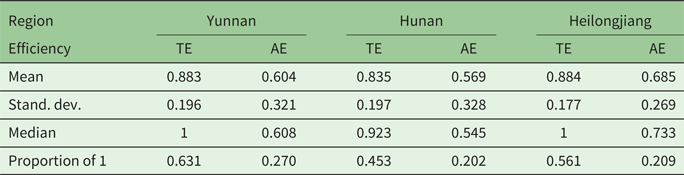
The results in table 2 show an uneven distribution of efficient households across regions. The average technical efficiency (TE) varies from 0.835 in Hunan, to 0.883 in Yunnan, and to 0.884 in Heilongjiang. Thus, households in Hunan on average produce less optimally as they tend to exhibit lower levels of technical efficiency. Yunnan and Heilongjiang have higher average TE. Note that Yunnan is also the region with the smallest farm size and the largest number of crops. This indicates that diversification in crop mix on small farms may help enhance farmers' productivity (Allen and Lueck, Reference Allen and Lueck1998). Table 2 also reports the proportion of farm households that are technically efficient (with TE = 1), with percentages ranging from 45.3 per cent in Hunan, to 56.1 per cent in Heilongjiang, and to 63.1 per cent in Yunnan. The highest percentage is in Yunnan, suggesting that farmers in Yunnan are more homogeneous in terms of technical efficiency level compared to farmers in the other regions.
Table 2 shows that allocative efficiency AE tends to be lower than technical efficiency TE. This result indicates that evaluating the prospects to improve efficiency should go beyond technical efficiency and productivity: it should also consider allocative efficiency and the prospects for improving managerial decisions in their response to market prices. Table 2 also shows that the AE scores vary across provinces. The average allocative efficiency score AE ranges from 0.569 in Hunan, to 0.604 in Yunnan, and to 0.685 in Heilongjiang. These results indicate that households in Hunan exhibit lower abilities to allocate outputs efficiently in their production activities.
In addition, table 2 reports the proportion of allocatively-efficient households (with AE = 1): they go from 20.2 per cent in Hunan, to 20.9 per cent in Heilongjiang, and to 27.0 per cent in Yunnan. In a way consistent with average AE scores, these lower percentages indicate that allocative inefficiency is more prevalent than technical inefficiency. These results show that farms in Yunnan tend to be relatively more efficient: while smaller and more diversified, they have the highest proportion of perfect efficiency (with index = 1) for both TE and AE. In other words, compared to other regions, farm households in Yunnan are in general better able to make production and resource allocation decisions.
4.2 Factors affecting rural household efficiency
Why are some rural households inefficient? Both managerial abilities and economic factors can play a role. In order to identify potential sources of inefficiency, we investigate the determinants of TE and AE. Applied to household-specific estimates of efficiency, we use a control function approach to estimate equation (7). The explanatory variables in (7) include a set of socio-economic variables that can affect farm-level efficiency. As discussed in section 2, we let ${\boldsymbol{z}_{\boldsymbol{i}}} = ({{\boldsymbol{z}_{\boldsymbol{ai}}},{\boldsymbol{z}_{\boldsymbol{bi}}}} )$ where the variables ${\boldsymbol{z}_{\boldsymbol{ai}}}$
 are potentially endogenous, i.e., correlated with the error term in (7). In our case, the variables ${\boldsymbol{z}_{\boldsymbol{ai}}}$
 include remittances, land leasing-in and land renting-out. We proceed estimating equation (7) using a control function approach given in (8a, 8b).
In a first step, we estimate the reduced form equations for ${\boldsymbol{z}_{\boldsymbol{ai}}}$ in (8a). We specify equation (8a) where the vector ${\boldsymbol{w}_{\boldsymbol{i}}}$
 includes exogenous variables that affect ${\boldsymbol{z}_{\boldsymbol{ai}}}$
 . These exogenous variables are at the household level (age of the household head), the village level (distance to the nearest bank and distance to the county center) as well as the county level (county dummy variables). These variables are all exogenous as their determination is unrelated to household-level decisions.Footnote 6
As discussed in section 2, our strategy for identifying the parameters of equation (7) relies on spatial variations. The variables ‘age’ and ‘distances’, being present in both Eqs (7) and (8a), do not play a role in identifying the parameters of ${\boldsymbol{z}_{\boldsymbol{ai}}}$ in (7). But the county dummies are present in equation (8a) and not in (7). The county dummies are excluded from equation (7) because our analysis of production efficiency already controls for agro-climatic conditions: first, the efficiency analysis is done one region at a time, thus controlling for spatial changes in climatic conditions; and second, the analysis distinguishes between three types of land: paddy land, dry land and sloped land, thus controlling for heterogeneity in land quality. This motivates why the county dummies are ‘excluded’ from equation (7). But the county dummies capture spatial effects related to migration as they reflect the spatial prospects to get access to non-farm jobs. As such the county dummies belong in equation (8a); and they provide exclusion restrictions that are needed to identify the parameters of ${\boldsymbol{z}_{\boldsymbol{a}}}$
 in (7).
The first-step estimates of equation (8a) are reported in table A1 in online appendix B. As showed in table A1, for each $j \in \boldsymbol{a}$ , the reduced-form effects of ${\boldsymbol{w}_{\boldsymbol{i}}}$
 in (8a) are found to be jointly significant at the 1 per cent significance level. Importantly, at least three county dummies are statistically significant in each equation. This supports our identification strategy using the county dummies (and associated exclusion restrictions) to identify the parameters of ${\boldsymbol{z}_{\boldsymbol{ai}}}$
 in Eqs (7) or (8b).
Under identification, the control function approach applied to the Tobit estimation of (8b) provides consistent estimates of the parameters while correcting for endogeneity bias (Wooldridge, Reference Wooldridge2015). These estimates of equation (8b) are presented in table 3, with standard errors being obtained using bootstrapping.Footnote 7
Table 3. Factors affecting efficiency – Tobit regressions
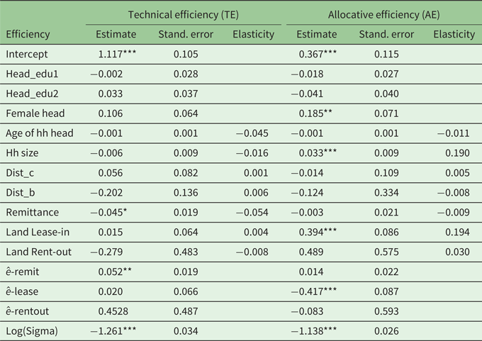
Notes: Head_edu1 is a dummy variable when the household head has at most primary school education, Head_edu2 is a dummy variable when the household head has at least high school education, Dist_c is the distance to the county center and Dist_b is distance to the nearest bank. The standard errors are bootstrapped. The stars indicate the level of significance: *** p < 0.01, ** p < 0.05, * p < 0.1. The elasticities are unconditional elasticities evaluated at sample means.
Table 3 reports that some of the predicted residuals $\hat{e}$ 's are statistically significant. This statistical significance amounts to finding evidence of endogeneity in the econometric analysis (Wooldridge, Reference Wooldridge2015). It shows that remittance is endogenous in the determination of TE and that leasing-in is endogenous in the determination of AE. This evidence indicates that unobserved factors affect both remittances and TE, as well as leasing-in and AE, implying potential endogeneity issues and motivating our use of the control function approach.
The Tobit estimates in table 3 provide useful information on the factors affecting household efficiency. Interestingly, table 3 shows that education of the household head does not have statistically significant effects on either TE or AE. A similar result applies to the ‘distance to the county center’ and ‘distance to the nearest bank’, indicating that distances to markets do not have significant impacts on TE or AE.
For TE, table 3 shows that only the remittance variable has a statistically significant impact. The negative coefficient of ‘remittance’ implies that, after controlling for endogeneity, technical efficiency TE declines when a household receives remittance from migrating household members. This is an interesting result. Note that remittances are expected to have positive effects on household welfare as they contribute to increasing household income. Our analysis shows that remittances could have some negative effects: the migration of a household member may reduce knowledge about farm household technology, implying a decrease in technical efficiency.Footnote 8 This result indicates the presence of tradeoffs between migration and human capital formation in Chinese agriculture. While the positive effect of remittances on household income could dominate, the adverse negative impact on household technical efficiency is worth noting.
Table 3 shows that neither land lease-in nor land renting-out has a significant effect on TE. Thus, we do not find strong evidence that land rental activities contribute to increasing productivity. Note that this result differs from previous literature. For example, Chari et al. (Reference Chari, Liu, Wang and Wang2017) find that leasing rights have contributed to important increases in agricultural productivity in China.
We attribute this discrepancy to two factors: (1) measurement issues (e.g., mismeasurement of productivity in the presence of unobserved heterogeneity); and (2) the neglect of allocative efficiency in Chari et al. (Reference Chari, Liu, Wang and Wang2017). Indeed, while we agree with Chari et al. (Reference Chari, Liu, Wang and Wang2017) that there are large gains from land tenure reform (as discussed below), our analysis indicates that these gains come from improving allocative efficiency (and not technical efficiency). Such an argument stresses the importance of distinguishing between technical and allocative efficiency in the economic analysis of land tenure arrangements.
Table 3 also reports the estimates of factors affecting allocative efficiency AE. It uncovers several statistically significant effects. The coefficient of ‘female head’ (0.185) is positive and significant at the 1 per cent level. Thus, while households with a female head account for less than 10 per cent of the respondents, we find that female-headed households exhibit superior allocative efficiency (compared to male-headed households). In our data, most female household heads are widows. Finding that female-headed households perform well is interesting, possibly reflecting self-selection issues (e.g., if less capable widowed females choose to marry again, leaving more capable females becoming household heads).
From table 3, larger households are found to have higher allocative efficiency, showing the presence of household size effects in managing the portfolio of household resources. The effects of remittance on allocative efficiency AE are statistically insignificant. While we found (negative) effects of remittance on TE, it seems that remittances do not play much of a role in influencing the allocative efficiency of these rural households.
The AE results in table 3 shows that the coefficient of the land lease-in variable (0.394) is positive and statistically significant at the 1 per cent level. Thus, the more the household leases-in land, the higher the allocative efficiency. The unconditional elasticity of AE with respect to ‘lease-in’ is 0.194: a 10 per cent increase in the lease-in ratio generates a 1.94 per cent increase in AE. Thus, we find that leasing land opens new opportunities for household resource management, opportunities that contribute to an improved ability to respond to market conditions and leading to significant increases in AE. Noting that higher AE implies higher household income, we obtain our main finding: leasing land contributes to large improvements in AE and in household income in rural China.Footnote 9
This result indicates that severe land scarcity imposes constraints on the ability of Chinese household managers to be allocatively efficient, and that leasing land helps lessen these constraints. Such linkages reflect the presence of significant interactions between land scarcity and allocative inefficiency. Land being a necessary input in agriculture, our results suggest that severe land scarcity reduces the ability of human capital to contribute to improved farm management and high AE. Again, such arguments stress the importance of distinguishing between technical and allocative efficiency in the analysis of land tenure issues.
Interestingly, table 3 shows that land renting-out has also a positive impact on AE, but this effect is not statistically significant. This result indicates that the benefits of rental land reform are asymmetric: most of the rural benefits accrue from leasing-in and not from renting-out. This finding may reflect the fact that land leasing-in activities are much more common than renting-out in our sample (see table 1). In other words, the linkages between allocative efficiency and land scarcity discussed above seem to be more specific to land leasing-in (and not land renting-out). This points to heterogeneity in the benefits generated by land tenure arrangements.
Finally, to check for the robustness of the Tobit results presented in table 3, we also estimated equation (8b) using two alternative econometric methods. The first method involves specifying and estimating a nonlinear parametric form for the mean of E in (7) (Papke and Wooldridge, Reference Papke and Wooldridge1996). Given that E has an upper bound of 1, we chose $mean(E )= 1 - \textrm{exp}({ - Z\; \gamma } )$ , where $mean(E )$
 is the expected value of the efficiency index E, $Z = ({{Z_1},\; {Z_2}, \ldots } )$
 are explanatory variables and $\gamma = ({{\gamma_1},\; {\gamma_2}, \ldots } )^{\prime}$
 is the vector of corresponding parameters (with ${\gamma _i} > 0\; ( < 0)$
 when ${Z_i}$
 has a positive (negative) effect on $E$
 ). The corresponding nonlinear least squares estimates are presented in table A2 in online appendix B.
The second method relies on the censored regression estimation of the median of E (Powell, Reference Powell1986). The estimation of the median has two advantages over the other two methods: (1) it is not sensitive to distributional assumptions; and (2) it is not sensitive to outliers. The censored regression estimations of the median of E are presented in table A2 in online appendix B. The statistical significance of the estimates reported in table A2 and their qualitative implications are broadly consistent with the Tobit results discussed above. This indicates that the econometric estimates reported in table 3 and their economic implications are robust.
5. Conclusion
Over the past twenty years, land tenure security in China has been gradually enhanced with longer contracts, less frequent reallocation and more rental opportunities among farmers. But questions remain about the real impacts of land rental markets on rural household efficiency.
Based on a 2009 cross-section data set of farm households in Heilongjiang, Hunan and Yunnan provinces, we estimate technical and allocative efficiencies at the household level. We show that participation in the land rental market does not affect technical efficiency but has large positive effects on allocative efficiency. Since higher allocative efficiency improves household income, our analysis shows that land rental transfers contribute to significant increases in household income in rural China. As such, land reforms have contributed to significant economic growth among rural households in China. We find that the main benefits of land reform have come from land-leasing and from improvements in allocative efficiency. Our analysis indicates that severe land scarcity imposes constraints on the ability of Chinese household managers to be allocatively efficient and that leasing land help reduce these constraints.
Our paper points to a need for further research. First, the linkages between farm household efficiency and migration need to be better understood. The effects of migration on rural welfare can be positive (e.g., from remittances) as well as negative (due to loss of labor and human capital in farm households). We find evidence of negative effects of migrations on household technical efficiency. Additional studies are needed to explore these linkages.
Second, our analysis suggests that allowing for land right transfers contributes to a greater ability of human capital to support allocative efficiency. This suggests that interactions between human capital and resource management are relevant in the analysis of land tenure issues. Further research is needed on this topic. Third, our approach was static and based on cross-section data. It would be useful to study the dynamics of efficiency adjustments associated with land tenure reform. Finally, our analysis focused exclusively on China. Our approach could be extended to examine land tenure issues in the broader context of the process of economic development around the world.
Supplementary material
The supplementary material for this article can be found at https://doi.org/10.1017/S1355770X20000583
Acknowledgements
The authors would like to thank Professor Xinqiao Ping for generously giving us the permission to use the 2009 Rural Finance Survey data, which was sponsored by the Citi Foundation.


 Open access