


1. INTRODUCTION
“One knows from previous travels how long a journey can take. When the speed varies, and how to predict it. [This is] based on experience mainly. Can you digitise this information?” (Words of a very experienced captain.) Autonomous systems are becoming more and more common in maritime e-Navigation. In other words, machines are slowly replacing people. The juxtaposition between the person and the machine often boils down into considering human factors (Chauvin, Reference Chauvin2011), or failures in human-machine communication (Lützhöft and Dekker, Reference Lützhöft and Dekker2002), which both have negative connotations towards human defects. However, in order for a ship's navigation system to reach the level of autonomy equivalent to a human navigator the machine needs to be taught by a human. The subsequent question is, are all the relevant factors that the navigators use for route planning yet digitised?
1.1. Literature review
Although literature and tools which optimise open water routes with respect to general weather can be found in abundance, the number of studies on e-Navigation for ice-covered seas is somewhat limited. Recent examples include Montewka et al. (Reference Montewka, Goerlandt, Lensu, Kuuliala and Guinness2018a), Krata and Szlapczynska (Reference Krata and Szlapczynska2018), Montewka et al. (Reference Montewka, Guinness, Kuuliala, Goerlandt, Kujala and Lensu2018b) and Li et al. (Reference Li, Goerlandt, Kujala, Lehtiranta and Lensu2018). The two most essential objectives that the majority of ice routing tools incorporate are travel efficiency (for example, time) and ship safety. These are attained with the use of various techniques that can be characterised as follows: (1) engineering-based models, (2) techniques driven by measured data, and (3) techniques based on expert models.
The engineering-based models focus on the physics of the ice-breaking process, that occurs when a ship travels through an ice field. The forces that arise in the course of ship-ice interactions are determined and the resulting added resistance against the steaming force is calculated. This approach is quite common in studies related to trafficability assessment and ice routing (Valkonen and Riska, Reference Valkonen and Riska2014; Schütz, Reference Schütz2014), despite its original purpose, which relates to ship design. Therein, the effect of ice on ship's hull and attainable speed are determined in order to provide design recommendations (Riska, Reference Riska1987; Lindqvist, Reference Lindqvist1989). Nevertheless, these models and the detailed information they provide are adopted within routing frameworks, where the forces along the hull are then considered in the time domain and in terms of what speed the ship can attain in anticipated and simplified ice conditions. In the course of its relatively long history, this approach to estimate ship performance has been validated with several field experiments and model scale tests, see for example Frederking (Reference Frederking2003), Piehl et al. (Reference Piehl, Milakovic and Ehlers2017) and Riska (Reference Riska1997). Furthermore, some of the routing tools that adopt this type of approach have been validated against historical traffic data that contains recorded trajectories of ships similar to the one used in this study, such as Kotovirta et al. (Reference Kotovirta, Jalonen, Axell, Riska and Berglund2009) and Guinness et al. (Reference Guinness, Saarimäki, Ruotsalainen, Kuusniemi, Goerlandt, Montewka, Berglund and Kotovirta2014). However, as the validation of ice routing tools is difficult, the development of several tools (Choi et al., Reference Choi, Chung, Yamaguchi and De Silva2013; Reference Choi, Chung, Yamaguchi and Nagakawa2015; Nam et al., Reference Nam, Park, Lee, Kwon, Choi and Seo2013; Schütz, Reference Schütz2014) has been progressing ahead of a thorough validation of these tools.
Data-driven models take advantage of the data from full-scale campaigns for a given ship navigating in ice. The ship speed and ice conditions are recorded and the relationship between these have been established (Montewka et al., Reference Montewka, Goerlandt, Kujala and Lensu2015; Haas et al., Reference Haas, Rupp and Uuskallio1999; Li et al., Reference Li, Montewka, Goerlandt and Kujala2017). These models are accurate for a specific ship within the range of recorded ice conditions, that is, within those various ice formations that are encountered. However, not all conditions can be accurately recorded and their effect on ship speed properly established, for example, ice compression, the presence of ice channels or that of ice breakers. Such models are suited for estimating the ship speed and whether the ship may get beset in ice. Due to their empirical origin, ship performance models are often cross-validated against recorded test data, see for example Kaleschke et al. (Reference Kaleschke, Tian-Kunze, Maaß, Beitsch, Wernecke, Miernecki, Müller, Fock, Gierisch, Heinke Schlünzen, Pohlmann, Dobrynin, Hendricks, Asseng, Gerdes, Jochmann, Reimer, Holfort, Melsheimer, Heygster, Spreen, Gerland, King, Skou, Søbjaerg, Haas, Richter and Casal2016) and Reimer (Reference Reimer2015).
Models based on experts’ judgment attempt to describe the joint effect of numerous ice features and operational conditions on a ship's safety. The focus is on estimating the trafficability of an area, prior to setting sail. Trafficability is defined as a property of the area to ensure safe passage for a ship. In some cases the speed of the ship is also considered, although this is secondary as an objective. The overall consideration encompasses ice conditions, such as the presence and formation of first- and multi-year ice, and the operational conditions meaning the presence of icebreakers. Since these models are founded on experts’ knowledge per se, encompassing the mechanics of the ice as well as ice services present in the area, they can be considered thoroughly validated for the purpose of safe route selection, see for example Stoddard et al. (Reference Stoddard, Etienne, Fournier, Pelot and Beveridge2016) and Liu et al. (Reference Liu, Sattar and Li2016).
1.2. Gap identification
The validation of e-Navigation tools is important, so that they can be trusted. Mainly, there are two questions: whether the Ship Performance Model (SPM) is valid, and whether the Ice Routing Tool (IRT) is valid. Using this differentiation between SPM and IRT, we list a review of some related work in ice-aware ship route optimisation in Table 1. Specifically, the SPM describes the extent that the model can correctly predict a ship's speed in given local circumstances, and IRT indicates the appropriateness of the method in given operational settings and maritime traffic system requirements. There are several levels of conformity for an ice routing tool, for example:
(1) The SPM is validated for a given range of ice conditions, and the IRT is validated;
(2) The SPM is not present, although the IRT is validated;
(3) The SPM is validated for a given range of ice conditions, but the IRT is not validated;
(4) The SPM is not present, and the IRT is not validated;
(5) Neither SPM nor IRT are validated.
Table 1. The summary of ice routing tools available in the literature.

The literature analysis demonstrates that if an IRT adopts a SPM, the SPM is usually validated. It is noteworthy, however, that among the 11 reviewed ice routing tools there was only one that was validated with expert knowledge, Liu et al. (Reference Liu, Sattar and Li2016). This particular tool is designed to deliver the big picture of areas that are safe for ice navigation, and it does not include detailed speed information. Two other tools were passively validated with the use of historical traffic data, Kotovirta et al. (Reference Kotovirta, Jalonen, Axell, Riska and Berglund2009) and Guinness et al. (Reference Guinness, Saarimäki, Ruotsalainen, Kuusniemi, Goerlandt, Montewka, Berglund and Kotovirta2014). The progress on the remaining eight ice routing tools has been published with their full validation still lagging behind. In the authors’ opinion, to perform a full validation of an ice routing tool, its results should be checked not only passively against historical data but also actively against decisions done by appropriate experts, to make sure that all the global and local requirements of a transportation system where a ship is operating within are met (Drost, Reference Drost2011).
1.3. Objectives of the paper
Based on the above, the goal of this paper is as follows. We introduce results obtained from experienced sea captains that are intended to be comparable with those obtained from computational e-Navigation tools, including our own ICEPATHFINDER (Lehtola et al., Reference Lehtola, Montewka, Goerlandt, Guinness and Lensu2019). These seafarers were interviewed systematically by the authors in the course of a dedicated workshop to obtain elaborated reasoning behind their route selection, and to let us decipher what knowledge yet needs to be digitised in order to advance on the ladder of system autonomy. For the results, we are able to present qualitative comparisons of the selection justification, especially when human-planned routes differ from the computed one. The range of experience for the selected ice navigators varies, ranging from experienced ice advisers to commercial ship seafarers, although all have experience of operating in the Baltic Sea. Additionally, we kept track of deck ratings while studying the different beneficial impacts that our e-Navigation tool ICEPATHFINDER had in helping the seafarers to estimate the ship performance in ice conditions. Note the somewhat analogous study on the benefits of an Electronic Chart Display and Information System (ECDIS) conducted at sea (Gonin and Dowd, Reference Gonin and Dowd1994).
The hypotheses we seek to test are that (1) the newly proposed speed and time maps for ships navigating in ice-covered waters assist the seafarers, especially those with less experience, (2) we obtain the knowledge of those aspects that our computational algorithm does not yet capture, and (3) the justifications for a certain route can be the same regardless of whether the route is planned by a man or a machine. Finally, (4) our objective is also to provide a set of validation way-points so that the future works in ship routing could benefit from ours by using these way-points as a test bench. To our best knowledge, this is the first study of its kind.
The paper is organised as follows: Section 2 introduces methods and data used, in Section 3 the obtained results are shown and are further discussed in Section 4, and Section 5 concludes the paper.
2. METHODS AND DATA
Our aim was to use experts’ knowledge to provide a validation for a specific ice routing tool, but also to study how such e-Navigation tools can be validated in general. The experts’ knowledge was elicited, for the purposes of this paper, in a route planning workshop for seafarers experienced in ice navigation that was held at Novia - University of Applied Sciences - premises in Turku on 15 December 2017, see Figure 1.

Figure 1. The workshop and the tools provided for the seafarers.
2.1. The workshop
There were eight workshop attendees as follows: two very experiencedFootnote 1 ice breaker captains that operate mainly in the Baltic Sea, working previously with large ice going ships in the Baltic and Arctic seas; two very experienced sea captains working on large ice going tankers, that operate mainly within the Baltic Sea; one experienced captain with an ice pilot background and another alternating between the roles of captain and chief officer, both working on medium-size ice going cargo vessels regularly sailing on the Baltic Sea; and – for a stark contrast – two deck ratings with limited sea and no ice navigation experience. Lower deck ratings were included in the workshop to obtain a reference point to what inexperienced seafarers who are foreign to arctic navigation would do. In order to remove individual bias, these two persons were working together to draft a single plan. Our hypothesis was they would do nothing but follow the suggestions provided by the machine – and this was confirmed during the workshop.
The participants were divided into two equally experienced groups, A and B, see Table 2. We planned the work flow so that both groups A and B got to test the augmented information tools, that is the speed map and the time map. Therefore, group A was the control group for two route cases, and the test group for two route cases, see Table 2 for elaboration. During the workshop, all attendees were working in the same room, but instructions were given, and monitored, that talking about the exercise was allowed only after everybody had completed the task at hand. This prevented the contamination of results between the control group and the test group with augmented information. Also, for the same reason no computed results or Automatic Identification System (AIS) routes were shown to or discussed with the seafarers prior to or during the workshop.
Table 2. The organisation of work for the two groups and four exercise cases in the workshop. C: control group. T: test group with augmented information, that is, speed and time maps. Lunch was served between Sessions I and II.

Prior to a route planning, the following items were given to each seafarer: (1) a mission briefing with the approximate start and end coordinates as in Table 3, (2) the ice map for that specific departure time provided by the Finnish Meteorological Institute (FMI) (e.g. right image in Figure 1 or Figure 4a), and (3) regular navigation charts with pencils and compasses.
Table 3. The four computed routes with latitude and longitude coordinates.

In addition, all participants were offered (4) Synthetic Aperture Radar (SAR) satellite images visualised on tablets, providing extra information about ice conditions. To our surprise though, none of the participants used these images. One ice breaker captain said:
“SAR images are very hard to interpret, even for experts. Even skillful people may err [that is, misjudging the pattern seen at the image] and this may have bad and serious results.”
Both ice breaker captains suggested the use of ice maps over the SAR sea-ice images:
“An ice map contains more information than the satellite images.”
Wind conditions were taken to be nominal, except for the Kemi-Hamburg route. For that route, we provided to all the workshop participants (5) a wind prediction map representing the historical wind conditions for the day of travel.
The control group members had at their disposal the tools (numbers 1–5). The test group was given on top of these (6) a speed map and (7) a time map, both as in Lehtola et al. (Reference Lehtola, Montewka, Goerlandt, Guinness and Lensu2019). The information content of the speed and time maps are briefed below, and samples of these are shown in the Results section.
2.2. Data
Both computer and human originated route data is used for this paper. Digital coordinates and dates for the chosen routes from and to the named ports are documented in Table 3, and the routes calculated using these are visualised with different colours in Figure 2. The routes begin and end at the positions where a ship with 10 m draught can navigate freely, that is, where choices can be made, outside any official ship waterway that leads to the named port. For details, see the official electronic sea maps provided by the Finnish Transport Agency (2017). The human-originated route data is from the workshop and is illustrated later in the Results section, see Figure 3. Overall, the four routes were chosen so that they would well represent the typically used routing paths and areas. The selection of routes was conducted by us before the workshop while consulting an experienced ice going sea captain who did not participate in the workshop.

Figure 2. The planning area of the workshop is the Baltic Sea. Ports and routes listed in Table 3 are shown with red circles and lines of different colors for visualisation purposes. ÅA and SA denote the Åland archipelago (forming the Archipelago Sea) and Stockholm archipelago.

Figure 3. Winter-time TSS areas are visible, when all the planned routes are plotted at once. The route lines are not entirely on top of each other as the workshop participants-instead of providing us numerical way points-commonly used a side note saying that the exact TSS route is followed. Note that in addition to the shown three TSS areas, all the ports also have regulated approaches.
Speed maps, time maps, and computed optimisations for routes listed in Table 3 are obtained from our computational routing tool (Lehtola et al., Reference Lehtola, Montewka, Goerlandt, Guinness and Lensu2019). The tool is open sourceFootnote 2. For the reader it suffices to know that the method combines ice data with data on a specific ship's performance in ice and bathymetry information with the draught of that ship to compute an optimal navigable route with A* algorithm. To this end, ice data (Helsinki Multi-category sea Ice model, HELMI) is obtained from the Finnish Meteorological Institute so that each 6 h time step is represented by a 1 NM × 1 NM grid resolution. The time stamps in Table 3 are from February and March of 2011, representing challenging conditions (see for example the ice map in Figure 6a). The ship performance model for a certain ship with the ice class ‘IA super’ is obtained from Kuuliala et al. (Reference Kuuliala, Kujala, Suominen and Montewka2017). Bathymetry information is obtained from GEBCOFootnote 3.
3. RESULTS
All human-originated route data is shown in Figure 3. The workshop participants were instructed to extend their planning down to 57° latitude, but since open water started at around 59° latitude, most participants extended their planning only so far. They complemented their planning by writing side notes that the Traffic Separation Scheme (TSS) is followed from 59° southward. Hence, the TSS plays an important role for the captains and it is equally important to outline it here. Also, we shall give an outline on ice breaker operations, similarly based on the multiple comments we obtained during the workshop. After these outlines, we shall discuss each route case separately to bring out the justifications behind the drafted plans. During this, we will try to focus on how the captains see things. To help the reader, the following route specific plots are shown so that the control group results are always in black, although (as we explained in Section 2) the control group changes according to Table 2.
3.1. Traffic Separation Scheme
In summertime, all maritime traffic in the Baltic Sea is regulated by the Traffic Separation Scheme (TSS), a ship routing system that has been adopted by the International Maritime Organization (IMO). One very experienced ice breaker captain describes (anonymised quotes from the captains are part of our results):
“The TSS is not in use during heavy ice, will be announced in the Notices to the Mariners and there will be announcement through Navtex. It will be given well in advance and valid for a quite some time, that is, for weeks.”
Officially, the decision to cease the use of TSS is made by the Transport Agency of the country responsible for a given sea area. In wintertime, the TSS is not enforced with the exception of certain narrow waterwaysFootnote 4. These narrow waterways include entrances to the ports, but also importantly the Kvarken passage and the passage between Stockholm and Åland archipelagos. The seafarers followed these regulations very strictly during the workshop. Strict instructions by us to provide numerical waypoints, however, were not followed in most cases. Instead, when the participants entered TSS areas they commonly used written side notes saying: “the TSS route is followed”. This was similar for the harbour entries, which describes how elementary these two are to the planning. (The harbour entries are also excluded from the computed routes, see Section 2.2.)
The TSS areas with all the planned routes are shown in Figure 3. For a vessel with up to 10 m draught, there are two passes from Gulf of Finland to Gulf of Bothnia. One is between Stockholm and Åland, and the other is through the Åland archipelago. Archipelago routes are typically avoided, as a very experienced captain describes:
“Sometimes you need to use a pilot and change [the pilot] in between the archipelago route, which could be more expensive than to go around the archipelago.”
3.2. Ice breaker operations
We consolidated the following key points from the interviews. (1) The Ice Breakers (IBs) give advice, not commands, on where to navigate. This advice is in the form of Waypoints (WPs) that form a DIRWAY, that is, a directed way. (2) The IBs choose when and who they will assist. Their assistance is focused on DIRWAYs. Some words of a very experienced captain:
“Some follow the ice breaker route to the dot, due to fear that they will not get help if they deviate even a little bit. But if you are an experienced ice navigator, you can deviate from the route a little bit because you can see it is easier “over there”. Following for example another track close by. WPs by ice breakers are to control the traffic and be efficient to help … the vessels. The route is there for a reason, but it is still advice. IBs do not tell where to go. Ice breakers are close to “this route” and if you get stuck, you will get help. If you navigate by yourself, you will get assistance but it will take longer. For example, if you are 50 miles away and alone, and all other traffic is somewhere else, it will take time before the ice breaker can come and help. \noindent It is typical that the vessels are asking permission to deviate from the route. During the night it is more difficult to find the route. Ice breakers have good search lights, better than commercial vessels. It is easier to get stuck in the night when you can not see properly.”
The ice breakers are, however, not the only means of moving ahead in ice. (3) The ships can assist each other, or follow one another. Another very experienced captain states:
“It is mainly the ice breakers who help those who get stuck, but sometimes vessels from the same company can help each other, that is if one gets stuck, the other one helps them to get loose from the ice.” \noindent “Some smaller vessels like to follow bigger vessels, but bigger vessels find it a bit risky.”
One tanker captain put it particularly bluntly:
“We do not like it when the smaller vessels follow us.”
This is because the leading ship fears the risk of ship to ship collision that might be caused by an ice-originated sudden decline in speed. (4) Even though ice breakers collaborate to some extent, each country has its own ice breakers, which operate in their respective domestic waters.
“In principle, if a vessel goes into the Estonian waters, Finnish ice breakers will not help.”
(5) WPs are more commonly given to enter and leave ports than to navigate in the open sea, at least in the Gulf of Finland. An ice breaker captain elaborates:
“Ice breakers usually do not give any way points in the Gulf of Finland. Maybe just outside the ports, but not really out on the open sea. Maybe [they give] just a point to collect the vessels, so that they all come to the same position. If we know a certain area which is very difficult, we give a point for the vessels coming to Finnish ports. [There is] so much traffic in the Gulf of Finland, strong vessels and much less ice [than in the Gulf of Bothnia]. When a foreign vessel comes, they are not experienced with ice so they contact an agent who contacts the ice breakers. Then the ice breakers will provide some way points, maybe 2-3 and some recommendations. GOFREP give also some ice advice/waypoints that ice breakers have given, when the situation is really bad. Very seldom there are waypoints in the Gulf of Finland, because there really is no [hard] ice.”
Here, the GOFREP refers to the Gulf Of Finland Reporting System. It is a mandatory ship reporting system under SOLAS regulation V/11, including Tallin (Estonia), Helsinki (Finland), and St. Petersburg (Russian Federation) Traffic.
3.3. Hamina-Rauma
The Hamina-Rauma ice map and routing plans are shown in Figure 4(a) and 4(b), respectively. In the Archipelago Sea, the ice does not move as it is fastened in between the islands (so-called fast ice). Notably, only one workshop participant decided to go through the Archipelago Sea (see Figure 5), and not through the passage close to the Stockholm archipelago (Sea of Åland). He had augmented tools. Additionally, it turned out that he originated from near that archipelago and used to be an ice pilot, details that might have affected the participant's decision, since the ice routing tool does not take a stance on whether it is advantageous navigate in fast ice or not.
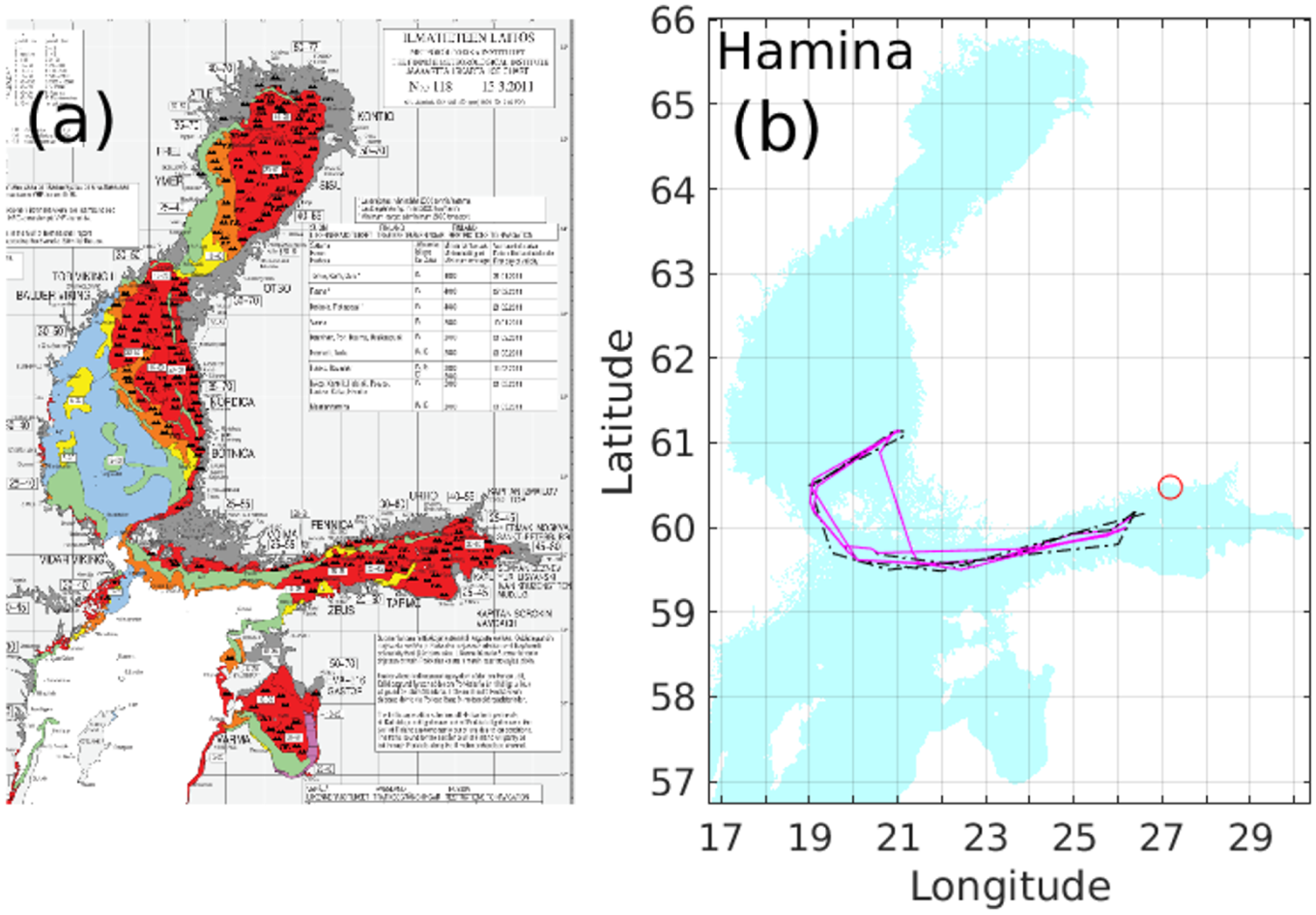
Figure 4. (a) Ice map reproduced with the permission of FMI. (b) Hamina-Rauma routes planned in the workshop, one from each participant. The augmented and control group results are shown in solid magenta and dotted black lines, respectively.

Figure 5. Augmented information as given to the workshop participants, a close-up view on the Hamina-Rauma route. (a) Speed map displaying the speed of the given ship in knots. (b) Time map indicating an estimated time of arrival (ETA, in hours), with the optimal routing area shown in cyan. The other map colours represent costs in time if a deviation is made from the computed optimal route.
There was some deviation in the planning also in the Gulf of Finland e.g. in front of Kotka, Hamina, and Helsinki. One experienced captain – using augmented knowledge – navigated closer to the northern coast of Gulf of Finland than the control group:
“The way looks easier closer to the coast.”
The captain was referring to the large ice channel visible in the ice map and the speed map. However, other captains including the control group followed a conservative path away from the coast. Navigating just outside the Gulf of Finland archipelago is risky because if there is a strong southerly wind, it can push all the ice towards the archipelago. Any ship navigating between the previously formed but separated ice ridges is likely to get beset in ice when the gap closes, and while being beset, risks grounding. This risk of turning wind was spoken out by a more experienced participant:
“One option would be to go along the [outline of] Finnish coast archipelago, but it is not worth it since the ice gets packed there [by the wind]. Better stay away from the ridged ice.”
The optimal (cyan) area, that is, the ice channel, shown in the time map, see Figure 5(b), thus appeared to have negligible guiding effect per se.
3.4. Kotka-Gdansk
From Kotka (Finland), see Figure 6, all participants would follow a similar route towards Gdansk (Poland): the summertime TSS. There were two minor exceptions. One participant using augmented information, and one without, would navigate closer to the Estonian coast than the others to avoid ice.
“There is easier ice on the Estonian side. [My] decision is based on the ice chart. This happens every winter [that] the vessels are using either the Finnish side or the Estonian side depending on the prevailing winds. [One] can be close to the coast, but you have to be careful. We also make a risk assessment of the route plan before it is accepted. Risk areas are discussed together. [We keep] safety distances and put alarms into ECDIS. It is important to put the alarms into the system, because they keep you awake about the risks.

Figure 6. (a) Ice map reproduced with the permission of FMI. (b) Kotka-Gdansk routes planned in the workshop, one from each participant. The augmented and control group results are shown in solid magenta and dotted black lines, respectively.
3.5. Kemi-Hamburg
A wind map (not shown) was handed out to each participant as additional material specifically for the Kemi-Hamburg route, shown in Figure 7. The wind map did not affect the planning north of Kvarken, the wind being negligible thereabouts. The small routing differences in the bay of Bothnia are because the participants had to make their own assumption of the location of the ice breaker DIRWAY.
“[Steam] with the help of an ice breaker from Kemi to 64·48° latitude and 22° longitude.”
In TSS regulated areas, Kvarken and between Åland and Stockholm, the routes expectedly converge. In between, however, the different level of information that we provided to the two groups made a significant difference, and the control group diverged westwards towards the Swedish coast from a geometrically straight path that was followed by the group with augmented information. See Figure 7b. The participants in the control group explained their choices:
“Steam by the Swedish side because of the ice map, and the wind map. The wind pushes the ice towards the Finnish coast. In addition, the sea is deeper on the Swedish side and the ice cover is generally lighter.”
The test group on the other hand had the possibility to see from the speed and time map that the ice cover was so lightFootnote 5 that it had little effect on the journey. One very experienced captain commented on the lack of information from the augmented tools, while making a choice (that surprised us) to steam close to the Swedish coast:
“It would be useful to get the ice chart on the ECDIS. Poor internet connection sometimes in the vessel [does not allow us] to study the ice chart. It would be easier for route planning if all information would be layers on ECDIS. Canadians have different layers on their ice charts.”
It is our interpretation that the captain would have wanted to see the ‘raw’ ice data while the conclusion about the best route had already been made by the computational method, and put out into the form of speed and time maps. Since the raw data was not available, the captain was obliged to distrust the routing tool and choose a safer route.

Figure 7. (a) Ice map reproduced with the permission of FMI. (b) Kemi-Hamburg routes planned in the workshop, one from each participant. The augmented and control group results are shown in solid magenta and dotted black lines, respectively.
Note that the augmented tools for the Kemi-Hamburg route are shown in Figure 8 with additional plots that were not available to the workshop participants. The black computed optimal route, a blue AIS route from a ship with similar ice performance that traveled the route during the given day, and the routes planned by the participants are shown. When leaving from Kemi, the computed optimal route directly aims for the open water, while workshop participants were allowed to make their own assumptions on where the DIRWAY (shown by the blue AIS plot) could have been. South of Kvarken, the computed optimal route and the routes planned with augmented tools agree, while the traditionally planned routes are more west-bound. The speed and time maps clearly show that the thick-looking ice cover in Figure 7(a) in fact is quite easily traversable for the given ship.

Figure 8. Kemi-Hamburg route. (a) Speed map displaying the speed of the given ship in knots. (b) Time map displaying the computed optimal route with solid black line. The map is coloured with costs in time, if a deviation is made from the computed route. The AIS route of a similar type ship that had traveled that day is in blue, and the workshop planned routes in dotted black and magenta lines as previously.
3.6. Oulu-London
For the Oulu-London route, the upper part of the Gulf of Bothnia contained thick ice and ridges, see Figure 9.
“Probably need ice breaker assistance from Oulu to easier ice. There are Finnish ice breakers. Very normal that one in the Kemi area and two others more south. Very cold and westerly winds, so a lot of ice on the Finnish coast. A lot of ridges.”
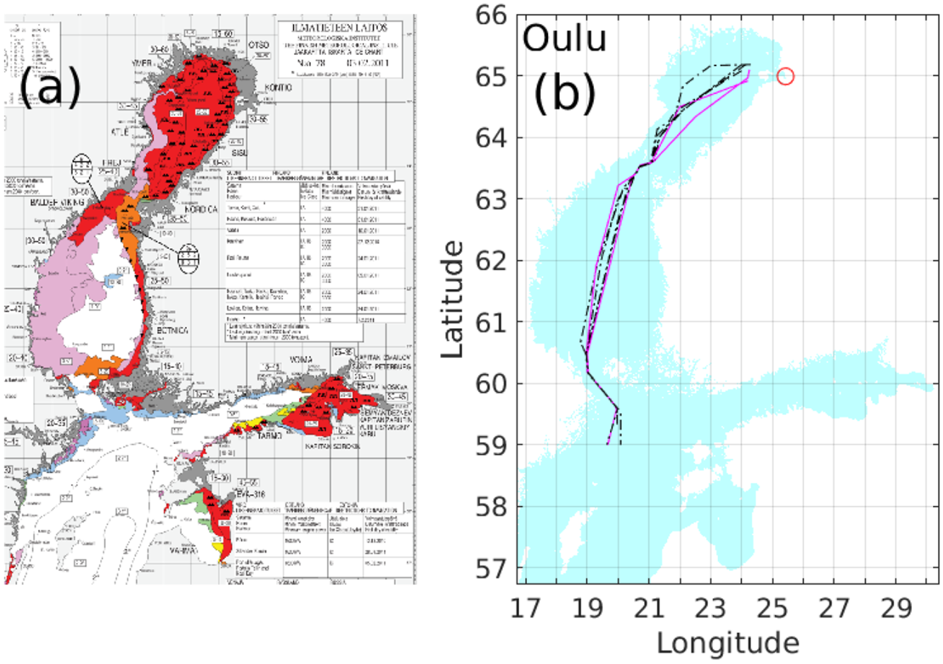
Figure 9. (a) Ice map reproduced with the permission of FMI. (b) Oulu-London routes planned in the workshop, one from each participant. The augmented and control group results are shown in solid magenta and dotted black lines, respectively.
Participants with augmented information would take a more southern route from Oulu than the control group. They assumed that this is where the DIRWAY is, as we did not give a specific answer to their question about it.
“The time map is showing clearly where one can steam.” \noindent “Having the speed and the time map in addition to the ice maps gives a sense of security. One can found one's decision on more sources of information than one. It makes decision making easier.”
Between Kvarken and Stockholm TSSs, participants could be divided into two categories. Some preferred a straight route, while some took a west-swinging detour due to the ice situation. The interesting thing here is that the most experienced captains preferred the straight route,
“The rest is easy ice and open water.”
while the more inexperienced participants avoided the thin ice somewhat unnecessarily.
“[Go] via the Swedish side, so that the ship does not get beset in ice.”
3.7. Missing data
From the interviews done at the workshop, we gathered notes on what information the seafarers would use if they could, in specific situations. In other words, we attempt to list the information (or data) that are missing from the current e-Navigation routing tools. The most common thing was related to ice breaker operations:
“I'd need to know the IB or VTS [Vessel Traffic Service] WPs for entering and leaving the ports.”
They all said the following critical “but-sentence” when given only the ice map as knowledge, and asked for a route plan:
“But I would ask for the ice breaker DIRWAYs, and look for the open ice channels from AIS data.”
What the mariners would look for from AIS data is:
“I'd follow a big and strong ship.” \noindent “Especially in [Åland] archipelago I'd rather follow someone, since the ice channel can freeze shut in a few hours, if the temperature is very low.”
One ice breaker captain summed his findings as:
“In contrast to reality, this workshop is missing the DIRWAYs, the ice history, the weather predictions, and the knowledge on where other ships are operating.”
However, interestingly, another ice breaker captain strongly disagreed on whether the ice history actually is relevant information.
“I totally disagree [with him] on using historic ice maps. They are useless. Only the forecast information is worthwhile.”
3.8. Feedback on e-Navigation routing tools
We received feedback on the speed and time maps that they would be useful in helping the planning of the route schedules.
“All ETA estimation tools are welcomed by ship owners, harbours, etc.”
Specific reasons for this were elaborated by one participant:
“The schedules are planned the same – in summer and in winter. If time is lost due to winter conditions, faster speed is used to catch up the schedule – or for example, Kiel canal [shortcut]. Nowadays schedules are quite tight, so it might be that shipping companies forget that there can be severe ice conditions and book the ships with a tight schedule.”
This issue probably is related to the experience level of the scheduler. As an ice-breaker captain pointed out:
“Experience in planning the ship routes is important especially in the winter, because they need to optimise (not too tight and not too loosely) the scheduling of the ship.”
In addition, our ICEPATHFINDER implementation (Lehtola et al., Reference Lehtola, Montewka, Goerlandt, Guinness and Lensu2019) received positive feedback when the accuracy of the ice maps was discussed, since ICEPATHFINDER handles level ice and ridged ice separately. Specifically, the harshness of the ice conditions is directly visible in the speed map. This is in contrast to the ice maps, where for example all ridged areas are shown as red even though the severity of the ice conditions varies within the ridges. A captain noted:
“In the [Oulu] speed map it was obvious that within the ridged area, some part of it was with such a low concentration that IA super [ice class ship] can maneuver well therein. But then in the Northern part of it the concentration was at such level that.. yes, it is a No-Go zone.”
This captain went on to propose that the ice-covered areas could be divided into ‘go’ and ‘no-go’ zones to increase safety in ice navigation.
The workshop participants seemed to want to visually interact with the route planning tools:
“Use of speed map and time map, interesting piece of information. But all you can see is what the computer sees is the fastest route. It would be nice to have an ice chart on top of it for comparison.” \noindent “[I'd] Study the ice chart and check from ECDIS the limits of ice and also study the ice breaker advice. Then [I'd] have discussions in the team and try to take the shortest way in the heavy ice.”
Before deciding to enter ice fields, captains typically look at the wind forecast and ice maps to estimate whether there is pressure or not.
“Pressure is the most challenging thing [in ice navigation].” \noindent “Some areas with some winds do not have any pressure at all and suddenly you have a lot of pressure.” \noindent “Compression [of the ice field] should be implemented to the tool. Compression is directional, so navigation is possible in some ways, and in some ways it is not.”
Ship sensors were suggested to be integrated to the external ice information:
“In level ice, the ship radar can see used routes within the radius of a few nautical miles.”
The predictive abilities of e-Navigation tools raised questions. In particular, whether the ice class of a ship is a good way of categorising that ship's performance.
“Previously ships had more power than their ice class minimum requirements would indicate. Now ships are planned to match the minimum performance requirements.”
From an ice-breaker captain's point of view, also damage control plans for the worst case scenarios are needed:
“The wind forecast is important, but 48 h forecast may underestimate the conditions. Typically we use less than 24 h time window to make decisions on IBs. There is a need also to plan ’damage control’ if conditions will be actually worse than what was forecasted 24 h beforehand.”
4. DISCUSSION
Automated ice navigation methods cover a mid-regime between two states. In the summer state, the open water traffic in the Baltic Sea is guided by the TSS. In an extreme winter state, ridged ice fields cover the sea areas and there is no room for self-navigation: ice breakers must be followed. The ice navigation methods are thus intended to cover the middle regime between these two states, summer and extreme winter. Hence, as we also observed in the Results, the routes planned by seafarers follow the TSS, except when the ice conditions create a reason to deviate from it. Technically, this could be described with a simple algorithm as follows: The optimal route is the shortest TSS route, corrected with the most optimal deviation given that this deviation increases travel safety and efficiency. Each planned route by the workshop participants described with a set of waypoints their version of this ‘optimum’ path. This algorithm is quite similar to the current e-Navigation methods, including ours (Lehtola et al., Reference Lehtola, Montewka, Goerlandt, Guinness and Lensu2019), which searches a geometrically optimal route given the multi-objective data.
The ice breaker waypoints support the efficient and safe traffic flow and logistics in ice covered waters. Focusing on this means that ships getting beset in ice outside the designated travel area are less prioritised due to the cost in efficiency they pose on the whole marine traffic system. Skilled ice navigators know when and how to deviate from the route in order to find the most favourable path through the ice at the same time they follow the WPs provided by the ice breakers. As one very experienced captain put it
“Skill in ice navigation is a competitive advantage.”
Finally, in order to close the gap between the present situation and full automation, at least the following should be included in the e-Navigation tools:
• Weather risk analysis of different sea areas, especially those where the weather conditions may change rapidly in comparison to the timescale of the available weather prediction. This might be done by analysing the historical ice and weather data by means of artificial intelligence.
• Reliable analysis of go and no-go areas in ice-covered waters, given the ice conditions and the ship-specific manoeuvring properties in ice. Ice status information, for example from the FMI, is of rather good quality in the Baltic Sea, but the ship-specific properties are hard to come by, for example, such as the ones determined in Kuuliala et al. (Reference Kuuliala, Kujala, Suominen and Montewka2017).
• Digital real-time AIS data analysis, for example, to scout for suitable open ice channels that lead towards the ship's destination.
• Digital real-time situational awareness from sensors to increase navigation safety. This is achievable, for example, by integrating ship radar and other data to monitor other ships and scout for suitable open ice channels.
• Communication with ice breakers could be digitised to provide DIRWAYs directly to ships’ e-Navigation systems.
• Narrow waterways could offer positioning and other digital support for safe and automated e-Navigation, also in winter conditions.
The quotes throughout the text are anonymised and are from the captains that participated. These are from the individual interviews done for each captain and joint debriefings. We did not notice disagreement or conflict in the general narrative, except for one case related to the use of historic ice maps that we have elaborated in Section 3.7. Case by case route plans were done individually, and the deviations in reasoning behind those are elaborated in the Results section.
We shall publish the waypoints recorded in the workshop to act as a benchmark for future Arctic maritime studies. Note that for this purpose the Baltic Sea offers an excellent test bed since various reference systems are available, such as a wide coverage AIS monitoring network, high resolution weather and ice models, and abundant positioning infrastructure.
5. CONCLUSION
A digital gap exists between the e-Navigation tools of today and the autonomous navigation safety systems of tomorrow. In order to study this gap, we present here the results of a workshop for seasoned captains that are particularly experienced in ice navigation.
We tested whether the augmented tools, meaning the speed map and the time map, could lead to better and safer route planning. Results obtained with respect to the control group indicate that especially those workshop participants that had less experience benefited from these tools in terms of better planning. They also experienced increased confidence. These may both be considered to be positives outcomes that facilitate decision making. On the other hand, if – by chance – there was a systematic error in the input data affecting all the information products, this sense of safety might result in severe, unwanted outcomes. Future studies on e-Navigation tools should contain probabilistic estimates on the reliability and on the predictive capability of these tools.
FINANCIAL SUPPORT
The work in this article has been carried out in the context of the BONUS STORMWINDS project. This project has received funding from BONUS (Art 185) funded jointly from the European Union's Seventh Programme for research, technological development and demonstration, and from the Academy of Finland.


 Open access