


1. Introduction
A striking feature of chaotic dissipative systems such as turbulence is the spontaneous emergence of coherent structures, which appear as well-defined and traceable objects in the obscure collection of chaotic interactions. A paramount example in turbulent flows is the presence of long-lived coherent ‘worms’ or ‘sinews’ of intense vorticity. These structures have a relevant impact on turbulence statistics (Pumir Reference Pumir1994; Toschi & Bodenschatz Reference Toschi and Bodenschatz2009), and on diverse phenomena such as cavitation or clustering (Bappy et al. Reference Bappy, Carrica, Vela-Martín, Freire and Buscaglia2020; Mathai, Lohse & Sun Reference Mathai, Lohse and Sun2020). Since they were first detected in direct numerical simulations (Siggia Reference Siggia1981; She, Jackson & Orszag Reference She, Jackson and Orszag1990) and experiments (Douady, Couder & Brachet Reference Douady, Couder and Brachet1991; Cadot, Douady & Couder Reference Cadot, Douady and Couder1995), researchers have striven to explain their origin and quantify their relevance to turbulence theory, but to date no consensus exists. Frisch (Reference Frisch1995) described this problem in terms of whether intense vortices are the ‘dog’ or the ‘tail’ of turbulence, i.e a relevant feature of turbulent flows with dynamical significance, or just the byproduct of other underlying turbulent processes, with reduced influence on the overall dynamics.
Understanding the mechanisms by which intense vorticity structures are generated and controlled is essential to assess their relevance to turbulence dynamics. Diverse physical mechanisms (Vincent & Meneguzzi Reference Vincent and Meneguzzi1994; Passot et al. Reference Passot, Politano, Sulem, Angilella and Meneguzzi1995) and simplified models (Burgers Reference Burgers1948; Pullin & Saffman Reference Pullin and Saffman1998) have been proposed to explain their origin, but none are fully consistent with the empirical evidence. On a fundamental basis, the vorticity equation points directly to the interaction with the rate-of-strain tensor, the so-called vortex stretching mechanism, as the cause for the generation of intense vorticity. Despite extensive research focused on the characterisation of vortex stretching, the causal relations that drive this mechanism are not well understood due to its nonlinear and non-local nature (Ohkitani & Kishiba Reference Ohkitani and Kishiba1995).
Two of the most intriguing aspects of intense vortices are their disparity of scales and the scaling of their circulation. They have radii of the order of Kolmogorov units, but lengths that reach up to the inertial – or even integral – scales, and their circulation scales with the root-mean-square of the velocity fluctuations and the Kolmogorov length scale (Jiménez et al. Reference Jiménez, Wray, Saffman and Rogallo1993). These observations suggest that large and small scales are involved in their dynamics, but it remains unclear which scales control their formation and evolution. There is evidence that points in the direction of a top-down mechanism controlled by large scales. Locally, the vorticity vector aligns predominantly with the intermediate eigenvector of the rate-of-strain tensor (Ashurst et al. Reference Ashurst, Kerstein, Kerr and Gibson1987). However, when the rate-of-strain tensor is filtered, vorticity predominantly aligns with the most stretching direction (Leung, Swaminathan & Davidson Reference Leung, Swaminathan and Davidson2012; Lozano-Durán, Holzner & Jiménez Reference Lozano-Durán, Holzner and Jiménez2016), suggesting that large scales are actively involved in the dynamics of the vorticity vector. On the other hand, the scale of the worms’ radii and the dominant amplification of vorticity by the rate-of-strain tensor in the dissipative scales challenge this scenario. This evidence suggests a bottom-up process in which structures of intense vorticity may first be originated by interactions within the dissipative range, and then grow or coalesce into elongated tubes that reach up to inertial or integral scales (Jiménez et al. Reference Jiménez, Wray, Saffman and Rogallo1993).
In this paper, we shed light on the dynamics of intense vorticity by means of synchronisation experiments in direct numerical simulations of isotropic turbulence. These numerical experiments disentangle the causal relations between the vorticity vector and the rate-of-strain tensor, and confirm the relevant role of large-scale dynamics in generating and controlling intense vortices. Our results discard the view that they emerge primarily from small-scale dynamics, and connect their evolution to scales at the end of the inertial range.
2. Synchronisation experiments in isotropic turbulence
2.1. Complete synchronisation in the dissipative range
The synchronisation of chaotic systems is a well-known and widely studied phenomenon with important consequences and applications in the natural sciences and engineering (Pecora & Carroll Reference Pecora and Carroll1990). See Di Leoni, Mazzino & Biferale (Reference Di Leoni, Mazzino and Biferale2020) for a recent application to turbulence. In general, two or more chaotic systems are said to be synchronised when all, or some, of their state variables evolve towards a common spatio-temporal pattern under the action of a driving force or coupling. In particular, the synchronisation is said to be complete when the driven systems evolve towards the same states regardless of their initial conditions. As first shown by Yoshida, Yamaguchi & Kaneda (Reference Yoshida, Yamaguchi and Kaneda2005), and later by Lalescu, Meneveau & Eyink (Reference Lalescu, Meneveau and Eyink2013), homogeneous turbulence is a complex phenomenon that exhibits the complete synchronisation of the dissipative scales when driven by similar large-scale dynamics.
These synchronisation experiments are conducted as follows. We consider the incompressible Navier–Stokes equations in a triply periodic cubic domain, which describe the evolution of homogeneous isotropic turbulence,
 \begin{equation} \partial_t \boldsymbol{u} + \boldsymbol{u} \boldsymbol{\cdot} \boldsymbol{\nabla} \boldsymbol{u} ={-} \boldsymbol{\nabla} p + \nu\nabla^2 \boldsymbol{u} + \boldsymbol{f}, \end{equation}
where  $\boldsymbol {u}=\{u_i\}$ is the velocity vector, $p$ is the kinematic pressure that ensures incompressibility, $\boldsymbol {\nabla } \boldsymbol {\cdot } \boldsymbol {u}=0$, $\nu$ is the kinematic viscosity and $\boldsymbol {f}$ is a solenoidal body force that sustains turbulence by acting only on the large scales of the flow. We project these equations on a truncated Fourier basis,
 \begin{equation} (\partial_t + \nu k^2) \hat{\boldsymbol{u}}(\boldsymbol{k}) = \hat{\boldsymbol{\mathcal{L}}}(\boldsymbol{k};\boldsymbol{u}) + \hat{\boldsymbol{f}}(\boldsymbol{k}), \end{equation}
where the hat denotes variables in Fourier space,  $\boldsymbol {{\mathcal {L}}}=-\boldsymbol {u} \boldsymbol {\cdot } \boldsymbol {\nabla } \boldsymbol {u} - \boldsymbol {\nabla } p$ and $\boldsymbol {k}$ is the wavenumber vector, with $k$ its magnitude.
We now consider three different systems with similar physical parameters integrated in parallel simulations: a master system,  $\boldsymbol {u}^M$, and two slave systems, $\boldsymbol {u}^A$ and $\boldsymbol {u}^B$. Hereafter, we use the superscripts to distinguish quantities in the different systems. The master system is a standard direct numerical simulation, while to the slave systems we continuously assimilate the large scales of the master system. At each time step of the simulation, we copy the data from the master to the two slave systems for modes below a prescribed wavenumber $k_a$, so that at all times
 \begin{equation} \hat{\boldsymbol{u}}^{A,B}(\boldsymbol{k}) =\hat{\boldsymbol{u}}^M(\boldsymbol{k}), \quad \text{if } k < k_a. \end{equation}
This procedure, known as data assimilation, can be described in terms of a filtering operation using a high-pass sharp Fourier filter with cutoff wavenumber  $k_a$,
 \begin{equation} \left. \begin{gathered} G(k;k_a)=0,\quad \text{if } k\le k_a, \\ G(k;k_a)=1,\quad \text{if } k> k_a, \end{gathered} \right\} \end{equation}
which decomposes the flow field into  $\hat {\boldsymbol {u}}=\hat {\boldsymbol {u}}_l + \hat {\boldsymbol {u}}_s$, where $\hat {\boldsymbol {u}}_s(\boldsymbol {k})= \hat {\boldsymbol {u}}(\boldsymbol {k})G(k;k_a)$ and $\hat {\boldsymbol {u}}_l(\boldsymbol {k}) =\hat {\boldsymbol {u}}(\boldsymbol {k})-\hat {\boldsymbol {u}}_s(\boldsymbol {k})$ are the small- and large-scale velocity fields, respectively.
The evolution equation of the slave system ‘ $A$’ (or slave system ‘ $B$’) is given by
 \begin{equation} \left. \begin{gathered} \partial_t \hat{\boldsymbol{u}}^A_l(\boldsymbol{k})=\partial_t \hat{\boldsymbol{u}}^M_l(\boldsymbol{k}),\\ (\partial_t - \nu k^2) \hat{\boldsymbol{u}}^A_s(\boldsymbol{k}) =G(k;k_a)\hat{\boldsymbol{\mathcal{L}}}(\boldsymbol{k};\boldsymbol{u}^A_l + \boldsymbol{u}^A_s), \end{gathered} \right\} \end{equation}
where the master system drives the slave system through the actions of the nonlinear interactions present in  $\boldsymbol {\mathcal {L}}$. The initial conditions of the slave systems satisfy ${\boldsymbol {u}}^A_l(\boldsymbol {k};t_0) ={\boldsymbol {u}}^B_l(\boldsymbol {k};t_0)={\boldsymbol {u}}^M_l(\boldsymbol {k};t_0)$, and ${\boldsymbol {u}}^A_s(\boldsymbol {k};t_0)$ and ${\boldsymbol {u}}^B_s(\boldsymbol {k};t_0)$ are independent small-scale velocity fields. Considering $k_a$ as a proxy for the assimilation scale, $\ell _a={\rm \pi} /k_a$, the flow at scales above $\ell _a$ in the slave systems is always similar to that in the master system due to the assimilation procedure, while the flow below $\ell _a$ evolves ‘freely’ under the Navier–Stokes equations.
When  $\ell _a<16\eta$ (thus $k_a\eta >0.2$), where $\eta =(\nu ^3/\langle \varepsilon \rangle ^4)^{1/4}$ is the Kolmogorov length scale and $\langle \varepsilon \rangle$ is the ensemble-averaged kinetic energy dissipation, the slave systems synchronise completely and $|\hat {\boldsymbol {u}}^B-\hat {\boldsymbol {u}}^A|\rightarrow 0$ when $t\rightarrow \infty$ regardless of the initial conditions in the small scales of the slave systems. Lalescu et al. (Reference Lalescu, Meneveau and Eyink2013) report total synchronisation for $k_a\eta >0.15$, but their experiments are anisotropic in the large scales and prone to bursting.
We stress the dynamical interpretation of synchronisation: at scales below  $\ell _a=16\eta$, chaos is totally constrained by viscosity, and the dynamics is driven by scales above. Synchronisation experiments provide a framework to identify the sufficient causes of the synchronised events. The evolution of scales below $16\eta$ can be fully reconstructed with the information of scales above, while the opposite is in general not true, evidencing a strong causal connection from scales above $16\eta$ to scales below.
2.2. Partial synchronisation above the dissipative range
In this work we reproduce and extend the numerical experiments of Yoshida et al. (Reference Yoshida, Yamaguchi and Kaneda2005) for assimilation scales larger than  $16\eta$, when synchronisation is only partial and the slave systems develop their own chaotic dynamics. As we will show, synchronicity is still relevant in some parts of the slave systems, pointing to the events that are caused by scales above the assimilation scale.
We consider fully developed isotropic turbulence at two different Reynolds numbers of the master system,  $Re_\lambda =u'\lambda /\nu =120$ and $195$, where $\lambda =(15\nu /\langle \varepsilon \rangle )^{1/2}u'$ is the Taylor microscale, $u'$ is the root-mean-square velocity fluctuation and $\varepsilon =\nu \sum _k k^2 \hat {\boldsymbol {u}} \hat {\boldsymbol {u}}^*$ is the instantaneous volume-averaged energy dissipation rate. The angular brackets denote the ensemble average and the asterisk indicates the complex conjugate. These Reynolds numbers are simulated on cubic grids with $N^3=256^3$ and $512^3$ points, and all simulations are run at a fixed resolution of $k_{max}\eta =2.0$, where $k_{max}=(\sqrt{2}/3)N$ is the maximum wavenumber magnitude. Further details of the code are described in Cardesa, Vela-Martín & Jiménez (Reference Cardesa, Vela-Martín and Jiménez2017).
We explore the partial synchronisation of the slave systems for  $\ell _a$ between $20\eta$ and $40\eta$. For each different assimilation scale and Reynolds number, we have run simulations for a time of approximately $20T_{{eto}}$, where $T_{{eto}}=L/u'$ is the eddy turnover time and $L=({{\rm \pi} }/{K}) \sum _k k^{-1}E(k)$ is the integral scale. Here $E(k)=2{\rm \pi} k^2\langle \hat {\boldsymbol {u}} \hat {\boldsymbol {u}}^* \rangle _k$ is the kinetic energy spectrum, $\langle \cdot \rangle _k$ denotes average over time and over wavenumber shells of radius $k$, and $K=\sum _k E(k)$. For statistical analysis, we have collected between $20$ and $100$ independent velocity fields for each case, which are enough to converge the statistics.
In these experiments the synchronisation of scales below  $\ell _a$ is incomplete, and these scales develop their own independent chaotic dynamics, which are, however, not completely decoupled from the master system. As shown in figure 1(a), the temporal signals of the dissipation above wavenumber $k_a$, i.e. $\varepsilon _s=\nu \sum _{k>k_a} k^2 \hat {\boldsymbol {u}} \hat {\boldsymbol {u}}^*$, in the slave systems are highly synchronised to the signal of the master system. The correlation coefficient between these signals in the master and slave systems is approximately $0.99$ for $\ell _a=20\eta$, and drops only to $0.91$ for $\ell _a=30\eta$ for the two Reynolds numbers considered here.

Figure 1. (a) Phase diagram of signals of the volume-averaged dissipation above  $k_a$ for the master, $\varepsilon ^M_s$, and slave, $\varepsilon ^A_s$ and $\varepsilon ^B_s$, systems. The signals cover $15T_{{eto}}$, with markers separated by $0.1T_{{eto}}$, and correspond to $\ell _a=20\eta$ and $Re_\lambda =120$. The upper dotted line marks $\varepsilon ^B_s=\varepsilon ^A_s$, and the lower $\varepsilon ^M_s=0.93\varepsilon ^A_s$. (b) Energy spectra normalised with the total energy for the master system (dashed line) and for the slave systems (lines with markers) for different assimilation scales. The solid line is proportional to $(k\eta )^{-5/3}$. (c) Premultiplied dissipation spectra normalised in Kolmogorov units for the master system (dashed line) and the slave systems (lines with markers), and premultiplied error spectra (lines without markers), for different assimilation scales. The data correspond to $Re_\lambda =195$, but are qualitatively similar for $Re_\lambda =120$. The vertical dotted in lines (b,c) mark the assimilation scales.
In figure 1(b,c), we show the energy and the dissipation spectra,  $E(k)$ and $D(k)=2\nu k^2 E(k)$, at different values of $k_a$ for the master and slave systems. The smooth transition of the energy spectra from the assimilated data to the freely evolving modes above $k_a$ indicates a strong dynamic coupling from the master to the slave system, and the good collapse of the dissipation spectra in Kolmogorov units indicates healthy small-scale dynamics. The only significant consequence of the assimilation procedure is the increment of the average dissipation in the slave systems with respect to the master system. This increment is approximately $5\,\%$ for $\ell _{a}=20\eta$ and $30\,\%$ for $\ell _{a}=40\eta$, and leads to a slight reduction of the effective $Re_\lambda$ of between $3\,\%$ and $12\,\%$. This is a consequence of the lack of a feedback mechanism from scales below $\ell _a$ to scales above, but it does not affect the structure of the small scales in the slave systems, which have similar statistics to those of the master system. For instance, the skewness and the flatness factor of the longitudinal velocity derivatives are indistinguishable between systems. We find that $F_3\approx -0.54$ and $F_4\approx 6.3$ in all systems for $Re_\lambda =195$, where $F_n=\langle (\partial _i u_i)^n\rangle /\langle (\partial _i u_i)^2\rangle ^{n/2}$ (no summation intended for repeated indices). These values are similar to those in the literature (Jiménez et al. Reference Jiménez, Wray, Saffman and Rogallo1993).
In figure 1(c), the error spectrum
 \begin{equation} R(k)=\langle \Delta \hat{\boldsymbol{u}}\Delta \hat{\boldsymbol{u}}^* \rangle_k/\langle \hat{\boldsymbol{u}} \hat{\boldsymbol{u}}^* \rangle_k, \end{equation}
where  $\Delta \boldsymbol {u} = \boldsymbol {u}^A - \boldsymbol {u}^B$, shows that the coupling between the assimilated data and the freely evolving modes of the slave systems is very local in scale, with error increasing sharply for wavenumbers larger than $k_a$. This locality and the strong correlation of the energy dissipation signals bring to mind the energy cascade process (Zhou Reference Zhou1993; Eyink & Aluie Reference Eyink and Aluie2009; Cardesa et al. Reference Cardesa, Vela-Martín, Dong and Jiménez2015). We suggest that partial synchronisation, which we analyse in the following sections, reflects the control exerted by scales above the assimilation scale into smaller scales to produce the adequate amount of inter-scale energy fluxes.
3. The structure of partial synchronisation
In this section, we characterise the structure of partial synchronisation between the slave fields in physical space, with focus on the vorticity vector,  $\boldsymbol {\omega }=\boldsymbol {\nabla } \times \boldsymbol {u}$. A very relevant aspect of these experiments is that the local degree of synchronisation is not homogeneous in space, but depends strongly on the magnitude of the vorticity vector,
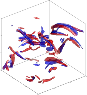
  $\varOmega =|\boldsymbol {\omega }|$. In figure 2(a,b), we show visualisations of structures of intense vorticity in the slave and master fields for $\ell _a=20\eta$ and $Re_\lambda =120$. We observe a conspicuous synchronisation of worms, which overlap or appear adjacent with the same orientation.

Figure 2. (a) Visualisation of intense vorticity structures in the slave systems ‘ $A$’ (red) and ‘ $B$’ (blue), and of structures of intense vorticity in the large scales of the master system (magenta) for $\ell _a=20\eta$. Red and blue isosurfaces (slave systems) correspond to $\varOmega ^{A,B}=3\langle \varOmega \rangle$, and magenta isosurfaces (master system) to $\varOmega ^M_l=4\langle \varOmega ^M_l \rangle$. The panel shows the full computational domain. (b) Detail of the synchronisation of intense vortices in the slave systems in a $(150\eta )^3$ subdomain. Colours as in panel (a). The data in (a,b) correspond to different flow fields from simulations at $Re_\lambda =120$. (c) Probability density function of the large-scale vorticity magnitude, $\varOmega ^A_l$ (solid markers), and the small-scale vorticity magnitude, $\varOmega ^A_s$ (empty markers), in the slave system, and the vorticity magnitude in the master system $\varOmega ^M$ (solid black line) for $Re_\lambda =120$. All quantities are normalised with $\langle \varOmega \rangle$ in each system. Dotted vertical lines mark $\varOmega /\langle \varOmega \rangle =1$ and $3$.
$3$.
These structures have a typical radius of approximately  $4\eta$, but lengths larger than the assimilation scales used in our experiments (Jiménez et al. Reference Jiménez, Wray, Saffman and Rogallo1993). As shown by the dissipation spectra in figure 1(c), the assimilated data contain a non-negligible fraction of the total dissipation ( $16\,\%$ for $\ell _a=20\eta$), and therefore of the total squared vorticity. We discard, however, the view that the assimilated data contain structures of intense vorticity. In figure 2(c), we show the probability density function (p.d.f.) of $\varOmega _{s}^A=|\boldsymbol {\omega }_{s}^A|$, $\varOmega _l^A=|\boldsymbol {\omega }_l^A|$ and $\varOmega ^M=|\boldsymbol {\omega }^M|$. Here $\hat {\boldsymbol {\omega }}_{l}= \hat {\boldsymbol {\omega }}_{}(\boldsymbol {k})(1-G(k;k_a))$ corresponds to the vorticity above scale $\ell _a$, which is assimilated from the master system, and $\hat {\boldsymbol {\omega }}_{s}= \hat {\boldsymbol {\omega }}(\boldsymbol {k})G(k;k_a)$ to the vorticity below scale $\ell _a$. Even for $\ell _a=20\eta$, the assimilated data contain only a small fraction of the vorticity magnitude above $\langle \varOmega \rangle$, and a negligible fraction of the intense vorticity above $3\langle \varOmega \rangle$, which is a threshold used to identify vorticity worms (Jiménez et al. Reference Jiménez, Wray, Saffman and Rogallo1993). On the other hand, the p.d.f.s of the total and the small-scale vorticity magnitude are very similar. Hence intense vorticity structures originate in the small scales due to interactions with the assimilated data, but are not imposed by the assimilation process.
To characterise the local synchronisation pattern of the vorticity field, we evaluate the cosine of the angle of alignment between the vorticity vectors of the two slave systems,
 \begin{equation} \cos(\boldsymbol{\omega}^A,\boldsymbol{\omega}^B)={\boldsymbol{\omega}^A\boldsymbol{\cdot}\boldsymbol{\omega}^B}/{(|\boldsymbol{\omega}^A||\boldsymbol{\omega}^B|)}, \end{equation}
and the local error,
 \begin{equation} \mathcal{E}=|\boldsymbol{\omega}^A - \boldsymbol{\omega}^B|/(|\boldsymbol{\omega}^A| + |\boldsymbol{\omega}^B|), \end{equation}
which also contains information on the differences in the magnitude of the vorticity vector. We analyse only the synchronisation between the slave systems, but similar results are obtained by comparing the slave and master systems: the features shared by the slave systems due to their synchronisation are also present in the master system.
In figure 3(a,b), we show the p.d.f.s of  $\cos (\boldsymbol {\omega }^A,\boldsymbol {\omega }^B)$ and $\mathcal {E}$ for $\ell _a=20\eta$ considering all data, and the same p.d.f.s conditioned to different values of the magnitude of the vorticity vector in one of the slave systems. Synchronisation is manifest in the strong alignment between the vorticity vectors of the slave systems (note the logarithmic axis). When conditioned to the local magnitude of the vorticity vector, this alignment becomes stronger for large $\varOmega$, and weaker for small $\varOmega$. The peak of the alignment p.d.f. is approximately $10$ for $\varOmega >3\langle \varOmega \rangle$, but decreases five-fold for $\varOmega <0.5\langle \varOmega \rangle$. A similar picture stems from the local error, which is smaller for large $\varOmega$ than for small $\varOmega$. Intense vorticity is substantially more synchronised to the action of large scales than weak vorticity.

Figure 3. (a,b) The p.d.f.s of (a) the angle of alignment and (b) the error between the vorticity vector of the slave systems as a function of the intensity of the vorticity magnitude for  $\ell _a=20\eta$. (c,d) The p.d.f.s of (c) the angle of alignment and (d) the error between the vorticity vector of the slave systems for $\varOmega >3\langle \varOmega \rangle$ for different assimilation scales. (e,f) The p.d.f.s of (e) the angle of alignment and (f) the error between the vorticity vector of the slave systems as a function of the intensity of the vorticity magnitude for $\ell _a=40\eta$. In all panels the empty markers correspond to $Re_\lambda =120$ and solid markers to $Re_\lambda =195$. The dotted lines mark the error and angle of alignment of fully decorrelated vorticity fields.
In figure 3(c,d) we show the p.d.f.s of  $\cos (\boldsymbol {\omega }^A,\boldsymbol {\omega }^B)$ and $\mathcal {E}$ conditioned to $\varOmega >3\langle \varOmega \rangle$ for different values of the assimilation scale. In agreement with the scale locality of synchronisation exposed by the error spectra in figure 1(c), the statistics of the angle of alignment and the error become closer to those of decorrelated fields as the assimilation scale increases. While for $\ell _a=20\eta$ a strong synchronisation is evident both in the angle of alignment and in the error, for $\ell _a=30\eta$ synchronisation is lost to a large degree, but this loss is more conspicuous in the error than in the angle of alignment. In figure 3(e,f) we show the p.d.f.s of $\cos (\boldsymbol {\omega }^A,\boldsymbol {\omega }^B)$ and $\mathcal {E}$ conditioned to $\varOmega$ for $\ell _a=40\eta$. The error is very close to that of completely decorrelated fields independently of the vorticity magnitude, but there exists a statistically significant deviation from a completely random alignment of intense vorticity. Although scales up to $40\eta$ do not control the intensity and position of intense vortices, they seem to have an effect on their orientation.
4. The synchronisation mechanism
In order to identify the synchronisation mechanism, we consider the vorticity equation
 \begin{equation} \textrm{D}_t \boldsymbol{\omega} = \boldsymbol{W} + \nu\nabla^2\boldsymbol{\omega}, \end{equation}
where  $\textrm {D}_t$ is the Lagrangian derivative, $\boldsymbol {W}=\boldsymbol{\mathsf{S}}\boldsymbol {\cdot }\boldsymbol {\omega }$ is the vortex-stretching vector and $\boldsymbol{\mathsf{S}}=(\boldsymbol {\nabla } \boldsymbol {u} + \boldsymbol {\nabla } \boldsymbol {u}^{\textrm {T}})/2$ is the rate-of-strain tensor. While viscosity is necessary for the local equilibrium of coherent vortices, it is not in itself a mechanism able to generate structure. We are left with the interaction between the rate-of-strain tensor and the vorticity vector, represented by $\boldsymbol {W}$, as the only possible mechanism for the synchronisation of intense vorticity.
We explain the synchronisation mechanism by focusing on the local amplification of the magnitude of the vorticity vector by the rate-of-strain tensor,
 \begin{equation} \sigma=\frac{1}{\varOmega^2}\boldsymbol{\omega} \boldsymbol{\cdot} \boldsymbol{W}, \end{equation}
which enters the evolution equation of the vorticity magnitude and the enstrophy as  $\textrm {D}_t \varOmega =\sigma \varOmega$ and $\textrm {D}_t \varOmega ^2=2\sigma \varOmega ^2$ (in the inviscid case). To account for the action of the assimilated data above $\ell _a$ on the slave systems, we use (2.4) to separate the velocity gradients in scales below and above $\ell _a$, i.e. $\boldsymbol{\mathsf{S}}=\boldsymbol{\mathsf{S}}_{l} + \boldsymbol{\mathsf{S}}_{s}$ and $\boldsymbol {\omega }=\boldsymbol {\omega }_l + \boldsymbol {\omega }_s$. This gives four different scale contributions to the stretching vector, $\boldsymbol {W}_{\alpha \succ \beta }=\boldsymbol{\mathsf{S}}_\alpha \boldsymbol {\cdot }\boldsymbol \omega _\beta$, and to the local amplification of the vorticity magnitude,
 \begin{equation} \sigma_{\alpha\succ\beta}=\frac{1}{\varOmega^2} \boldsymbol\omega\boldsymbol{\cdot}\boldsymbol{W}_{\alpha\succ\beta}, \end{equation}
where  $\alpha$ and $\beta$ take letters ‘ $s$’ or ‘ $l$’ to denote the contribution of scales smaller or larger than $\ell _a$, and $\succ$ points to the scale being stretched by the rate-of-strain tensor. Thus $\sigma _{s\succ s}$ and $\sigma _{l\succ l}$ represent the stretching of small- and large-scale vorticity by the rate-of-strain tensor in the same scale, and $\sigma _{l\succ s}$ and $\sigma _{s\succ l}$ the stretching of small- and large-scale vorticity by the rate-of-strain tensor in large and small scales, respectively.
In figure 4(a) we show the average of the four amplification terms in synchronisation experiments as a function of  $\ell _a$. Here we have included synchronisation experiments with $\ell _a<20\eta$. The stretching of large-scale vorticity by large- and small-scale strain, $\sigma _{l\succ l}$ and $\sigma _{s\succ l}$, are small compared to the terms involving small-scale vorticity, $\sigma _{s \succ s}$ and $\sigma _{l\succ s}$, which dominate the total amplification. We focus on $\sigma _{s \succ s}$ and $\sigma _{l\succ s}$ and study their relation to the local level of synchronisation in the slave fields. In figure 4(b,c), we show the average of $\sigma _{l\succ s}$ and $\sigma _{s\succ s}$ conditioned to $\cos (\boldsymbol {\omega }^A,\boldsymbol {\omega }^B)$ and to $\mathcal {E}$ for $\ell _a=20\eta$. The stretching of small-scale vorticity by large-scale strain is on average intense in regions where the vorticity vectors are highly synchronised, $\cos (\boldsymbol {\omega }^A,\boldsymbol {\omega }^B)\approx 1$ and $\mathcal {E}\approx 0$, indicating that this mechanism is involved in the synchronisation process. The average of $\sigma _{l\succ s}$ is also large when $\cos (\boldsymbol {\omega }^A,\boldsymbol {\omega }^B)\approx -1$ and $\mathcal {E}\approx 1$. We suggest that this is related to the quadratic dependence of $\sigma _{l\succ s}$ on the vorticity vector, which implies that the large-scale strain equally stretches vortices with the same orientation but with opposite sign. This allows for the possibility that intense large-scale strain aligns vorticity antiparallel in the slave systems, which leads to $\cos (\boldsymbol {\omega }^A,\boldsymbol {\omega }^B)\approx -1$ and $\mathcal {E}\approx 1$ where $\sigma$ is large. This antiparallel alignment is, however, unlikely (figure 3a).

Figure 4. (a) Average amplification of the vorticity magnitude,  $\sigma _{\alpha \succ \beta }$, due to contributions of the rate-of-strain tensor and the vorticity vector at different scales; see (4.3). (b–d) Average of $\sigma _{l\succ s}$ and $\sigma _{s\succ s}$ in the slave systems for $\ell _{a}=20\eta$ conditioned to: (b) the error, (c) the angle of alignment and (d) the magnitude of the vorticity vector. In panels (a–d) quantities are normalised with Kolmogorov units. (e,f) Average of $\sigma _{l\succ s}$ conditioned to: (e) the error and (f) the angle of alignment at different assimilation scales, normalised with the inertial time $\tau _a=(\ell _a^{2}/\langle \varepsilon \rangle )^{1/3}$. Empty markers correspond to $Re_\lambda =120$ and solid markers to $Re_\lambda =195$.
The conditional average of  $\sigma _{s\succ s}$ shows that, conversely to $\sigma _{l\succ s}$, this quantity is independent of the local level of synchronisation, discarding any synchronisation mechanism other than the stretching of the small-scale vorticity by the large-scale strain.
In this analysis and in the previous one, we do not observe any significant variation of the statistics with  $Re_\lambda$.
In figure 4(d), we show the average of  $\sigma _{l\succ s}$ and $\sigma _{s\succ s}$ for $\ell _a=20\eta$ conditioned to $\varOmega$. The contributions of both terms to the amplification of intense vorticity are very similar. Although this might suggest that both mechanisms are equally involved in the dynamics of intense vorticity, synchronisation experiments prove this false. The stretching of the vorticity vector by the large-scale rate-of-strain tensor controls to a large extent the magnitude and orientation of intense vorticity.
The synchronising effect of vortex stretching is also present at larger assimilation scales despite the loss of synchronicity. In figure 4(e,f) we show the p.d.f. of  $\sigma _{l\succ s}$ conditioned to $\cos (\boldsymbol {\omega }^A,\boldsymbol {\omega }^B)$ and to $\mathcal {E}$ for large values of $\ell _a$. Here $\sigma _{l\succ s}$ is normalised with the characteristic inertial time at scale $\ell _a$, i.e. $\tau _a=(\ell _a^{2}/\langle \varepsilon \rangle )^{1/3}$. The collapse of the p.d.f.s indicates that the synchronising effect of the large-scale stretching extends up to inertial scales, and that it scales in inertial units. As $\ell _a$ increases, chaos below this scale becomes more relevant, and large-scale stretching cannot effectively control the position and magnitude of intense vortices, but it does affect their orientation. This is shown by the preferential alignment of intense vorticity up to $\ell _a=40\eta$ in figure 3(e).
5. Discussion
We have conducted numerical experiments in isotropic turbulence to show that, by imposing similar dynamics above the dissipative range to two independent turbulent flows, similar structures of intense vorticity are generated in the two flows, i.e intense vorticity synchronises to scales above the dissipative range. Remarkably, synchronisation happens despite the presence of chaotic dynamics, and is more pronounced for the intense vorticity than for the weak vorticity. We have reported that the dynamics at scales above  $20\eta$, where $\eta$ is the Kolmogorov scale, largely controls the magnitude and orientation of intense vorticity. For larger scales, synchronicity is progressively lost, but the orientation of the intense vorticity is still affected by scales up to $40\eta$. These experiments show that the dynamics above the dissipative range is, to a large extent, a sufficient cause of the structure of intense vorticity in the dissipative range. We conclude that intense vortices do not emerge primarily due to the self-organisation of velocity gradients in the dissipative range, but due to the dynamics at larger scales.
The synchronisation pattern does not change in the range of moderate  $Re_\lambda$ studied. At higher Reynolds numbers, intermittency effects may affect synchronisation, but we suggest that this phenomenon should persist due to its connection with the energy cascade, which we discuss later in this section.
We have identified the stretching of the vorticity vector by the large-scale rate-of-strain tensor as the mechanism responsible for the synchronisation of intense vorticity. While intense vorticity is equally stretched by the rate-of-strain tensor at scales below and above  $20\eta$, we have shown that the stretching of scales above controls its magnitude and orientation.
A possible interpretation of these results is that the formation of intense vortices is a multiscale process. Inertial scales form the cast for the vortices, providing a preferential orientation for their axes, while interactions at smaller scales, down to  $20\eta$, progressively determine their intensity and the position of their core. The amplification of vorticity due to small-scale interactions provides an important fraction of the total enstrophy production in intense vortices, and most probably determines the scaling of their radius, but we have shown that this mechanism does not control their evolution. These results shed light on why the circulation of intense vortices is not appropriately described by two-scale models such as the Burgers’ vortex (Jiménez et al. Reference Jiménez, Wray, Saffman and Rogallo1993).
In view of the spatial structure of synchronisation, we suggest that synchronisation is most probably not homogeneous in time. An intriguing question is whether synchronisation is particularly strong at any time during the lifetime of intense vortices. As reported by Douady et al. (Reference Douady, Couder and Brachet1991), intense vortices have an asymmetric temporal evolution, with a sudden birth and a slow decay. This suggests that synchronisation may be stronger at their birth than during their lifetime. A temporal analysis of the synchronisation pattern would further clarify the mechanisms of vortex formation, and allow the identification of the precise events involved.
In this work we have also reported the synchronisation of the average dissipation signal to dynamics above the dissipative range, which points to the energy cascade process, and suggests that the strong synchronisation of intense vorticity reflects the action of the last steps of the inertial range on the dissipative scales. This evidence, together with the comparatively asynchronous behaviour of weak vorticity, points to the separation of the flow in active, cascade-driven regions, and in a weak and cascade-independent turbulent background. Although the cascade-independent background develops its own chaotic structure (Tsinober Reference Tsinober1998), its asynchronous behaviour suggests that it is only loosely coupled to the fluctuations at scales above the dissipative range. On the other hand, the cascade-driven regions may be more effective in capturing the fluctuations at the last inertial scales, connecting them with the dissipative range.
These results reveal a more relevant role of intense vorticity than suggested by its contribution to the total enstrophy – not by directly participating in the dissipation budget, but by helping to transmit the information of inertial fluctuations to the dissipative range (Cardesa et al. Reference Cardesa, Vela-Martín, Dong and Jiménez2015). Our results suggest that this information is more efficiently transmitted through the intense vorticity due to large-scale stretching than through the weak vorticity background.
Declaration of interests
The author reports no conflict of interest.


 Open access