


Introduction
Sea ice is a very dynamic medium. There are many kinds of ice with different growth histories, whose surface conditions and shapes change continuously during the various stages of growth. There are also spatial and temporal variations in snow-cover thickness and surface roughness.
Over the last 15 years, sea-ice microwave signatures (both active and passive) have been gathered, under various conditions, during the course of several expeditions. Although most of the active microwave sensors used in these experiments were not specifically designed for sea-ice monitoring, they were found capable of: (1) ice-type identification, (2) detection of icebergs, (3) location of ice–water boundaries, and (4) measurement of ice deformation, etc. (Reference Luther and LutherLuther and others, 1982).
This paper is an attempt to define an optimum set of radar parameters (frequency, incidence angle, and polarization) for identification of multi-year and first-year ice under cold conditions. For a spaceborne imaging radar (SAR), the resolution and swath-width must also be determined but, since these factors depend on user requirements, they are not considered here.
A few attempts have been made to explain, theoretically, radar backscatter from sea ice using models based on simplified physical and electrical characteristics (Reference Fung and EomFung and Eom, 1982; Reference ParasharParashar, unpublished). These models suffer from the dearth of surface measurements in earlier experiments used as comparisons. Reference KimKim (unpublished) showed that surface scattering may be the dominant backscattering mechanism for first-year ice and that the physical-optics model (Reference Ulaby, Ulaby, Moore and FungUlaby and others, 1982), using an exponential correlation function, can predict the microwave signatures of first-year ice. For multi-year ice, the volume-scattering model based on radiative-transfer theory (Reference ChandrasekharChandrasekhar, 1960) can describe the backscattering for frequencies higher than about 10 GHz but the surface-scattering contribution has to be included for lower frequencies. It was shown (Reference KimKim, unpublished) that a simple semi-empirical model is a good approximation to the complicated radiative-transfer model in describing the volume scattering from multi-year ice.
Several models (for both surface- and volume-scattering) describing radar backscatter from distributed targets have been reported (Reference Ruck, Ruck, Barrick, Stuart and KrichbaumRuck and others, 1970, p. 671–772; Reference Ulaby, Ulaby, Moore and FungUlaby and others, 1982). In the physical-optics model (widely used in surface-scattering theories), the Kirchhoff surface integral is simplified using either the stationary-phase or scalar approximation. The validity condition for the stationary-phase approximation is that the radius of curvature at all points must be larger than a wavelength. If the standard deviation is small or comparable to the wavelength, the scalar approximation may be used to compute the backscatter (Reference Beckmann and SpizzichinoBeckmann and Spizzichino, 1963; Reference Ulaby, Ulaby, Moore and FungUlaby and others, 1982).
Many natural or Man-made materials can be modeled as continuous media with random dielectric fluctuations or as collections of scatterers distributed randomly in a lossy dielectric. Two approaches that may be used to determine wave scattering and emission from volumes of such media are the intensity approach and the field approach. The intensity approach (radiative-transfer theory) is based on Boltzmann’s equation. Here, the phase interference, or correlation, between different fields is ignored and power is added incoherently. The field approach is based on solving the wave equation and taking into account the scattering and absorption characteristics of the medium. The semi-empirical model used in this paper to describe the volume scattering from sea ice is based on the intensity approach.
The physical-optics (surface-scatter) model under the scalar approximation is used alone to calculate the ranges of the radar-scattering coefficient, σo, for first-year ice (young and grey ice are not considered in this paper), and, in combination with the semi-empirical (volume-scatter) model based on the intensity approach, to calculate the ranges of σo for multi-year ice for different values of surface roughness, salinity, density, air-bubble size, and temperature. The results do not indicate resonance at any particular frequency or incidence angle but confirm the experimental findings that Ku- and X-band frequencies, and incidence angles greater than 30°, can discriminate between cold first-year and multi-year ice better than lower frequencies and smaller incidence angles.
Summary of Experimental Results
During the last 15 years, several experiments were conducted to determine the optimum radar parameters for differentiating multi-year from first-year ice. These experiments used surface-based and airborne scatterometers as well as airborne imaging radars (both real and synthetic aperture). A brief summary of the results is given below.
Frequency
It has been reported (Reference Ramseier and LappRamseier and Lapp, 1981; Reference Luther and LutherLuther and others, 1982) that radar images at X-band or higher frequencies are better than L-band frequencies to differentiate ice types under cold conditions. L-band (near 1 GHz) images provide little or no distinction between first-year and multi-year ice; radars in this band are believed to respond only to gross surface features. C-band (near 5 GHz) images appear more like those at X-band than like those at L-band (Reference Luther and LutherLuther and others, 1982).).
Reference ParasharParashar (unpublished) reported that a frequency of 13.3 GHz was better than 400 MHz for discriminating multi-year ice from thinner types of sea ice, Multi-frequency scatterometer measurements also show (Reference Onstott, Onstott, Moore and WeeksOnstott and others, 1979) that radars at L-band frequencies do not have the capability to discriminate multi-year from first-year ice. One set of reported measurements showed that 9 GHz is the best of the frequencies between 8–18 GHz and 1.5 GHz (Reference Onstott, Onstott, Moore, Gogineni and DelkerOnstott and others, 1982).
Measurements of radar backscatter from sea ice under fall conditions were made near Mould Bay, N.W.T., Canada, during October 1981 at frequencies between 4 and 18 GHz, and incidence angles between 10° and 70° with like- and cross-polarizations (Reference Onstott, Onstott, Kim and MooreOnstott and others, 1984). The results indicate that radars at X- and Ku-band frequencies have similar capabilities to differentiate multi-year from grey-white ice and are a little better than radars at C-band frequencies. The difference in the scattering coefficient of first-year and multi-year ice was largest at Ku-band frequencies. The primary conclusion is that X- and Ku-bands are much better than L-band, and somewhat better than C-band, for differentiating multi-year from younger ice (Reference Luther and LutherLuther and others, 1982).
Incidence angle
Incidence angles greater than 20° (Seasat incidence angle) are recommended to minimize the ambiguity between open water and ice. Incidence angles smaller than 80° are recommended because topography may dominate the backscatter at shallow depression angles (Reference Gray, Gray, Ramseier and CampbellGray and others, [1977][a]; Reference Ramseier and LappRamseier and Lapp, 1981).
The difference in σo between multi-year and first-year ice based on airborne scatterometer measurements increased up to about 30° and remained constant beyond that angle (Reference Gray, Gray, Cihlar, Parashar and WorsfoldGray and others, [1977][b]). Angles from 20° to 40° were found to be best with VV polarization (Reference Onstott, Onstott, Moore and WeeksOnstott and others, 1979), and angles between 40° and 60° were better for discriminating multi-year from grey and first-year ice (Reference Onstott, Onstott, Kim and MooreOnstott and others, 1984). However, Reference Guindon, Guindon, Hawkins and GoodenoughGuindon and others (1982) reported that all scatterometer angles between 8° and 55° give the same classification accuracy in the absence of open water. Airborne scatterometer measurements at 13.3 GHz reported by Reference ParasharParashar (unpublished) indicate that incidence angles greater than 25° are better for discriminating multi-year from first-year ice. In summary, incidence angles between 20° and 80° are usually recommended but some measurements show that angles between 30° and 60° are better.
Polarization
Cross-polarized images usually give more grey-scale information but new-ice forms are harder to identify than with like-polarization (Reference Gray, Gray, Cihlar, Parashar and WorsfoldGray and others, [1977][b]). The differences between the σO values for multi-year and first-year ice are usually larger for cross- than for like-polarization at X- and Ku-band frequencies (Reference Gray, Gray, Ramseier and CampbellGray and others, [1977][a], Reference Gray, Gray, Hawkins, Livingstone, Arsenault and Johnstone1982; Reference Onstott, Onstott, Moore and WeeksOnstott and others, 1979 Reference Hawkins, Hawkins, Ramseier and LappHawkins and others, 1981), although one report (Reference Guindon, Guindon, Hawkins and GoodenoughGuindon and others, 1982) indicated that there was no evidence favoring any particular polarization in classification accuracy. The usual conclusion is that, although cross-polarization has a little better capability than like-polarization, it does not justify the added cost and complexity (Reference Luther and LutherLuther and others, 1982).
Backscatter Model of Sea Ice
Reference KimKim (unpublished) showed that surface scattering was the dominant backscattering mechanism for first-year ice and volume scattering was dominant for multi-year ice for frequencies higher than about X-band. The surface-scattering contribution had to be included for lower frequencies to explain the backscatter data from multi-year ice.
Surface scattering from sea ice was computed using the physical-optics model with an exponential correlation function. The correlation function is given by
The detailed derivation for the scattering coefficient with the exponential correlation function under the scalar approximation is available in Reference EomEom (unpublished) and the simplified expression for the scattering coefficient is

where k = wave number in the upper medium, R pp = Fresnel reflection coefficient, σ = surface-height standard deviation, l = correlation length, θ = angle of incidence, and p = polarization (V or H).
This model is applicable to surfaces for average radius of curvature rc > λ, and r.m.s. slope of the surface m < 0.25 (Reference Ulaby, Ulaby, Moore and FungUlaby and others, 1982).
The requirements for this model were satisfied by the measured surface-roughness parameters for frequencies between 4 and 18 GHz; the calculated correlation function did, indeed, show exponentially decaying behavior. This model, using measured values of l and σ, provided a good fit to measured angular and frequency responses of the backscattering coefficient of first-year ice for the October 1981 experiment.
Neglecting the volume and surface interactions, the scattering coefficient of the multi-year ice can be expressed as

where σs o(θ) = scattering coefficient of the ice surface, T(θ) = power transmission coefficient of the upper ice surface,
The volume-scattering model selected was a semi-empirical version, which was simplified from the general theoretical solution of the radiative-transfer model (Reference Karam and FungKaram and Fung, 1982; Reference EomEom, unpublished). The volume-scattering component is calculated by assuming that the air bubbles are spherical, of equal size, and distributed uniformly, as shown in Figure 1. The volume-backscattering coefficient is given by

where N = number of scatterers per unit volume, σb = backscattering cross-section of a single particle, k e = volume extinction coefficient, L(θ’) = exp(k e d sec(θ’)), and d = depth of the layer.

Fig. 1. Snow-free multi-year ice model.
A derivation of this expression for the volume-backscattering coefficient is available in Reference Ulaby, Ulaby, Moore and FungUlaby and others (1982).
The surface-scattering term of Equation (3) was calculated using the physical-optics model with exponential correlation function. The volume-scattering term was calculated using Equation (4). Agreement between measured and predicted angular and frequency responses of σ° for multi-year ice was fairly good. Because the bubble-size distribution was not measured, the parameters were selected to agree with the measured values at 5 GHz. These parameters were then used for theoretical modeling at all other frequencies.
For first-year ice, the surface-scattering term,

Fig. 2. Two examples of theoretical frequency behavior of σO. Surface-scattering term and volume-scattering terms are plotted separately for two kinds of surface roughness. σ is standard deviation of height and l is the correlation length.
Figures 3 and 4 show typical predicted frequency and angular behaviors of σ° for multi-year and first-year ice, calculated using the physical-optics model for surface scattering and the semi-empirical model for volume scattering. Also shown are data taken during the fall 1981 expedition. No surface-parameter measurements were made on this floe (composite multi-year ice) (Reference Onstott, Onstott, Kim and MooreOnstott and others, 1984); the model parameters were selected arbitrarily within typical reported values to match the data at the lowest frequency (5 GHz). Even though the model parameters were not optimized in any sense, good general agreement can be seen in Figures 3 and 4 in both the frequency and angular behaviors. Note that the curves for multi-year ice include both surface- and volume-scattering contributions, while the curves for first-year ice include only the surface-scattering term.

Fig. 3. Typical frequency behaviors of multi-year ice and first-year ice predicted by theoretical models. The model parameters were adjusted to match the data shown.
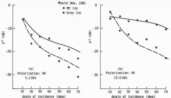
Fig. 4. Theoretical angular variations of σO of multi-year ice and first-year ice. The model parameters and experimental data are the same as those used in Figure 3.
Model behavior
The ranges of σo for multi-year and first-year ice were calculated by adjusting the model parameters within the reported ranges of values. From these ranges of σo, optimum radar parameters for sea-ice monitoring of two major ice types were defined to the extent possible with present knowledge.
As temperature changes, the dielectric constant of sea ice changes, although the exact dependence has yet to be determined. The temperature change also causes a change in the Fresnel reflection coefficient, resulting in a variation of σO of about 3 dB (Reference KimKim, unpublished). The change in the imaginary part of the dielectric constant due to temperature variation causes the volume-scattering characteristics of multi-year ice to change. The σO of multi-year ice can vary by as much as 6 dB (Reference KimKim, unpublished) under different temperature conditions.
The small-scale surface roughness plays an important role in determining the σO of first-year as well as multi-year ice. Both the density and size of air bubbles in multi-year ice have a significant impact on σO (< 3 dB and < 10 dB, respectively).
Frequency. Figure 5 shows the ranges of theoretical σO for multi-year and first-year ice under various conditions. The selected limiting values of the parameters are shown in the caption of this and subsequent figures. The lowest curve (1) is for smooth-surfaced first-year ice when salinity and temperature are low. As either the salinity or temperature increases, the dielectric constant increases. The next curve (2) is for first-year ice with a medium-rough surface and increased salinity and temperature. Curve (3) is for multi-year ice with a medium-rough surface and small air bubbles when the temperature is low. The highest curve (4) is for rough-surface multi-year ice with larger air bubbles and zero salinity, which cause a larger volume-scattering contribution due to decreased absorption loss.

Fig. 5. Theoretical σO for multi-year ice and first-year ice for θ = 40°. The ranges of values illustrated represent various limiting cases for model parameters.
-
First year ice: (1) smooth (σ = 0.15. l = 8.9 cm), S = 8°/00, T = −25° C; (2) medium rough (σ = 0.37. l = 8.5 cm), S = 10°/00. T = −15 ° C.
-
Multi-year ice: (3) medium-rough surface (σ = 0.37, l = 8.5 cm), S = 0.6°/00, T = −20° C, ρ = 0.75 g/cm3, air-bubble diameter = 1.6 mm, bubble layer = 20 cm. (4) rough surface (σ = 0.81, l = 8.2 cm), S = 0°/00, T = −15° C, ρ = 0.75 g/cm3, air-bubble diameter = 2 mm, bubble layer = 50 cm.
The effect of higher temperatures is to increase the σ° of first-year ice (surface scattering dominant) and to decrease the σO of multi-year ice (volume scattering dominant for frequencies higher than about X-band. Therefore, as temperatures increase, the difference in σO between first-year and multi-year ice decreases.
Figure 5 shows that, for nearly all frequencies considered, there is a difference in σO between multi-year and first-year ice. It can also be seen that higher frequencies give better discrimination.
In Figure 6 the model parameters are further varied to include very rough first-year ice with high salinity and temperature (curve (2)). Lossier multi-year ice with higher salinity and temperature than in curve (3) of Figure 5 is shown as curve (3) of Figure 6; multi-year ice with a rough surface, larger air bubbles, and zero salinity is plotted as curve (4) of Figure 6. In these cases, a large overlap between the σO values for first-year and multi-year ice can be seen except above 17 GHz. Unless the frequency is high enough, there can be confusion between first-year ice with a very rough surface and multi-year ice with small air bubbles, since surface roughness is the major factor in determining the σO of first-year ice.

Fig. 6. Theoretical σO for multi-year ice and first-year ice for θ = 40°. The ranges of values illustrated represent various limiting cases for parameters.
-
First-year ice: (1) smooth (σ = 0.15, l = 8.9 cm), S = 8°/00, T = – 25° C; (2) rough (σ = 0.81. l = 8.2 cm), S = 12‰, T = –5° C.
-
Multi-year ice: (3) medium-rough surface (σ = 0.37, l = 8.5 cm), S = 0.7°/00, T = –5°C, ρ = 0.75 g/cm3, air-bubble diameter = 1.6 mm, bubble layer = 20 cm; (4) rough surface (σ = 0.81, l= 8.2 cm), S = 0‰, T = –5° C, ρ = 075g/cm3, air-bubble diameter = 2.5 mm, bubble layer = 50 cm.
In Figure 6 the model parameters are further varied to include very rough first-year ice with high salinity and temperature (curve (2)). Lossier multi-year ice with higher salinity and temperature than in curve (3) of Figure 5 is shown as curve (3) of Figure 6; multi-year ice with a rough surface, larger air bubbles, and zero salinity is plotted as curve (4) of Figure 6. In these cases, a large overlap between the σO values for first-year and multi-year ice can be seen except above 17 GHz. Unless the frequency is high enough, there can be confusion between first-year ice with a very rough surface and multi-year ice with small air bubbles, since surface roughness is the major factor in determining the σO of first-year ice.
In no sense are the ranges shown in Figure 6 the absolute ranges of σO for multi-year and first-year ice. Only small-scale roughness (surface-height standard deviation less than a wavelength) was considered, and the effect of large-scale roughness (larger than a wavelength) caused by ridges, hummocks and melt ponds was neglected. The full ranges of surface roughness for multi-year and first-year ice have never been determined. Moreover, the distribution of sizes of air bubbles is in question. Temperatures above −5° C, where the dielectric constant of sea ice increases rapidly, were not considered.
The presence of snow-cover increases the backscatter from smooth first-year ice, resulting in a rise in the overall level of curves labeled (1) in Figures 5 and 6. The effect of snow-cover is more pronounced at higher frequencies (Reference Onstott, Onstott, Moore and WeeksOnstott and others, 1979) but the influence of snow-cover on frequency response of σO has not been established.
With all of these limitations, and for surface temperatures lower than −5° C, higher frequencies can be stated to be better than lower ones in discriminating multi-year from first-year ice.
Incidence angle. The theoretical angular response of multi-year and first-year ice at 5 and 15 GHz is shown in Figure 7. The σO of first-year ice decreases rapidly with increasing incidence angle but that of multi-year ice decays more slowly because of the presence of volume scattering. Therefore, in terms of discrimination capability, incidence angles greater than 30° or 40° are to be preferred.

Fig. 7. Theoretical angular variations of σO of multi-year ice and first-year ice. The model parameters are the same as those used in Figure 5.
As the model parameters are varied further to include very rough first-year and lossier multi-year ice, the overlap between scattering from the two ice types occurs for all the incidence angles, as illustrated in Figure 8. The theoretical model bounds all the measurements shown except one. As mentioned in the previous section, the boundaries are not the absolute limits and further study is needed. However, the fact that all first-year-ice measurements at incidence angles greater than 10° lie below the lowest multi-year-ice measurements is encouraging.

Fig. 8. Theoretical boundaries of σO for multi-year ice and first-year ice. The model parameters are the same as those used in Figure 6, Several reported measurements are shown. Except for Reference Gray, Gray, Hawkins, Livingstone, Arsenault and JohnstoneGray’s (1982) case of multi-year ice, all lie within the boundaries. Solid points are first-year ice.
Polarization. Both the radiative transfer and semi-empirical volume-scatter models predict a slightly higher
The radiative-transfer volume-scatter model can explain the cross-polarized σO for multi-year ice (Reference KimKim, unpublished),
Conclusions
This paper provides a summary of experimental findings reported to date and, using a reasonable set of model parameters, compares them with theoretical models that match the data sets. By adjusting, within reported ranges, the model parameters for σO, roughness, and air-bubble size, the possible ranges of σ° for multi-year and first-year ice are calculated. This shows that the best radar parameters for sea-ice monitoring are: (1) X- or Ku-band frequencies (higher frequencies were not considered), and (2) incidence angles equal to or greater than 30°. No specific resonances were found that might favor any frequency or incidence angle. The theoretical findings agree with the general experimental conclusions.
The optimum polarization could not be selected. This was due in part to the lack of reliable cross-polarized data for the whole frequency range considered, and in part to the inability of the first-order surface-scattering model to explain the polarization dependence of backscatter from sea ice.
The theoretical calculations and models presented in this paper were restricted to surface temperatures below −5°C, so the models are not expected to be valid during the melt season, when ice properties change drastically.
The physical and electrical characteristics of ice and snow need further study in order to refine the models. The important parameters should be: (1) the ranges of values of small-scale roughness for multi-year and thinner types of sea ice; (2) the behavior of the dielectric constant (especially the imaginary part) or the upper parts of multi-year ice; and (3) the distribution of air-bubble diameters in the various layers of multi-year ice found in different areas of the Arctic.


