


1. Introduction
1.1. Ubiquity of shear instabilities
Shear instabilities are ubiquitous at a range of scales and for a range of applications, from extragalactic jets (Lobanov & Zensus Reference Lobanov and Zensus2001) and interstellar clouds (Berné, Marcelino & Cernicharo Reference Berné, Marcelino and Cernicharo2010), the solar atmosphere and geomagnetosphere (Johnson, Wing & Delamere Reference Johnson, Wing and Delamere2014; Mishin & Tomozov Reference Mishin and Tomozov2016), to the Earth's ocean waves and clouds (Smyth & Moum Reference Smyth and Moum2012; Houze Reference Houze2014). At air–liquid interfaces, shear instabilities of the Kelvin–Helmholtz type can initiate a chain of events creating sheets, themselves then coupled with Rayleigh–Taylor or Rayleigh–Plateau family types of instabilities (Helmholtz Reference Helmholtz1868; Kelvin Reference Kelvin1871; Rayleigh Reference Rayleigh1879), that culminate in fragmentation, forming emitted droplets of a range of sizes and speeds (Villermaux Reference Villermaux2007, Reference Villermaux2020; Eggers & Villermaux Reference Eggers and Villermaux2008; Wang & Bourouiba Reference Wang and Bourouiba2018; Wang et al. Reference Wang, Dandekar, Bustos, Poulain and Bourouiba2018).
Recall that, in the classical Kelvin–Helmholtz (KH) instability with sharp discontinuity, for constant/steady shear and using normal modal analysis with small-amplitude interfacial waves of the form  ${\rm e}^{{\rm i}(kx-\omega t)}$, the dispersion relation is
 \begin{equation} \omega^2=\left[gk\left(\frac{\rho_1-\rho_2}{\rho_1+\rho_2}\right)+\frac{\sigma k^3}{\rho_1+\rho_2}\right]-\frac{k^2(U_1-U_2)^2\rho_1\rho_2}{(\rho_1+\rho_2)^2},\end{equation}
where  $i$ is the imaginary unit number, $x$ is the coordinate whose axis aligns with the mean interface, $t$ is time, $k$ is the wavenumber, $\omega (k)$ is the wave frequency, $g$ is the gravitational acceleration, $\sigma$ is the surface tension, $\rho _{1,2}$ and $U_{1,2}$ are the density and imposed shear velocity in the lower and upper fluid, respectively. As formulated above, in (1.1), a flow configuration is stable if $\omega$ is real and unstable if $\omega$ is imaginary. The role of viscosity and a spatially varying, but constant in time, velocity profile within a thin shear layer has received extensive attention since Rayleigh, for example, how viscosity would give rise to (Yih Reference Yih1967; Hinch Reference Hinch1984) or shift the selection of the fastest growing mode (Villermaux Reference Villermaux1998; Yecko, Zaleski & Fullana Reference Yecko, Zaleski and Fullana2002; Boeck & Zaleski Reference Boeck and Zaleski2005). Moreover, most theoretical and numerical studies of such KH type canonical shear instabilities in a range of systems consider parallel shear flows with a focus on either constant velocity, or in the following references, for example, strictly oscillatory velocities in time (Kelly Reference Kelly1965; Lyubimov & Cherepanov Reference Lyubimov and Cherepanov1986; Khenner et al. Reference Khenner, Lyubimov, Belozerova and Roux1999; Poulin, Flierl & Pedlosky Reference Poulin, Flierl and Pedlosky2003; Yoshikawa & Wesfreid Reference Yoshikawa and Wesfreid2011). In these studies, it is established that both modal and parametric instabilities can occur in oscillatory flows. In the former case, the Kelvin–Helmholtz instability (KHI) threshold is lowered because oscillations reduce the effective interface stiffness.
1.2. Ubiquity of impulsive flows, and importance for respiratory violent exhalations
However, in a range of environmental and physiological settings the liquid–air interface perturbation is driven by intrinsically impulsive, and often asymmetric in time, flow profiles. For example, violent exhalation processes last about 100–200 milliseconds for sneezes and 200–300 milliseconds for coughs (Bourouiba, Dehandschoewercker & Bush Reference Bourouiba, Dehandschoewercker and Bush2014; Scharfman et al. Reference Scharfman, Techet, Bush and Bourouiba2016), with peak velocities upwards of  $O(10)$–
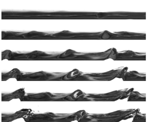
 $O(100)$ metres per second (Han, Weng & Huang Reference Han, Weng and Huang2013; Bourouiba Reference Bourouiba2021b). Sample human impulse cough flows obtained from spirometry are shown in figure 1(a) (Bourouiba Reference Bourouiba2021b). The interaction between the impulsive violent pulmonary airflows and the mucosalivary fluid lining creates a rich class of interfacial destabilization mechanisms, ultimately culminating in fluid fragmentation. For example, the early stage of liquid lining destabilization and fragmentation is shown in figure 1(b) in a mimic trachea size cylinder subject to a mimic cough impulse of the type shown in figure 2(a). The resulting fragmentation shapes the formation of mucosalivary fluid droplets, of a continuum of sizes, that can encapsulate and transport pathogens in exhalation turbulent puff clouds (Bourouiba et al. Reference Bourouiba, Dehandschoewercker and Bush2014; Bourouiba Reference Bourouiba2020, Reference Bourouiba2021b) as seen at the exit of the respiratory tracts in figure 1(c).

Figure 1. (a) Flow rate measurements for unsteady violent exhalations such as coughs that drive mucosalivary liquid fragmentation (Bourouiba Reference Bourouiba2021b). (b) Images of a thin layer of liquid being sheared, and consequently fragmented, by an unsteady impulsive parallel airflow. The flow direction is right to left and its temporal velocity profile is discussed in figure 19 (Impulse B). (c) Visualization of the resulting fragmentation and emission of mucosalivary liquid from the respiratory tract during a violent exhalation (Scharfman et al. Reference Scharfman, Techet, Bush and Bourouiba2016; Bourouiba Reference Bourouiba2021b). The scale bars shown in (b) and (c) refer to 1 mm and 1 cm, respectively; and the time origin from onset of airflow impulse for (b) and (c) are distinct.

Figure 2. (a) Canonical flow profile  ${\rm \Delta} U$ for an idealized typical cough. The maximum and time-averaged flow speeds are 10 m s $^{-1}$ and 5 m s $^{-1}$, respectively. Thick lines are used to label portion of the profile that is KH unstable with respect to wavelength $\lambda = 2$ cm. (b) Classical KH instability dispersion map, (1.1), plotted for liquid–air interface with flow speeds ${\rm \Delta} U=5,10$ m s $^{-1}$.
Continuing with the example of respiratory impulsive flows, attention has been paid to the role of flexible walls in mucous clearance, with Scherer & Burtz (Reference Scherer and Burtz1978) conducting mimic cough experiments where sudden blasts of air were introduced into a flexible tube lined with a Newtonian liquid layer. Large-amplitude waves on the air–liquid interface and droplets breaking were observed. Attention has also been given to the role of rheology with King, Brock & Lundell (Reference King, Brock and Lundell1985) and Basser, McMahon & Griffith (Reference Basser, McMahon and Griffith1989) using a similar impulse release approach in rigid channels lined with non-Newtonian and yield stress liquids aiming to mimic some aspects of mucous. Such impulse release on a liquid lining in a square channel was recently revisited with experiments and simulations with liquid lining (Kant et al. Reference Kant, Pairetti, Saade, Popinet, Zaleski and Lohse2022) with a focus on the overall droplet sizes generated.
1.3. Limited understanding of the role of unsteadiness and study questions
Yet, despite these efforts and attention, we still understand little about how the properties of the unsteadiness of the rapidly changing pulse governs the destabilization of the interface on the time scale of the pulse. Equation (1.1) with constant  ${\rm \Delta} U=U_2-U_1$ is not applicable for an unsteady, let alone impulsive flow to gain insights on the interface stability. To derive insights on how the instability is selected and develops in such flows, one could take the instantaneous velocity at a given time, and using (1.1) assess stability given a wavelength of interest.
For example, figure 2(a) gives an idealized impulsive temporal profile of a cough flow in the upper respiratory tract corresponding to the measurements of figure 1(a). Taking  $\lambda =2$ cm, figure 2(a) shows the thick black portion of the unsteady flow profile that would be classically KH linearly unstable. More typically, one could take either the peak or the mean, time-averaged, velocities (5 and 10 m s $^{-1}$, respectively, in figure 2a) to examine stability maps (e.g. Yoshikawa & Wesfreid Reference Yoshikawa and Wesfreid2011; Fraser, Cresswell & Garaud Reference Fraser, Cresswell and Garaud2022), such as that shown in figure 2(b). However, this map shows that, doing so, in fact leads to misleading insights with contradicting stability results between these two characteristic velocities: the choice of average velocity would suggest that the interface would remain stable, while the peak velocity would suggest that instability can occur. These motivating examples lead to the following questions:
(i) Can impulsiveness lead to counterintuitive results, where destabilization is enhanced or hindered due to the transient nature of the impulse, when compared with the expected outcome from a steady classical KH stability analysis, where some instantaneous or integrated properties of the impulse flow are used?
(ii) When mapping the canonical shear instability framework associated with a constant imposed shear flow to an interfacial perturbation subjected to an impulse, what physical quantity or property of the impulse matters to trigger instability, and on which time scale? For example, should one reason with peak and/or averaged flow velocities, total energy injection or something else?
(iii) How does the interface evolve during such impulsive perturbations? In particular, given the very transient nature, how does the time scale of perturbation growth compare with the impulse time scale to shape transient vs asymptotic amplitude growth and transition from linear to nonlinear regimes of perturbations?
(iv) How does the time scale of instability onset compare with that of the impulse imposed? For example, does the instability develop always during the ramp up of the impulse, or can it develop during ramp down or even after end of the impulse?
1.4. Study approach, assumptions and outline
To address these questions, we use a combination of linear and nonlinear theoretical and numerical analyses combined with experiments. To crystalize the essential role of unsteadiness, we focus our analysis and simulations on a configuration of reduced complexity in which a two-dimensional air-on-liquid interface is subjected to spatially uniform, but time-varying velocity profiles that mimic respiratory flow impulses such as shown in figure 1(a) or idealized forms such as that shown in figure 2(a). In our present study, we consider only the case of the liquid layer, of density  $\rho _1$, below the air layer, of density $\rho _2$, so as to focus on the shear destabilization effect. We also consider the two phases to be incompressible, immiscible, inviscid and subject to gravity and surface tension. While discontinuity of velocity is typically regularized by viscosity, which has received extensive attention (Rayleigh Reference Rayleigh1879; Betchov & Szewczyk Reference Betchov and Szewczyk1963; Villermaux Reference Villermaux1998; Marmottant & Villermaux Reference Marmottant and Villermaux2004; Boeck & Zaleski Reference Boeck and Zaleski2005), we here chose to focus on the inviscid regime as the simplest canonical unsteady configuration enabling us to gain a focused insight into the dominant role of sharp time variation rather than mixing spatial and temporal variations. Moreover, the error committed by neglecting viscous effects is reduced in flows of high Reynolds numbers (Villermaux Reference Villermaux1998; Boeck & Zaleski Reference Boeck and Zaleski2005) and short duration, such as those associated with violent exhalations (Bourouiba Reference Bourouiba2021a). Furthermore, we verify qualitatively the insights gained by our theory and modelling with an experimental configuration (§ 4) that includes not only viscosity but also confined geometry.
We focus on the interfacial response to impulsive shearing specifically accounting for the flow history and its cumulative effects. We achieve this by formulating the evolution of a sinusoidally perturbed interface as an impulse-driven initial value problem. We solve also the linearized flow equations based on the framework of Kelly (Reference Kelly1965), where the amplitude of the interface perturbation is governed by an ordinary differential equation (ODE). We simulate the nonlinear behaviour of the interface as a vortex sheet using a boundary integral method that extends the development of Pullin (Reference Pullin1982) and Baker, Meiron & Orszag (Reference Baker, Meiron and Orszag1982) explicitly to accommodate unsteady background flows. This differentiates the present work from previous studies for the motion of vortex sheets (Krasny Reference Krasny1986; Rangel & Sirignano Reference Rangel and Sirignano1988; Hou, Lowengrub & Shelley Reference Hou, Lowengrub and Shelley1997; Sohn, Yoon & Hwang Reference Sohn, Yoon and Hwang2010) where steady parallel shear flows were considered.
Our results show that the amplitude of a gravity–capillary wave (GCW) initially at the interface can be amplified by the imposed impulse shear flow, even if such flow is classically KH stable. We find that we could classify the stability into four regimes discussed in § 2.4 after introduction of all notations and framework. If the impulse duration is short relative to the interface's GCW natural oscillation period, the maximum amplitude can be reached after the end of the impulse. While, if the two time scales are comparable, the maximum amplitude can occur before the end of the impulse. Moreover, we show that if sufficient transient perturbation growth can be generated by the impulse, a transition from persistent oscillations to wave breaking can occur independent of the classical KH stability framework applied to an instantaneous value of the impulse velocity.
We next discuss, in § 2, the linearized potential flow theory where we introduce the unperturbed interface base flow and the impulsive profiles used as canonical functional forms of violent exhalations. We obtain the ODE system that governs the amplitude of a single-mode perturbation around the base flow in the linear regime and derive both numerical and asymptotic solutions for impulses of short and long durations with respect to the period of the unperturbed interface oscillation. In § 3 we discuss the nonlinear analysis for the impulse-driven interfaces and derive the governing equations using a boundary integral as an integro-differential equation (IDE) system. We present the simulation results for amplified waves, breaking waves and stability transition as a function of the flow impulse's strength and duration. In § 4, we support our findings experimentally in a configuration that accounts for viscosity and confined trachea-like geometry.
2. Linearized potential flow theory and simulations
To gain fundamental insights, we first explore the simplified theory of linearized potential flow. We consider the unbounded two-dimensional motion at a liquid–gas interface, under immiscible, incompressible and inviscid flow assumptions (see figure 3 for a schematic). The  $x$-axis labels the horizontal direction along the mean interface, while the $y$-axis labels the vertical direction aligned with gravity, $g$ pointing in the negative direction. The interface shape is prescribed by $y=\eta (x,t)$ and is periodic in the $x$-direction with wavelength $\lambda$. The subscript $j$ labels the lower (liquid, $j = 1$) and upper (gas, $j=2$) phases, with densities, $\rho _j$, pressures $p_j$, velocity potentials $\phi _j$ and velocity fields $\boldsymbol {u}_j=\boldsymbol {\nabla }\phi _j=(u_j, v_j)$. We define the perturbation of the interface relative to a spatially uniform but temporally unsteady parallel base flow in the positive $x$-direction of magnitude ${U}_j(t)$, over the undisturbed flat interface $\eta =0$, with examples given in figure 4(b) and introduced formally in § 2.3.

Figure 3. Schematic of a two-dimensional interface separating two fluids of different densities  $\rho$. A Cartesian coordinate system is used to specify the interface location $\eta$. Unsteady parallel shear flows $U(t)$ are imposed in each fluid region defined by an initial interfacial perturbation of size $\eta _0$. Gravitational acceleration $g$ and surface tension $\sigma$ are labelled.

Figure 4. (a) Schematic of the temporal profile of a canonical airflow impulse  $U_2(T)$. A stability line is drawn at $U_2=M^{-1}$, indicating that portions of the flow impulse above the stability line ( $U_2>M^{-1}$, shaded) is KH unstable in the classic linear theory. Here, $M$ is the effective impulse strength defined in (2.13). (b) Examples of the canonical pulse velocity profiles given formally in (2.16), where, here, the common impulse peak time is $\tau _1/\tau _p=0.006$. In both panels, normalized time unit $T = \tau /\tau _p$ is used.
Unless otherwise specified, we use dimensionless variables, non-dimensionalized using the length scale  $\lambda$, velocity scale $U_m=\max _{t\geq 0}U_j$ and density scale $(\rho _1+\rho _2)/2$, leading to a unit time $\lambda /U_m$ and potential $\lambda U_m$. As a result, the two-phase flow system is governed by the non-dimensional continuity and Bernoulli equations
 \begin{gather} \nabla^2 \phi_j=0, \end{gather}
 \begin{gather}\frac{p_j}{\rho_j}+\frac{1}{2}(u_j^2+v_j^2) +\frac{y}{{Fr}^2}+\frac{\partial \phi_j}{\partial t}=F_j(t), \end{gather}
where
 \begin{equation} {Fr}=\frac{U_m}{\sqrt{g \lambda}},\end{equation}
is the Froude number, and  $F_j(t)$ is an arbitrary function of time. Being a material separation line, the interface must also satisfy the kinematic and dynamic conditions
 \begin{gather} \partial_t\eta+\lim_{y\to \eta}u_j\partial_x\eta=\lim_{y\to \eta}v_j, \end{gather}
 \begin{gather}\lim_{y\to \eta^+}p_2-\lim_{y\to \eta^-}p_1=\frac{\kappa}{We}=\frac{\partial^2_x \eta}{{We}(1+\partial_x\eta)^{3/2}}, \end{gather}
where  $\kappa$ is the interfacial curvature and
 \begin{equation} {We}=\frac{(\rho_1+\rho_2)U_m^2\lambda}{2\sigma}\end{equation}
is the Weber number and  $\sigma$ is the surface tension.
2.1. Flow velocities of the air impulse and resulting unsteady base state in the liquid phase
The temporal variation of the air impulses  $U_2(t)$ considered is specified in § 2.3 in detail. From such temporal functional forms, we can obtain the parallel flow velocity and pressure fields in the liquid phase by solving (2.1b) and (2.3b) for a flat interface $\eta =0$. Following Kelly (Reference Kelly1965) we obtain the unsteady base flow in the liquid phase
 \begin{equation} U_1(t)=\frac{1-A}{1+A}\int {U}'_2(t)\, {\rm d} t,\end{equation}
where
 \begin{equation} A=\frac{\rho_1-\rho_2}{\rho_1+\rho_2},\end{equation}
is the Atwood number, and the prime symbol denotes time derivative. Here,  $A>0$ with $U_1(0)=0$ to ensure a vanishing integration constant. Substituting $(u_j, v_j)=(U_j, 0)$ and $\phi _j=x U_j$ into (2.1b) leads to the pressure profile in phase $j$
$j$
 \begin{equation} p_j=\rho_j\bigg(F_j-\frac{|\boldsymbol{u}_j|^2}{2}- \frac{y}{{Fr}^2}-\frac{\partial\phi_j}{\partial t}\bigg)\equiv P_j. \end{equation}
We are now ready to examine the perturbation of this base state next.
2.2. Linearized equations
Next, we follow Kelly (Reference Kelly1965) and solve for the linearized equations. This begins with a single Fourier mode perturbation of small amplitude  $\epsilon \ll 1$ and wavenumber $k=2{\rm \pi}$ to the originally flat interface at $t=0$. The resulting governing equations subject to the modelled velocity impulse take the form
 \begin{equation} f_j(x,y,t)=f_{j,0}(x,y,t)+\tilde{f}_{j}(y,t)\, {\rm e}^{{\rm i}kx}\epsilon+O(\epsilon^2),\end{equation}
where  $f$ is one of our variables $\phi,u,p,\eta$ and $f_{j,0}$ is the corresponding base state solution: $\phi _{j,0}=x U_j$, $p_{j,0}=P_j$ (2.7) and $\eta _0=0$. Note that we focus on perturbations with explicit $x$-dependence of the form ${\rm e}^{{\rm i}kx}$ and generally unspecified temporal dependence in $\tilde {f}_{j}(y,{t})$. Substituting (2.8) into (2.1) and (2.3) yields the linearized equations for $\tilde {f}$ at $O(\epsilon )$ that reduce to
 \begin{equation} \tilde{\phi}_j=\frac{({-}1)^{j+1}}{k}\left(\frac{{\rm d} \tilde{\eta}}{{\rm d} t} +{\rm i}kU_j\tilde{\eta}\right)\exp({({-}1)^{j+1}k y}), \end{equation}
where the interface displacement,  $\tilde {\eta }$, viewed in the centre of mass frame as
 \begin{equation} \tilde{\eta}(t)=\hat{\eta}(t)\exp\left(-\frac{{\rm i} k}{2}\int_0^t [\rho_1U_1({t'})+\rho_2 U_2({t'}) ]\,{\rm d} {t'}\right),\end{equation}
is governed by the following ODE:
 \begin{equation} \frac{{\rm d}^2\hat{\eta}}{{\rm d} t^2}+\left[\frac{k A }{{Fr}^2}+\frac{k^3}{2 {We}}-\frac{k^2(1-A^2 )}{4}(U_1-U_2)^2\right]\hat{\eta}=0, \end{equation}
equivalent to the result of Kelly (Reference Kelly1965).
Using (2.5) to eliminate  $U_1$, from (2.11) it is clear that the velocity impulse in the gas phase drives interfacial perturbation amplitude growth, whereas gravity and surface tension are stabilizing. Conveniently, we introduce the rescaled time
 \begin{equation} \tau=t \sqrt{\frac{k A }{{Fr}^2}+\frac{k^3}{2 {We}}} = t\varOmega,\end{equation}
and combine this competition in an effective flow strength  $M$, defined as
 \begin{equation} M=M({Fr},{We},A;k)\equiv\frac{tkA}{\tau}\sqrt{\frac{1-A}{1+A}},\end{equation}
where  $M$, a dimensionless parameter, measures the relative strength of the imposed gas flow $U_2$ opposing the restoring forces. As such, (2.11) simplifies to
 \begin{equation} \frac{{\rm d}^2\hat{\eta}}{{\rm d} \tau ^2}+[1-M^2U_2(\tau)^2]\hat{\eta}=0.\end{equation}
We recover that, for constant  $U_2$ and for $MU_2>1$, $\hat {\eta }$ exponentially grows, as expected when recovering the classical steady KH instability. For a time-varying impulse $U_2(\tau )$, we thereafter refer to the interval of time over which $M U_2(\tau )>1$ as classically KH unstable and that for which $M U_2(\tau )<1$ as classically KH stable, i.e. with $\hat {\eta }$ oscillatory in nature (see figure 4a).
Markedly, using (2.2) and (2.4), we find that  $M$ is maximized at the physical wavelength $\lambda$
 \begin{equation} \lambda=\lambda_0=2{\rm \pi}\sqrt{\frac{\sigma}{(\rho_1-\rho_2)g}},\end{equation}
independent of the flow velocity. In other words, at the capillary length, below which surface tension dominates gravity,  $\lambda _0$, the interface is easiest to destabilize for any imposed flow $U_2(\tau )$. We are now ready to introduce formally the canonical impulsive flow profiles we consider in this study.
2.3. Canonical impulsive flows considered for the air layer,  $U_2(t)$

We examine analogue violent exhalation flows consistent with observations (King et al. Reference King, Brock and Lundell1985; Basser et al. Reference Basser, McMahon and Griffith1989; Bourouiba et al. Reference Bourouiba, Dehandschoewercker and Bush2014; Bourouiba Reference Bourouiba2021b) as seen in figure 1(a). To do so, we consider canonical impulsive flows  $U_2(t)$ shown in figure 4(b) and given by
 \begin{gather} U_2^S(t;t_1,t_2)\equiv H(t-t_1)-H(t-t_2),\quad \text{Step profile}, \end{gather}
 \begin{gather}U_2^L(t;t_1,t_2)\equiv\frac{t}{t_1}[1-H(t-t_1)]+ \frac{t_2-t}{t_2-t_1}[H(t-t_1)-H(t-t_2)], \quad \text{Linear profile}, \end{gather}
 \begin{gather}U_2^E(t;t_1,\beta)\equiv\frac{t}{t_1}[1-H(t-t_1)] +{\rm e}^{-({t-t_1})/{\beta}}H(t-t_1), \quad \text{Exponential profile}, \end{gather}
 \begin{gather}U_2^G(t;t_1,\mu)\equiv\frac{t}{t_1}[1-H(t-t_1)] +{\rm e}^{-{(t-t_1)^2}/{\mu}}H(t-t_1), \quad \text{Gaussian profile}, \end{gather}
where the superscripts  $S$,
$S$,  $L$,
$L$,  $E$ and $G$ denote the abbreviated profile names, $H(t)$ is the Heaviside function with $H(0)=1$.
We choose the three parametrized functions to be piecewise monotonic with properties that  $U_2(0)=U_2(\infty )=0$ and $\max _{t\geq 0}U_2(t)=1$, in order to capture the rise and decay stages of the impulses. The step profile $U_2^S$ features discontinuities at $t=t_1>0$ and $t=t_2>t_1$ that turn the driving impulse on and off, respectively. The continuous profiles, $U_2^{L,E, G}$, share the same linear increase for $0\leq t\leq t_1$ to reach peak velocity but differ in the subsequent velocity decay: $U_2^L$ linearly decreases for $t_1< t< t_2$, $U_2^E$ exponentially decays at a rate $\beta$ and $U_2^G$ has a Gaussian decay of variance $\mu >0$ for $t>t_1$.
The characteristic parameters of each of the canonical airflow impulses  $U_2(t)$, given in (2.16), are further detailed in table 1. In particular, this includes the effective non-dimensional impulse duration $\tau _d$ defined for the exponential ( $E$) and Gaussian impulses ( $G$) in terms of a small threshold value $0< d\ll 1$ such that
 \begin{equation} \tau_d = t_d \varOmega =\max \{\tau: U_2^{E,G}(\tau)=d\}.\end{equation}
In the cases of the linear ( $L$) and step ( $S$) impulses, clearly $\tau _d = \tau _2$ (see table 1).
Table 1. Characteristic parameters of the four velocity impulse profiles specified in (2.16) and shown with examples in figure 4(b). A sharp cutoff duration,  $t_2$, or non-dimensional $\tau _2 = t_2 \varOmega$ (see (2.12)) is only strictly defined for the step ( $S$) and linear ( $L$) profiles. Thus, we introduce the small parameter $d$ and impulse duration $\tau _d$, defined by (2.17) for the exponential ( $E$) and Gaussian ( $G$) profiles. The approximate expressions for the total action, $S_\infty$, defined in (2.21), and the impulse's profile action correction factor $\alpha$, defined in (2.29), are computed in the limit of $\varepsilon =\tau _1/\tau _d\to 0$. We chose $d = 0.01$ for all the numerical results we display in this study. Moreover, we introduced time normalized with respect to the interface natural oscillation, $\tau _p = 2{\rm \pi} : T = \tau /\tau _p$, with associated normalized characteristic times of the impulse $T_1 = \tau _1/\tau _p$, $T_2 = \tau _2/\tau _p$ or $T_d = \tau _d/\tau _p$.

Note that our focus is on dramatic transient effects and so we chose rapidly linearly increasing functional forms up to their maximum velocity value reached at  $t_1$; with $t_1\ll t_d$ to ensure that the rise time is significantly shorter than the total duration of the impulse. This choice was done to remain consistent with physiological observations. However, we a posteriori also confirm these choices do not affect the amplification of the interface for short impulses, and in fact such choices maximize amplification for long impulses as discussed in § A.1. Finally, we denote the characteristic times of these impulses in their non-dimensional forms as $\tau _1 = t_1\varOmega$, $\tau _2 = t_2\varOmega$ (see 2.12 for definition of $\varOmega$) and we examine our results, for the most part, in the limit of $\varepsilon =\tau _1/\tau _d\to 0$. We also introduce another characteristic time, normalized with respect to the interface natural oscillation, $\tau _p = 2{\rm \pi}$, with associated normalized characteristic impulse functional form times $T_1 = \tau _1/\tau _p$, $T_2 = \tau _2/\tau _p$ or $T_d = \tau _d/\tau _p$.
2.4. Stability regimes: framing of the analysis and results
With effective impulse strength  $M$ and its normalized duration ( $T_2 = \tau _2/\tau _2$ or more generally $T_d=\tau _d/\tau _p$ discussed in table 1) that vary independently, we identify that representative exhalation impulses can be categorized into four stability regimes shown in figure 5. Each regime generates qualitatively distinct interface responses. We will use the framing of this regime map to discuss the details of our linear analysis (presented in § 2) and nonlinear analysis (§ 3). First, we will show with linear theory that, in the limit of very short impulses $T_2 \to 0$, regardless of the impulse strength, $M$ (regimes I and IV), the response of the interface is independent of the details of the impulse's functional form and is entirely determined by a quantity analogous to cumulative imparted energy: the total action, $S_{\infty }$ defined by (2.21) in § 2.6. Transient linear growth of the interface's amplitude can lead to maximal amplification reached in the first oscillation of the interface, despite the impulse being considered classically KH stable at all times. As the impulse lengthens and for strong impulses in the limit $M\to \infty$ (regime III), we show that we recover an increasing dependence of the interface's response on the impulse's functional form, in addition to the time-varying injected action $S$. In the extreme part of this limit, in fact, we recover the classical KH linear instability exponential growth, expected to subsequently transition to nonlinear fragmentation. Next, and transiting to both nonlinear and linear theory and simulations, we will show that the behaviour of the interface in the intermediate regimes I ( $M\gg 1, T_2\ll 1$) and II ( $M\lesssim 1, T_2\gtrsim 1$) depend on the cumulative effect of the GCW amplification through the duration of the impulse imposed. As a result, we have transition from sustained GCW to nonlinear wave breaking, revealed fully when considering nonlinear effects in § 3. With this framing in mind, we next present the analytical and numerical results from our linear analysis, starting with the importance of considering non-modal transient growth.

Figure 5. Schematics for flow impulses  $U_2^L$ of varying effective strength $M$ and normalized duration $T_2$. Four stability regimes are given as regime I, $M\gg 1, T_2\ll 1$; regime II, $M\lesssim 1, T_2\gtrsim 1$; regime III, $M\gg 1, T_2\gtrsim 1$; and regime IV, $M\lesssim 1, T_2\ll 1$. In each case, a stability line is drawn at $U_2=M^{-1}$, indicating that portions of the flow impulse above the stability line ( $U_2>M^{-1}$, shaded) is KH unstable in the classic linear theory.
2.5. Non-modal transient growth and maximum growth in the limit of $U_2\equiv 1>M$

The initial condition required to integrate (2.14) is chosen to be one that corresponds to the normal mode of the form  $\hat {\eta }(\tau )={\rm e}^{-{\rm i}\omega \tau }$, where the instantaneous (complex) angular frequency is $\omega =\sqrt {1-M^2U_2(\tau )^2}$ evaluated $\tau = 0$. Since $U_2(0)=0$, we arrive at the following initial values:
 \begin{equation} \hat{\eta}(0)=1,\quad \hat{\eta}'(0)={-}i.\end{equation}
However, the normal mode does not solve (2.14) generally for  $\tau >0$ where $U_2$ and therefore $\omega$ are no longer constant (travelling wave solutions exist only for constant $U_2$ and $U_2M<1$). It is critical thus to focus on transient growth and associated maximum amplification.
We do so now in the limits of  $U_2\equiv 1>M$ and weak impulses with $M < 1$ (regimes IV and II), where we solve for the perturbation amplitude $\hat {\eta }$ and using the initial values (2.18a,b), leading to
 \begin{equation}
|\hat{\eta}(\tau)|^2=\frac{M^2\cos \left(2 \tau
\sqrt{1-M^2}\right)+M^2-2}{2M^2-2},\end{equation}
\begin{equation}
|\hat{\eta}(\tau)|^2=\frac{M^2\cos \left(2 \tau
\sqrt{1-M^2}\right)+M^2-2}{2M^2-2},\end{equation}
which oscillates between zero and a maximum value first obtained at  $\tau =\tau _m={\rm \pi} /(2\sqrt {1-M^2})$, given by $\eta _{max}=|\hat {\eta }(\tau _m)|=1/(1-M^2)>1$. Markedly, at least in the inviscid limit considered here, transient growth of the amplitude $|\hat {\eta }|$ is observed for the time interval $0\leq \tau <\tau _m$.
Although the growth rate is at most linear in this case (exactly linear if  $M=U_2=1$), the peak amplitude $\eta _{max}$ and time to maximum amplitude, $\tau _m$, both increase with increasing $M<1$ and approach infinity as $M\to 1$. In such unbounded limit, a transient growth (Kerswell Reference Kerswell2018) found for conventionally KH stable flows ( $M<1$) is also potentially capable of destabilizing the two-fluid interface. Indeed, it will be shown in § 3.3.3 that, with sufficiently large initial perturbation size $\epsilon$, nonlinear wave breaking can occur in the transient growth regime. This result complements the conventional understanding of linearized KH instability that is associated with exponential perturbation growth of normal modes.
2.6. Asymptotic solution for short impulses and importance of the action integral $S$

The ODE system (2.14) and (2.18a,b) for general  $M$ and $U_2$ can be readily solved using standard numerical methods and we discuss such numerical results in § 2.7. Here, we start by deriving an analytic solution that explicitly elucidates the effect of an impulsive $U_2$ on the interfacial evolution. An iterative perturbation method demonstrated in Bender & Orszag (Reference Bender and Orszag1999) is used in the following.
To begin, as  $t\to 0^+$, the leading-order behaviour of $\hat {\eta }$ is given by $\hat {\eta }=1+O(\tau )$. Substituting this limit into the second term of (2.14) allows the resulting equation to be explicitly integrated, producing the first-order approximate solution
 \begin{equation} \hat{\eta}(\tau)\approx \hat{\eta}_1(\tau)=1-i\tau-\frac{\tau^2}{2}+M^2\int_0^\tau S(\tilde{\tau}) \, {\rm d} \tilde{\tau}, \end{equation}
where  $S$ is the action integral
 \begin{equation} S(\tau)=\int_{0}^{\tau} U_2(\tilde{\tau})^2 \, {\rm d} \tilde{\tau}.\end{equation}
Note that, by further requiring sufficient decay of  $U_2(\tau )\to 0$ for large $\tau$, the integral $S(\tau )$ converges for large $\tau$; and we denote the limit $S_\infty =\lim _{\tau \to \infty }S(\tau )$, whose significance will be discussed in detail later.
The  $\hat {\eta }$ approximation derived in (2.20) improves on the limit $\hat {\eta }=1$ by including not only correction due to the initial first-order derivative, as expected in a power series, but also the integral of action $S$ that captures the air kinetic energy injected into the system. Further, because $\hat {\eta }_1$ is also explicit in $\tau$, it can be used again in (2.14) to obtain corrections of next order. Iterating this process thus leads to the exact series solution as follows:
 \begin{equation} \hat{\eta}(\tau)=\lim_{N\to \infty}\hat{\eta}_N(\tau)=1+\lim_{N\to \infty}\int_{0}^{\tau}\, {\rm d} \tilde{\tau} \sum_{n=1}^N \mathcal{L}_n(\tilde{\tau}), \end{equation}
where  $\hat {\eta }_N$ is the $N$th-order approximation, $\mathcal {L}_n$ is defined through the recursion relation
 \begin{equation} \mathcal{L}_{n}(\tau)=\int_{0}^{\tau} \left\{[M^2U_2 ({\tau_1})^2-1]\int_{0}^{\tau_1}\mathcal{L}_{n-1}(\tau_2) \, {\rm d} \tau_2\right\}\, {\rm d} \tau_1,\end{equation}
for  $n\geq 2$ and
 \begin{equation} \mathcal{L}_1(\tau)={-}i +\int_0^\tau [M^2 U_2(\tilde{\tau})^2-1]\, {\rm d} \tilde{\tau}={-}i - \tau + M^2 S(\tau). \end{equation}
The time derivative  $\hat {\eta }'$ follows immediately as $\hat {\eta }'(\tau )=\sum _{n=1}^\infty \mathcal {L}_n({\tau })$. It can be easily verified that $\hat {\eta }(\tau )$ given by the convergent series (2.22) (at a rate faster than a power series expansion), satisfies the ODE system (2.14) and (2.18a,b).
On the other hand, because  $U_2$ vanishes for large times, (2.14) dictates that the series solution converges to the form
 \begin{equation} \hat{\eta}(\tau)\sim \hat{\eta}_d \cos(\tau-\tau_d)+{\hat{\eta}'_d}\sin(\tau-\tau_d),\end{equation}
for  $\tau >\tau _d$, as $U_2(\tau _d)\to 0$, where $\hat {\eta }_d=\hat {\eta }(\tau _d)$, $\hat {\eta }'_d=\hat {\eta }'(\tau _d)$ and $\tau _d$ defines the imposed flow duration given in (2.17). This suggests that the two-fluid interface ultimately undertakes sinusoidal oscillations of finite amplitude after the exhalation impulse decays. Recall that, for such linear theory to hold, the interfacial perturbation amplitude $|\eta (x,t)|=|\hat {\eta }(\tau )|\epsilon$ must remain small for all times. The properties of maximum $|\hat {\eta }(\tau )|$ associated with impulses of short duration are examined next.
2.6.1. Short impulse (regimes I and IV): linear growth
Comparing the two time scales involved in (2.25), i.e. the impulse duration  $\tau _d$ versus the natural oscillation period $\tau _p=2{\rm \pi}$ associated with the GCW, we assume in the following that $\tau _d \ll \tau _p$. In physical units, the natural period obtained for the critical mode using (2.15) is independent of the velocity scale $U_m$, given by
 \begin{equation} T_0=\frac{\sqrt{2}{\rm \pi} \sigma^{1/4}(\rho_1+\rho_2)^{1/2}}{[g(\rho_1-\rho_2)]^{3/4}}.\end{equation}
Accordingly, the peak amplitude  $\eta _{max}=\max _{\tau \geq 0}|\hat {\eta }(\tau )|=|\hat {\eta }(\tau _m)|$ occurs at a time $\tau _m>\tau _d$, and its magnitude corresponds to that of the waveform (2.25), read as
 \begin{equation} \eta_{max}^2=\frac{|\hat{\eta}_d|^2+{|\hat{\eta}'_d|^2}}{2}+ \sqrt{\frac{(|\hat{\eta}_d|^2-{|\hat{\eta}'_d|^2})^2}{4}+ [{{\rm Im}(\hat{\eta}_d){\rm Im}(\hat{\eta}'_d)+{\rm Re}(\hat{\eta}_d) {\rm Re}(\hat{\eta}'_d)}]^2}.\end{equation}
 Further, for short impulses of  $\tau _d \to 0$, the asymptotic behaviour of $\hat {\eta }_d$ and $\hat {\eta }'_d$ is captured well by the first-order truncated solution $\hat {\eta }_1$ given in (2.20), leading to
 \begin{equation} \hat{\eta}_1(\tau_d)=1-i \tau_d-\frac{\tau_d^2}{2}+\alpha \tau_d M^2 S_\infty,\quad \hat{\eta}'_1(\tau_d)={-}i-\tau_d+M^2S_\infty,\end{equation}
where the assumption  $S(\tau _d)=S_\infty$ is used, and for each given $U_2$ as a function of time, the constant fraction
 \begin{equation} \alpha=\frac{1}{\tau_d S_\infty}\int_0^{\tau_d} S(\tau)\, {\rm d} \tau\in (0, 1],\end{equation}
is introduced when  $U_2\leq 1$ in (2.21). Substituting (2.28a,b) into (2.27) thus generates the following limit as $\tau _d\to 0$:
 \begin{equation} \eta_{max}\sim \sqrt{1+\frac{ M^4 S_\infty^2+M^2S_\infty\sqrt{M^4S_\infty^2+4}}{2}}\sim 1+\frac{M^2 S_\infty}{2}+o(S_\infty), \end{equation}
that is independent of  $\alpha$, the impulse's profile action correction factor. Therefore, at leading order, the maximum interfacial perturbation caused by a given imposed airflow is completely determined by its total action $S_\infty$, regardless of its temporal profile. In the small $S_\infty \to 0$ limit, we will show, in § 2.7.2 that, for all four $U_2$ impulse profiles of (2.16), with formally different $\tau _d$, $S_\infty$ and $\alpha$ given in table 1, a common linear increase of $\eta _{max}$ with corresponding $S_\infty$ emerges.
2.6.2. Long impulse (regimes II and III): exponential growth
Having established that  $S_\infty$ is the key quantity intrinsic to $U_2$ that governs the maximum interfacial growth for sort impulses, we investigate next the behaviour of $\eta _{max}$ for larger $\tau _d$ when the first-order approximation $\hat {\eta }_1(\tau _d)$ no longer holds. We derive asymptotic results for the step ( $S$), linear ( $L$) and exponential ( $E$) profiles to demonstrate that $\eta _{max}$ grows exponentially with respect to $S_\infty$ in this regime at a rate that is dependent on the detailed $U_2$ shape. Note that the Gaussian ( $G$) profile is excluded in this calculation due to difficulties in evaluating the associated (2.22) in closed form, but is confirmed numerically to be consistent with the other three profiles considered here (see § 2.7.2)
The step profile,  $U_2^S$ given by (2.16a) in the limit of $\tau _1=0$, is considered first. We obtain the exact solutions to $\hat {\eta }$ and $\hat {\eta }'$ in this case by either integrating and summing (2.22), or solving (2.14) directly, leading to the exponential solution
 \begin{equation}
\hat{\eta}^S(\tau)=\cosh \left(\tau \sqrt{{M}^2-1}\right)-\frac{i
\sinh \left(\tau \sqrt{M^2-1}\right)}{\sqrt{M^2-1}}.
\end{equation}
\begin{equation}
\hat{\eta}^S(\tau)=\cosh \left(\tau \sqrt{{M}^2-1}\right)-\frac{i
\sinh \left(\tau \sqrt{M^2-1}\right)}{\sqrt{M^2-1}}.
\end{equation}
Therefore, substituting  $\hat {\eta }_d=\hat {\eta }^S(\tau _2)=\hat {\eta }^S(S_\infty )$ into (2.27) gives the desired result
 \begin{equation} \eta^S_{max}\sim\frac{M^2 \exp\left({S_\infty\sqrt{M^2-1}}\right)}{2\sqrt{M^2-1}},\end{equation}
as  $S_\infty \to \infty$, where it is also evident that $\eta ^S_{max}\propto M$ for large $M$.
$M$.
Next, we examine the linear and the exponential profiles, given by (2.16b) and (2.16c), respectively, using  $\tau _1=0$ and $M\to \infty$ (regime III). These limits are taken to enable analytic evaluation of (2.22). Following the derivations detailed in § A.3, one arrives at asymptotic expressions for $\hat {\eta }^{L,E}$ and ${\eta }_{max}^{L,E}$ analogous to (2.31) and (2.32). Particularly, again, in the limit of $M\to \infty$ (regime III), we show that
 \begin{equation} \eta^L_{max}\sim \frac{\displaystyle \varGamma\left(\frac{3}{4}\right)}{{(2{\rm \pi})}^{{1}/{2}} 3^{{1}/{4}}}\frac{M^{{3}/{4}}\exp\left({\dfrac{3 M S_\infty}{2}}\right)}{S_\infty^{{1}/{4}}},\end{equation}
for the linear profile  $U_2^L$, and
 \begin{equation} \eta^E_{max}\sim \frac{M^{{1}/{2}} \exp(2MS_\infty)}{2\sqrt{\rm \pi} S_\infty^{1/2}}, \end{equation}
for the exponential profile  $U_2^E$. In both cases, ${\eta }_{max}^{L,E}$ as a function of $S_\infty$ are again dominated by an exponential term.
The comparison between (2.32), (2.33) and (2.34) reveals that, although  $\eta _{max}$ generated by the three different $U_2$ profiles grow similarly with an exponential pattern as $S_\infty$ increases, the exact asymptotic forms for the growth differ between the profiles for large $S_\infty$. Therefore, the total action of an imposed flow in this case, while remaining an important predictive variable, no longer uniquely determines the resulting interfacial perturbation. In this regime III, the dependence of $\eta _{max}$ on the impulse functional form details in this limit of $S_\infty \to \infty$, i.e. long impulses, is in contrast with that of regimes I and II in the limit of $S_\infty \to 0$ (§ 2.6.1), where we had found that $\eta _{max}$ is independent of the details of the impulse flow profile functional form (as we also confirm with numerical simulations in figure 6).

Figure 6. (a) Profiles of imposed airflow  $U_2(\tau )$ given in (2.16). Normalized time unit $T=\tau /\tau _p$ is used. A common flow peak time of $\tau _1/\tau _p=0.006$ and total action of $S_\infty =0.04$ are used with effective impulse strength $M=10$. This regime illustrates imposed short impulses, with $T_d\ll 1$, and large part of the impulse being classically KH unstable. The numerical solutions for the interfacial perturbation amplitude $|\hat {\eta }(\tau )|$ in response to the imposed airflow impulse shown in (b). Here, the interface response curves collapse on a single curve independent of the details of the impulse airflow functional form as predicted by the small action asymptotic solution we gave in (2.22), where $|\hat {\eta }|$ is uniquely determined by the total impulse action $S_\infty$ in the limit of $S_\infty \to 0$. This insight helps guide our thinking about the key quantity governing destabilization for transient impulses. However, the total action $S_\infty$ is not a universal quantity capturing the fate of the interface given an arbitrary impulse functional form as seen in panels (c) and (d), depending on the limits of $S_\infty$ and $M$ values, we note that amplification can start to depend on the details of the impulse functional form imposed, as seen in the insets.
2.7. Numerical solutions for linear interface amplification
In this section, we now compare our asymptotic results from § 2.6 with the numerical solution of the interface amplitude  $\hat {\eta }$ obtained by solving the ODE system (2.14) and (2.18a,b), using a fourth-order Runge–Kutta scheme.
2.7.1. Evolution of $\hat {\eta }$ for short and long impulses and importance of action $S_\infty$


Recall that from (2.16) we model the flow impulse  $U_2$ using four different types of temporal profiles. Representative examples for each of the profiles are illustrated in figure 6(a). A normalized time unit $T\equiv \tau /\tau _p$, with respect to the interface's natural oscillation period $\tau _p=2{\rm \pi}$, or in physical units $\varPi$ given in (2.26), is used henceforth for all canonical impulses, so that the imposed flow duration $T_d = \tau _d/\tau _p$ and its effective strength $M$ (see (2.13)) can be independently determined by the dimensional maximum velocity and duration, respectively. Recall that the horizontal line positioned at $U_2=1/M$ divides the flow history into portions that are conventionally KH unstable ( $MU_2>1$) and KH stable ( $MU_2<1$). In figure 6, we discuss the response of the interface with respect to short impulses (regimes I and IV). In figure 7 we discuss the long ones.

Figure 7. (a),(b) Profiles for the imposed airflow  $U_2(\tau )$ given in (2.16) with long duration. Normalized time unit $T=\tau /\tau _p$ is used. A common flow peak time of $\tau _1/\tau _p=0.3$ and total action of $S_\infty =6.28$ are used in (a) and $\tau _1/\tau _p=0.4$, $S_\infty =8.38$ in (b). The effective impulse strength are $M=1.4$ and $M=0.9$, respectively in (a,b). (c,d) The numerical solutions for the interfacial perturbation amplitude $|\hat {\eta }(\tau )|$ in response to the imposed flow signals given in (a) and (b), respectively. Oscillatory interface response is established, where the maximum amplitude occurs at the first peak.
In figure 6(a), we show short impulses, defined with  $T_d\ll 1$ and $1/M\ll 1$ and with a common impulse peak time $\tau _1/\tau _p=0.006$ as well as common total action $S_\infty =0.04$. We show the corresponding responses of the interface in figure 6(b). We see an overall sinusoidal behaviour of $|\hat {\eta }|$ for all canonical impulse airflows as expected from our derivation of (2.25). We also see a collapse of the interface response for different impulse airflow profiles. In other words, the response of the interface is independent of the details of the impulse's functional form and only depends on the total action $S_\infty$ as predicted by the small action asymptotic solution we derived in (2.22), where we showed $|\hat {\eta }|$ to be uniquely determined by $S_\infty$ in the limit of $S_\infty \to 0$ (extreme limits of regimes I and IV). This independence of the interface's response to the impulse airflow details remains true as long as $S_\infty \to 0$, regardless of $M$, as seen in figure 6(c,d). As $S_\infty$ increases, i.e. the impulse duration increases, figure 6(c,d) shows how the peak amplitude response $\eta _{max}$ starts differing between canonical impulse functional forms. Note, however, that, even then, the initial increase of $|\hat {\eta }|$ for small times during the impulse, e.g. $T\lesssim 0.1$, remains insensitive to the impulse's particular shape. Generally, this initial stage of the $|\hat {\eta }|$ growth is well captured by the series solution we derived in (2.22).
In figure 7(a,b), we show long impulses defined to have a duration comparable to the natural oscillation period:  $T_d \gtrsim 1$ (regimes II and III). The responses to the impulses with strength $1/M=0.7$ and 1.1 are shown in figures 7(c) and 7(d), respectively. In figure 7(c), in contrast to the short impulse response (figure 6b), the impulse in figure 7(a) leads to an interface amplitude that peaks at its first oscillation and then decreases over time. The length of the impulse enables, for an initial amplification phase that lasts long enough, the creation of a higher first peak that ends up also being the global amplitude maximum $\eta _{max}$. This peak occurs at $T = T_m$ before the airflow impulse ends, i.e. $T_m< T_d$. This suggests that the decay of $U_2$ does not allow a larger interface perturbation beyond the first peak to be sustained. This transient growth and maximum initial peak amplification property is further discussed § 2.7.3. Note also that, in this regime, the $|\hat {\eta }|$ response of the interface is more sensitive to the details of the impulse functional form despite the use of a common total action, $S_\infty =6.28$. Thus, the total action $S_\infty$, as derived in § 2.6.1, is less of a universal predictor for $|\hat {\eta }|$ outside the asymptotic limit of large $M$ for long impulses ( $S_\infty \to \infty$). Finally, the transient growth introduced in § 2.5 is shown in figure 7(b,d), where $M=0.9$. Hence, the entire flow impulse is considered KH stable (regime II), yet we see interface amplitude amplification in figure 7(d) for both impulses imposed. These are similar to the long impulse response of figure 7(c) with a maximum amplitude of the perturbation $\eta _{max}$ at a time $T_m< T_d$, followed by oscillations of decreasing amplitude. However, here, we also see more clearly the increase in frequency for subsequent oscillations.
2.7.2. Maximum amplitude $\eta _{max}$

The analytic theory for maximum perturbation amplitude  $\eta _{max}$ developed in §§ 2.6.1 and 2.6.2 is considered next. By comparing $\eta _{max}$ generated by different $U_2$ profiles of common $S_\infty$, figure 6 shows that the numerical data clearly collapse for $S_\infty \to 0$. In this short impulse regime, we find an excellent agreement between the numerical results and the analytical estimate from (2.30), for both large and small flow strengths, $M$. This is illustrated in figure 6(c) with $M=50$ and figure 6(d) with $M=5$. The key insight is that the leading-order behaviour of $\eta _{max}$ associated with imposed flows of regimes I and IV with short $\tau _d$, or equivalently small $S_\infty$, is uniquely specified by $S_\infty$, independent of the details of the exact temporal profile of the impulse. However, such universality and reduction deteriorates for impulses of long duration, where we find increasing discrepancies among the $U_2$ profiles as $S_\infty$ increases (figure 6c,d).
In the large  $S_\infty$ limit (regimes II and III), the $\eta _{max}$ approximations are shown in figure 8 for each flow impulse. Assuming $\tau _1\to 0$ for all four cases, the asymptotic $\eta _{max}$ takes the form
 \begin{equation} \eta_{max}\sim C\frac{M \exp({a M S_\infty})}{ (MS_\infty)^b},\end{equation}
where  $C$,
$C$,  $a$ and $b$ are constants given by (2.32) and (2.33) and (2.34) for the step, linear and exponential profiles, respectively; and are fitted for the Gaussian profile as $C=0.36$, $a=1.35$, $b=0.11$, according to the numerical solutions obtained using $M=500$.

Figure 8. Value of  $\eta _{max}$ as a function of $S_\infty$, for a given $M$, obtained numerically (open circles) and its analytic approximations for both small and large $S_\infty$ limits, given by the dashed and solid lines, respectively (see (2.30), (2.35)). For each flow profile shown in (a)–(d), $\tau _1=0$ and three different values of $M$ are compared, showing a transition into the regime of exponential dependence of $\eta _{max}$ observed for large $S_\infty$.
Formally derived for impulses of high strength, i.e.  $M\to \infty$ (regime III), the exponential growth described by (2.35) performs reasonably well matching the numerical solutions in figure 8, across all flows for a range of $M$ down to order unity (regimes II and III). These results suggest that, despite the differences in $C$,
$C$,  $a$ and $b$, the empirical form (2.35) holds true for the $U_2$ profiles considered. Together with the small $S_\infty$ theory given in (2.30), this establishes a full asymptotic description of $\eta _{max}$ for $M>1$.
Finally, note that our asymptotic and numerical results of exponential  $\hat {\eta }$ growth so far relied on the assumption that the imposed impulse airflow profile reaches maximum velocity close to instantaneously at $t=0^+$, that is, $\tau _1=0$ and $U_2(0^+)=1$. We tested the sensitivity of our results to this assumption. This is shown in § A.1 with figure 21 showing that the maximum amplification, $\eta _{max}$, is essentially insensitive to the time ratio $\tau _1/\tau _d$ for a given impulse action $S_{\infty }$ and given intensity $M$ where amplification occurs. Figure 21 also supports that, for long impulses, of increasing $S_{\infty }$ values, $\eta _{max}$ is maximized when $\tau _1=0$. Physiologically, this observation implies that the $\tau _1/\tau _d\to 0$ limit of violent exhalation would be favoured to promote maximal interface perturbation. This is consistent with exhalation impulse flow profiles measured (Bourouiba Reference Bourouiba2021b) to be compatible with $\tau _1/\tau _d\ll 1$.
2.7.3. Amplitude peak time $T_m$

Next, we discuss the critical time  $T_m$ at which the maximum interface amplitude first occurs. For flow impulses of short duration (regimes I and IV), we show using (2.25) and (2.28a,b) that $T_m\to 1/8$ as $T_d\to 0^+$, regardless of the $U_2$ temporal profile and the impulse strength $M$. For the regime I and III partly unstable flows illustrated in figure 9(a), we take the linear and Gaussian flow profiles in figures 9(b) and 9(c), respectively, to show that increasing the impulse duration $T_d$ (from regime I to III) increases $T_m$ which starts becoming greater than $T_d$, but is eventually exceeded by $T_d$ as $T_d$ increases. This means that the maximum interface amplitude, $\eta _{max}$, is reached after the impulse vanishes if the impulse is short (regime I), and before the flow impulse ends if the impulse is long (regime III). The exact transition time between these two regimes depends on $M$ and the flow profile details. Assuming $M>1$ and $T_d$ large, $T_m$ is also bounded below by
 \begin{equation} T_*=\max\left\{T=\frac{\tau}{2{\rm \pi}}: U_2(\tau)=M^{{-}1}\right\},\end{equation}
where  $T_*$ is the transition time during the imposed airflow from being classically KH stable to unstable, giving $T_*< T_m< T_d$ as compared in figures 9(b) and 9(c) for both profiles. This is because $|\hat {\eta }|$ must exponentially increase during the period over which $MU_2>1$, based on (2.14). Further, the increase of $T_m$ with $T_d$ appears to be linear and unbounded for large $T_d$ when $M>1$, since $T_*\to \infty$ as $T_d\to \infty$. Note that these findings appear to be robust for both the linear and Gaussian profiles and especially insensitive to the cutoff value $d$ in (2.17) used to define $T_d$ in the latter case. We also obtain similar results for the exponential flow profile (not shown).

Figure 9. Maximum amplitude time  $T_m$ as a function of impulse duration $T_d$. The linear flow impulse profile is used in (a) and (d) and the Gaussian profile in (c) and (f), where $T_d$ is defined using $d=0.01$ in (2.17). For both profiles, $\tau _1=0$ is applied. The flow impulses imposed in (b) and (c) have effective strength $M>1$, while $M<1$ in (e) and (f). This is schematically illustrated in (a) and (b), respectively, where $T_d$ and $T_*$ (defined in (2.36)) are labelled along the velocity profile. In all plots, the solid lines of different colour give $T_*$ obtained with varying $M$. In (b) and (c), the upper bound $T_d$ is given by the dashed line, and the lower bound $T_*$ is shown as the dotted line. In (f), the large $T_d$ limit ((2.19)) is given by the dot-dashed lines. The figure shows that, for strong impulses ( $M>1$), the interface peak amplification time occurs after the impulse relaxes into the classically KH stable regime, i.e. $T_m>T_*$. And for weak but long impulses ( $M<1$, $T_d>O(1)$), a peri-impulse peak occurs ( $T_m< T_d$) at a time bounded below by the limit $1/(4\sqrt {1-M^2})$ as $T_d\to \infty$ (§ 2.5).
In contrast, the amplitude peak time associated with transient growth where  $M<1$ (part of regime II) does not increase indefinitely, as shown in figures 9(d)–9(f). Instead, because the flow is never classically KH unstable, $T_m$ must converge to the limiting value $T_m=1/(4\sqrt {1-M^2})$, and is independent of $T_d$, as we derived in (2.19) in the limits of $\tau _1\to 0$ and $T_d\to \infty$. Figure 9(f) shows the match between the numerical results and our asymptotic results.
In both cases ( $M>1$ and $M<1$), the observation that $T_m< T_d$ for flow impulses with $T_d\gtrsim 1$ suggests again that, once the interface has reached its local maximum amplification during its first period, the following period is unable to generate a higher subsequent perturbation, rendering the first amplitude peak a global maximum. On the other hand, the lower bound $T_m>T_*$ implies that it is beneficial to have the impulse's peak time $\tau _1\to 0$ so that $T_*$ is minimized in order to induce maximum interface perturbation as early as possible.
2.8. Summary
In the above linear analysis, we considered the evolution of a single (Fourier) mode/scale perturbation on a two-fluid interface subjected to an airflow impulse  $U_2$ and governed by the ODE system (2.14) and (2.18a,b). We summarize the findings thus far as follows.
(i) Amplified GCWs are generated by the impulse for all the canonical
$U_2$ profiles considered (figure 4). Distinct from the plane-wave solution assumed by the classic KH dispersion relation (1.1), here, in the linear regime, we find that the long-term behaviour of the interface ($T\gg 1$) is characterized by GCW with temporary amplitude amplification followed by oscillation at a fixed period.(ii) The magnitude
$\eta _{max}$ and the time of first occurrence $T_m$ of the maximum GCW amplitude depends on the effective strength $M$ and normalized duration $T_d$ of the imposed impulse. This again contrasts with (1.1), where the flow history is not considered. In the limit of $T_d \to 0$ (normalized by the GCW period), we predict and confirm numerically that the maximum amplitude $\eta _{max}$ (2.30) is entirely determined by the total action $S_\infty$ of the impulse's temporal profile. The total action $S_\infty$ is an analogous quantity to imparted total energy over the duration of the impulse. As $T_d$ increases, exponential growth in $\eta _{max}$ of the form (2.35) can occur, provided that $M>1$. Interestingly, for impulses that are conventionally KH stable, i.e. $M \leq 1$, the GCW amplitude can also be amplified: $\eta _{max}$ in this case is given by (2.19), albeit increasing at most linearly with $T_d$.(iii) For all
$U_2$ profiles, $\eta _{max}$ is always obtained at the first amplitude peak led by the transient interfacial growth between $0\le T \le T_m$. As a proxy to the onset of nonlinear shear flow instability, the GCW peak amplitude time occurs after the end of the imposed flow for short impulses, i.e. $T_m>T_d$ if $T_d\ll 1$; at the impulse end if $T_d$ is increased to comparable magnitude, i.e. $T_m< T_d$ if $T_d\gtrsim O(1)$.


3. Nonlinear dynamics and simulation: unsteady vortex method
The exponential interfacial growth subject to long flow impulses, seen in § 2.6.2, urges us to transition to a nonlinear analysis. In fact, it is well known that a surface gravity wave is unstable when its steepness exceeds  $H/\lambda =0.14$ (Schwartz & Fenton Reference Schwartz and Fenton1982; Tanaka Reference Tanaka1983, Reference Tanaka1985; Saffman Reference Saffman1985), where, $H$ is the wave height. Breaking waves are typically observed for $H/\lambda <1$, as reviewed by Perlin, Choi & Tian (Reference Perlin, Choi and Tian2013). Similar superharmonic instabilities also apply to the GCWs of interest here (MacKay & Saffman Reference MacKay and Saffman1986; Sato & Yamada Reference Sato and Yamada2019). In the absence of surface tension, the classical KH instability associated with steady constant background flows can lead to spontaneous formation of curvature singularities along an inviscid two-fluid interface, consequently causing surface rolling and breaking (Moore Reference Moore1979; Siegel Reference Siegel1995; Cowley, Baker & Tanveer Reference Cowley, Baker and Tanveer1999; DeVoria & Mohseni Reference DeVoria and Mohseni2018).
Here, we adopt the generalized vortex method to investigate the nonlinear behaviour of the two-fluid interface. Following Pullin (Reference Pullin1982) and Baker et al. (Reference Baker, Meiron and Orszag1982), boundary integral methods based on the Birkhoff–Rott equation (Saffman Reference Saffman1995) (a special case of the Biot–Savart law Pozrikidis Reference Pozrikidis2011) have been widely used to track interfacial motion between two potential flows (Scardovelli & Zaleski Reference Scardovelli and Zaleski1999). In the following, we give a brief derivation of the governing equations that accommodate (unsteady) impulses for a periodic vortex sheet, based on the complex-variable formulation of Pullin (Reference Pullin1982) and Baker et al. (Reference Baker, Meiron and Orszag1982). This leads to an evolution equation for the vortex sheet strength that explicitly contains the unsteady background flow's velocity and acceleration terms that are admissible under the vortex method framework given by Pullin (Reference Pullin1982) and Baker et al. (Reference Baker, Meiron and Orszag1982) but practically missing in their original applications to constant shear flows. Although these terms are shown in Pozrikidis (Reference Pozrikidis2011), we also give specialized evaluation of the associated Biot–Savart integral, including periodicity, desingularization and regularization, that is absent in standard texts such as Pozrikidis (Reference Pozrikidis2011).
3.1. Governing equations
3.1.1. The unsteady vortex method
First, we parameterize the periodic interface in complex plane using Lagrangian markers  $a\in [0,1]$, such that the interface shape at time $t$ is given by $z=z(a,t)=x(a,t)+iy(a,t)$. We also introduce a vortex strength $\gamma (a,t)$ along the interface, a local jump in tangential velocity, ${\rm \Delta} u$, between the two fluids from below ( $j=1$) to above ( $j=2$), and cumulative circulation $\varGamma$ measured from $a=1$
$a=1$
 \begin{equation} {\rm \Delta} u(a,t)= \frac{\gamma(a,t)}{s_a},\quad \varGamma(a,t)={-}\int_a^{1}\gamma(a',t) \, {\rm d} a'={-}\int_a^{1}{\rm \Delta} u(a',t)s_a(a',t)\, {\rm d} a',\end{equation}
where  $s_a=\sqrt {x_a^2+y_a^2}$ is the arclength metric, with subscript $a$ denoting partial derivatives with respect to $a$. Periodicity in the $x$-direction then reads $z(a+2{\rm \pi},t)=z(a,t)+2{\rm \pi}$ and $\gamma (a+2{\rm \pi},t)=\gamma (a,t)$. This vortex sheet formulation of the interface, as shown in figure 10, enables us to construct the complex potential $W$, valid in both fluid regions
 \begin{equation} W(Z,t)=\phi+\psi i=\frac{1}{2{\rm \pi} i}\int_{0}^{1}\log\{\sin[{\rm \pi}(Z-z(a',t))]\}\gamma(a',t)\,{\rm d} a'+\bar{U}(t)Z, \end{equation}
where  $\phi$ and $\psi$ are the velocity potential and streamfunction, respectively, $Z=X+iY$ represents any field point $(X,Y)$ in the complex plane and $\bar {U}=[U_1(t)+U_2(t)]/2$ is the average unsteady flow impulse between the two fluids (Pullin Reference Pullin1982). We note that, while $\psi$ is continuous everywhere, $\phi$ jumps across the interface, leading to
 \begin{equation} W_- - W_+=\phi_- - \phi_+ = \varGamma(a,t),\end{equation}
where the subscripts  $\pm$ denote the $Z\to z$ limit taken from above and below the interface, respectively.

Figure 10. Schematic of the periodic vortex sheet parameterization of a two-fluid interface. Here,  $0\leq a\leq 1$ is the particle-like marker, $z(a,t)$ is the complex interface shape and $\gamma (a,t)$ gives the vortex strength distribution.
It also follows that the complex velocity field  $q$ is given by the Birkhoff–Rott integral
 \begin{equation} q^*(Z,t)= \frac{\partial W}{\partial Z}= u-iv=\frac{1}{2i}\int_{0}^{1}\cot[{\rm \pi}(Z-z')]\gamma'\,{\rm d} a'+\bar{U}(t), \end{equation}
where again the asterisk denotes complex conjugate, and the shorthand notation  $z'\equiv z(a',t)$, $\gamma '\equiv \gamma (a',t)$ are used. As such, the potential flow equation introduced in (2.1a) and the interface kinematic condition (2.3a) are automatically satisfied. The far-field limits of $q$ as $Y\to \pm \infty$ must match the imposed flow impulse, leading to the total circulation
 \begin{equation} \varGamma(0,t)=U_2(t)-U_1(t)=\frac{2A}{1+A}U_2(t),\end{equation}
where we used (3.1a,b) and (2.5). Further, we define the interface velocity specified by each marker  $a$ as the weighted average of the complex velocities on either side of the interface, $q_{\pm }$, as follows:
 \begin{equation} \dot{z}^*(a,t)=\bar{q}^*+\frac{f\gamma}{2z_a}=\left\{\frac{1}{2 i}\int\kern-8pt -_{0}^{1}\cot[{\rm \pi}(z-z')]\gamma'\,{\rm d} a'+\bar{U}(t)\right\}+\frac{f\gamma}{2z_a},\end{equation}
where the dot symbol denotes partial derivative with respect to  $t$ while fixing $a$,
$a$,  $\bar {q}^*=\bar {q}^*(a,t)$ is the mean flow velocity between $q^*_{\pm }$, following the Cauchy principal value integral, and $f\in [-1,1]$ is an arbitrary weight parameter. Taking $f=\pm 1$ recovers the discontinuous limiting flow velocities as $q_{\mp }^*=\bar {q}^*\pm \gamma /(2z_a)$.
For closure, we derive the evolution equation for  $\gamma$ next. Evaluating the Bernoulli equation (2.1b) in the limit of $Z\to z_{\pm }$ and substituting into the dynamic condition (2.3b) generates
 \begin{align}
-\frac{\kappa}{We}&=\frac{\partial(\phi_+ -\phi_{-})}{\partial
t} -A \frac{\partial(\phi_{-}+\phi_+)}{\partial t}+
\frac{(1-A)|q_+|^2-(1+A)|q_-|^2}{2}-\frac{2A
y}{{Fr}^2}\nonumber\\ &\quad +F_1(t)-F_2(t),
\end{align}
\begin{align}
-\frac{\kappa}{We}&=\frac{\partial(\phi_+ -\phi_{-})}{\partial
t} -A \frac{\partial(\phi_{-}+\phi_+)}{\partial t}+
\frac{(1-A)|q_+|^2-(1+A)|q_-|^2}{2}-\frac{2A
y}{{Fr}^2}\nonumber\\ &\quad +F_1(t)-F_2(t),
\end{align}
where  $\partial /\partial t$ is understood as the Eulerian derivative at constant $Z$. The interface curvature here can be expressed as
 \begin{equation} \kappa(a,t)=\frac{{\rm Im}\{(\partial z^*/\partial a)(\partial^2 z/\partial a^2)\}}{|\partial z/\partial a|^3}. \end{equation}
Substituting (3.2), (3.3) and the Lagrangian velocity (3.6) into (3.7) yields
 \begin{equation} \dot{\varGamma}={-}2A\dot{\bar{\phi}}+fA\gamma {\rm Re}\left\{\frac{\bar{q}}{z_a}\right\}+A|\bar{q}|^2+ \left(\frac{f}{2}-\frac{A}{4}\right)\frac{\gamma^2}{|z_a|^2} -\frac{2Ay}{{Fr}^2}+\frac{\kappa}{We}+F_1(t)-F_2(t),\end{equation}
where  $\dot {\bar {\phi }}=(\dot {\phi }_+ + \dot {\phi }_-)/2$. Next, using the identity
 \begin{equation} \bar{\phi}_a={\rm Re}\{\bar{q}^* z_a\},\end{equation}
as well as (3.6), we can differentiate (3.9) with respect to  $a$. After some algebra, we arrive at the following Fredholm equation of the second kind for $\dot {\gamma }$:
 \begin{equation} \dot{\gamma}+A\int\kern-8pt -_0^1{\rm Im}\{\dot{\gamma}'z_a\cot {\rm \pi}(z-z')\}\, {\rm d} a'=Q(a,t),\end{equation}
where  $\dot {\gamma }'\equiv \dot {\gamma }(a,a')$ and
 \begin{equation} Q=\left(\frac{f}{2}-\frac{A}{4}\right)\frac{\partial}{\partial a} \left(\frac{\gamma^2}{|z_a|^2}\right)+A\left({\rm Im}\{z_a I\} +f\gamma{\rm Re}\left\{\frac{\bar{q}_a}{z_a}\right\} -2x_a\dot{\bar{U}}-\frac{2y_a}{{Fr}^2}\right)+\frac{\kappa_a}{We},\end{equation}
with
 \begin{equation} I=I(a,t)=\int\kern-8pt -_0^1 \frac{\gamma'{\rm \pi}(\dot{z}-\dot{z}')}{\sin^2 {\rm \pi}(z-z')}\,{\rm d} a',\quad \dot{z}'\equiv \dot{z}(a,a'). \end{equation}
 Equations (3.6) and (3.11) form a system of IDEs that determines the evolution of the two-fluid interface. An alternative derivation for (3.11) (equivalent in principle but differing in formulations) can also be found in Pozrikidis (Reference Pozrikidis2011). Compared with the results of Pullin (Reference Pullin1982) and Baker et al. (Reference Baker, Meiron and Orszag1982), unsteadiness in the flow field here enters explicitly in terms of the average velocity  $\bar {U}$ and acceleration $\dot {\bar {U}}$, so the flow impulse needs to be continuous and piecewise differentiable in time. This also differs from the linear theory (2.14) where $U_2$ is only required to be square integrable.
3.1.2. The vortex blob regularization
Although the present boundary integral techniques are popularly used to model vortex sheets, it is also well known that standard numerical discretizations can produce unstable schemes. This is partly due to the curvature singularity in the exact solution without surface tension. Therefore regularization of the Birkhoff–Rott integral in (3.6) is commonly used to overcome both the physical and numerical instabilities (Baker & Pham Reference Baker and Pham2006; Sohn et al. Reference Sohn, Yoon and Hwang2010).
Here, we implement the vortex blob method developed by Baker & Beale (Reference Baker and Beale2004), which allows control of physical instabilities in the fluid motion and permits calculation past the time of singularity formation by introducing a smoothing length scale  $\delta$. This provides numerical damping that adds to surface tension that also acts as a dispersive regularization of the KH instability (Hou et al. Reference Hou, Lowengrub and Shelley1997; Baker & Nachbin Reference Baker and Nachbin1998). However, the dispersive, small-scale capillary waves associated with surface tension are possibly dampened as a result.
Specifically, we introduce the vortex blob by replacing the original periodic kernel  $K=\cot {\rm \pi}(z-z')$ in (3.6) with the following modification:
 \begin{equation} K_\delta(a,a') = K(a,a')\left[1+g\left(\frac{r}{\delta}\right)\right], \end{equation}
where  $\delta \ll 1$ is the smoothing length, and
 \begin{equation} r=r(a,a')=\frac{|\sin{\rm \pi}(z-z')|}{\rm \pi}, \quad g(r/\delta)={-}\exp(-(r/\delta)^2). \end{equation}
We chose a Gaussian smoothing function,  $g$, in order to ensure that, as $\delta \to 0$, the regularized vortex sheet approaches a classical weak solution of the Euler equations (Baker & Pham Reference Baker and Pham2006). Moreover, the simple poles in (3.6) and (3.11) can be removed using the following identity (Baker & Beale Reference Baker and Beale2004):
 \begin{equation} {\rm Im} \int\kern-8pt -_0^1 K_\delta(a,a')z_a'=\int\kern-8pt -_0^1 B(a,a')[1+g(r/\delta)]\, {\rm d} a'=0, \end{equation}
where  $z_a'\equiv z_a(a,a')$ and
 \begin{equation} B=B(a,a')=\frac{-\{x_a'(2{\rm \pi}(x-x'))+y_a' \sinh[2{\rm \pi}(y-y')]\}}{2{\rm \pi} r^2}. \end{equation}
As a result, the regularized IDE system becomes
 \begin{gather} \dot{z}^*=\frac{1}{2 i}\int_{0}^{1}\left\{\gamma'\cot{\rm \pi}(z-z') +\frac{\gamma B}{{\rm \pi} z_a}\right\}[1+g(r/\delta)]\,{\rm d} a' +\bar{U}(t)+\frac{f\gamma}{2z_a}, \end{gather}
 \begin{gather}\dot{\gamma}+A \int_0^1{\rm Im}\left\{\dot{\gamma}'z_a\cot{\rm \pi}(z-z') +\frac{\dot{\gamma}B}{\rm \pi}\right\}[1+g(r/\delta)]\, {\rm d} a'=Q_\delta(a,t), \end{gather}
where  $Q_\delta$ modifies $Q$ given in (3.12) by replacing $I$ with desingularized $I_\delta$ as follows:
 \begin{equation} I_\delta=\int\kern-8pt -_0^1 \frac{\gamma'{\rm \pi}(\dot{z}-\dot{z}')}{\sin^2 {\rm \pi}(z-z')}[1+g(r/\delta)]\, {\rm d} a'=\int_0^1 \left[\frac{\gamma'{\rm \pi}(\dot{z}-\dot{z}')}{\sin^2 {\rm \pi}(z-z')}+\frac{\gamma\dot{z}_aB}{{\rm \pi} z_a^2}\right][1+g(r/\delta)]\, {\rm d} a'. \end{equation}
3.1.3. Initial conditions
The initial values of  $z$ and $\gamma$ considered here are derived from the same normal mode used in the linear theory (§ 2.5), where the perturbed interface shape is
 \begin{equation} z(a,0)=a+{\rm i}\epsilon \sin(2{\rm \pi} a).\end{equation}
Using the initial travelling wave ansatz  $\hat {\eta }=\exp (-{\rm i}\varOmega t)$, as well as (2.9) and (3.1a,b), the corresponding circulation distribution at order $O(\epsilon )$ is
 \begin{equation} \varGamma(a,0)=\frac{\epsilon \varOmega}{\rm \pi}[1-\cos(2{\rm \pi} a)], \quad \gamma(a,0)=2\epsilon \varOmega \sin(2{\rm \pi} a), \end{equation}
where we recall that
 \begin{equation} \varOmega=\sqrt{\frac{kA}{{Fr}^2}+\frac{k^3}{2{We}}}. \end{equation}
3.2. Numerical solution approach
The numerical solutions to the initial value problem (3.18) is obtained over a uniform grid  $\{a_k=k/N \mid k=0,1,\ldots,N-1\}$. Derivatives with respect to $a$ are computed using the fast Fourier transform (FFT), and the desingularized integrals are approximated by the trapezoidal rule, where spectral accuracy is expected from both calculations. The integral equation (3.18b) for discretized $\dot {\gamma }$ is then solved by directly inverting the corresponding linear system. For time stepping, we use a standard variable-step and variable-order Adams–Bashforth–Moulton predictor–corrector solver.
In addition, we use Fourier filters to mitigate round-off errors in the derivatives and aliasing instability (Hou, Lowengrub & Shelley Reference Hou, Lowengrub and Shelley1994; Baker & Beale Reference Baker and Beale2004). Specifically, the Fourier spectrum  $F(k)$ of function $f(\textit {a})$, i.e. FFT of $f(\textit {a})\mapsto F(k)$, is processed by the $\nu$th-order filter
 \begin{equation} \mathcal{F}_\nu[f](k)=\exp({-}10({|k|}/{N})^{\nu})F(k), \end{equation}
and the resulting amplitudes below a tolerance  $\theta$ are set to zero.
We checked accuracy of the numerical scheme during flow impulse at each time step  $t$ by comparing the input impulse $U_2(t)$ against the numerical value computed using (3.5) as follows:
 \begin{equation} U_2^n=[\bar{U}(t)+\varGamma^n(0,t)]/2,\end{equation}
where  $\bar {U}(t)$ is known as the prescribed mean flow and $\varGamma ^n(0,t)$ is the approximated quadrature of (3.1a,b). After the flow impulse vanishes, we also confirm conservation of total energy numerically, as discussed next.
3.3. Numerical results
In this section we discuss the nonlinear simulations of the two-fluid flow using (3.18), (3.20) and (3.21a,b). We consider the liquid–air interface with gravity and surface tension under standard conditions. According to (2.15), the single Fourier mode of wavelength  $\lambda _0=1.7$ cm produces the highest effective flow strength $M$ that maximizes the interfacial disturbance given any imposed exhalation flow. Notably, this length scale is also comparable to the typical cross-section dimensions of the human upper respiratory tract (Bourouiba Reference Bourouiba2021b), and is thus adopted in the present numerical scheme. Accordingly, the natural oscillation period of the interface given by (2.26) is $T_0=74$ ms, comparable to the order of duration of a typical violent exhalations.
In particular, we investigate the interface's response to the linear flow impulse  $U_2^L(t)$ given in (2.16), with $t_1/t_2=0.1$. Such a canonical profile is chosen as a canonical impulse relevant to respiratory violent exhalation flows, and informed by the linear analysis where all proposed flow profiles affect the interface similarly. The maximum flow velocity $U_m$ is estimated from the flow rate measurements of Bourouiba (Reference Bourouiba2021b) to range from $O(10)$ to $O(100)$ m s $^{-1}$, resulting in approximately a maximum $M=14.6$ and a minimum $M=1.46$, respectively, for the aforementioned fastest growing mode calculated using (2.13). Accordingly, convergent numerical solutions to the nonlinear IDE system are obtained using initial perturbation size $\epsilon =0.001$, grid size $N=512$ and vortex blob size $\delta =1/1024$. In the remainder, we use a Fourier filter order $\nu =10$ and cutoff $\theta =10^{-10}$, unless otherwise specified. Finally, the properties of numerical convergence with respect to grid size $N$ and blob size $\delta$ are demonstrated in Appendix B.
3.3.1. Amplified GCWs, $\eta _{max}$ and associated energy

First, we validate the linear theory for regimes I and IV of flows of short duration  $T_2$ (or small $S_\infty$). We expect the amplitude of the interface in these flow regimes to sustain long term oscillations of decreasing amplitudes. We can compare our prediction of the maximum amplitude $\eta _{max}$, (2.14), with its nonlinear counterpart defined as $\eta _{max}=\max _{1>a\geq 0, t>0}|y(a,t)/\epsilon |$. Figure 11(a) shows $\eta _{max}$ for impulses of high and low strength $M$ (in regimes I and IV, respectively), where we find good agreement between the linear and nonlinear predictions of $\eta _{max}$. However, while maintaining a similar maximum displacement, the spatial wave shape given by the nonlinear theory starts to deviate from the linearly assumed harmonics as the flow action $S_\infty$ increases. This is shown in figure 11(b) for the large $M$ case for three impulses, where the nonlinear surface profile is shown when $\eta _{max}$ is reached.

Figure 11. (a) Comparison of maximum interface amplitude  $\eta _{max}$ as a function of flow action $S_\infty$, between the linear and nonlinear theories, for high and low impulse strength $M$. (b) Nonlinear interface profiles $z=x+iy$ at maximum amplitude obtained for large $M=14.6$ and $S_\infty =0.1, 0.15, 0.17$ (equivalently, increasing normalized impulse duration $T_2=0.05, 0.07, 0.08$, with $T_1=0.1T_2$). Although the linear theory captures the nonlinear maximum amplitude for the plotted range of $S_\infty$ well in (a), the associated wave shapes given in (b) are nonlinear and clearly deviate from the single harmonic assumed in the linear theory. The regimes covered in this figure are regimes I and IV as $M$ changes.
Next, we examine in detail the flow field, interface response and perturbation energy system given by two typical impulses: one with high effective strength  $M=14.6$ and short normalized duration $T_2=0.07$ (regime I), and another with low strength with $M=1.46$ but longer duration with $T_2=1.5$ (regime II). For each of these two impulses, detailed flow streamlines and kinetic energy density are illustrated in figure 12 at progressive time instants. The streamlines are computed according to the flow velocity field $q(Z,t)$ given in (3.4). The energy density distribution $\varrho$ is defined here as $\varrho (Z,t)=\rho _j(|q(Z,t)|^2/2-U_j^2/2)$, where $j=1,2$ if $Y\lessgtr y$. In each fluid region, normalized $\bar {\varrho }=\varrho /\max _{Y\lessgtr y} |\varrho |$ is shown as a colour map, so that $-1\leq \bar {\varrho } \leq 1$ in both regions. The analysis that leads to the energy results shown here is given in Appendix C. To separate the different scaling used for the liquid and gas, the ratio between the two normalization factors, $r_k=\max _{Y> y} |\varrho |/\max _{Y< y} |\varrho |$ (gas over liquid), is also reported. In figures 12(a)–12(d), flow details are given for the low strength impulse with $M=1.46$ (regime II) at the initial time $T=0$, the impulse peak time $T=T_1=0.15$, the maximum interface amplitude time $T=T_m=0.8$ and the impulse stop time $T=T_2=1.5$. We see that, by the end of the flow impact, energy gains are concentrated around the interface, and because $r_k=0.001$ at this instance, most of the kinetic energy is indeed absorbed by the liquid phase. More interestingly, the flow field obtained for high strength impulse with $M=14.6$ (regime I) is depicted in figure 12(e)–12(h). Formation of opposite shearing, and/or vortex strength, along the interface here is kinematically responsible for the interfacial growth immediately after the flow impulse at $T=T_2=0.07$. At maximum perturbation time $T=T_m=0.3$, a finer vortex pattern is created, implying imminent interface distortion at smaller length scales, powered by a narrow encircling zone of high kinetic energy.

Figure 12. Flow streamlines and perturbative kinetic energies (colour map) around the interface in response to a flow impulse of low strength  $M=1.46$ in (a–d) (regime II), and high strength $M=14.6$ in (e–h) (regime I). The time instants are labelled in the $U_2$ history. The same initial condition given in (a) is shared between the two sequences. Normalized energy density $\bar {\varrho }$ in each fluid region at each time instance is given. Ratio between the two reference scales at each instance is $r_k=\max _{Y> y} |\varrho |/\max _{Y< y} |\varrho |$. Illustrations for the corresponding $U_2$ profiles are not to scale. The figure reveals the difference between peri-impulse amplification in (a)–(d) and post-impulse amplification in (e,f).
3.3.2. Transition to breaking waves
Further increasing the imposed flow duration necessarily generates large surface disturbances that cannot be supported by periodic, oscillatory waves. Instead, wave breaking could occur. For example, formation of a plunging breaker is captured in figure 13(a) for the high strength and moderate duration impulse with  $M=14.6$ and $T_2=0.5$ (regime III), where the $y$-values are successively elevated for each interface profile at different times. Note that the numerical method for breaking waves suffers additional flow instabilities caused by the dispersive capillary waves propagating along the interface found in figure 13(a), and more importantly, the Rayleigh–Taylor instability due to reversed density stratification, thus we only use it to investigate onset of overturning in what follows.

Figure 13. Wave breaking for flow impulse of  $M=14.6$ and $T_2=0.5$, an example of a regime III response. Progressive interface profiles with elevated $y$ values by increasing constants are shown in (a). The corresponding time and impulse instants, $U_2(T)$, are marked in (b). Four close ups at $T=0.717, 0.721, 0.723, 0.726$ in (c) delineate the overturning, and in (d) the associated curvature increase is shown as a function of $T$. Evolution of the perturbative energies is given in (e) where the inset zooms in for $E_s$ and $E_p$. This is an example close to a classic KH instability that leads to interface roll-up.
The impulse velocity as a function of time is given in figure 13(b), where the wave shape corresponding times are marked. Clearly, dramatic interface rolling rapidly takes place over a relatively short time window. The accelerating rotation of wave shape  $z$ overturning around the point of infinite slope at $T=0.0723$ is shown in the close-up in figure 13(c). During this process, although curvature singularity associated with the present vortex sheet is presumably removed by surface tension (Baker & Nachbin Reference Baker and Nachbin1998), substantial increase of $\kappa$ is still numerically observed during wave breaking in figure 13(d). Lastly, evolution of the perturbative energies discussed in § C.2 is shown in figure 13(e), where the liquid flow accumulates kinetic energy throughout the process while the gas flow consistently loses relative kinetic energy. The surface and potential energies of the interface also increase significantly compared with the system's initial condition.
Having established two categories of interface responses to a given flow impulse, namely amplified GCW and roll-ups, in figure 14 we investigate the stability transition as flow duration increases. Using low effective strength  $M=1.46$, figure 14(a) shows four simulated flows of increasing $T_2=2, 2.4, 2.5, 3$ (regime II). Accordingly, the history of wave height, computed as $H(t)=\max _a(y(a,t))-\min _a(y(a,t))$, in response to the imposed impulses is shown in figure 14(b). It is clear that regime transition takes place between $T_2=2.4$ and $T_2=2.5$; the interface survives the entire short impulse without breaking and continues to oscillate after reaching peak height at $H=0.12$ while, for the slightly longer impulse, $H$ rises monotonically and develops a vertical slope that leads to a breaker at $T=1.27$. Note that wave breaking in this case occurs during the KH stable portion of the flow impulse, i.e. times when $MU_2<1$. To emphasize the importance of continued interaction between the flow impulse and the interface in sustaining the breaking process even after the conditions return to being classically KH stable again, we impose a hypothetical flow impulse that follows the $T_2=2.5$ curve until $T=1.18$ and drastically decays to zero at $T=1.24$ (see the dashed line with an open square in figure 14a). The resulting $H$ evolution given by the dashed curve in figure 14(b) suggests that a breaker does not develop and the wave amplitude starts declining if the impulse is rapidly turned off. Comparison between the interface profiles at peak amplitude given by $T_2=2, 2.4$ and those at turning point generated by $T_2=2.5, 3$ is shown in figure 14(c).

Figure 14. Stability transition of interface response to flow impulses of increasing duration. Regime II cases leading to destabilization with  $M=1.46$ are given in (a)–(c), with amplification occurring during the impulse's duration. Regime I to regime III with $M=14.6$ are shown in (d)–(f), with amplification occurring mostly post-impulse. Panels (a) and (d) plot the sequence of imposed flows $U_2(T)$, (b) and (e) give the resulting wave height $H(T)$. In (a) the horizontal dividing line marks linear stability. The triangles mark instants when the interface is at peak amplitude without wave breaking, whereas the asterisks mark the onset of wave overturning when a vertical slope occurs. The solid circles indicate times after which a larger numerical smoothing length $\delta =1/128$ is used. The open squares designate impulse end time of the hypothetically switched off impulse drawn using a dashed line. For each impulse, (c) and (f) display the wave shape at peak amplitude or breaking point. By gradually increasing the impulse duration $T_2$, the transition of interface stability from persisting waves into breaking waves is demonstrated.
Analogous results for the high strength flow impulses of  $M=14.6$ and $T_2=0.06, 0.07, 0.08, 0.09$ are shown in figures 14(d)–14(f) (transitioning from regime I into III). The spontaneous amplitude growth immediately after the end of the impulse is clear for all impulses, except for the longest one with $T_2=0.9$, where instead a breaker forms near the end of the impulse, marked by the asterisk sign (figure 14d). Interestingly, figures 14(e) and 14(f) show that the wave steepness at turning point in this case, $H=0.09$, is lower than the peak height attainable by impulses of shorter duration, in the regime where post-impulse oscillation is observed. This breaking height of $H=0.09$ is also smaller than those seen in figure 14(b) for the weaker impulses. Nonetheless, all values of critical $H$ at which breakers emerge in figure 14 fall within the range surveyed by Perlin et al. (Reference Perlin, Choi and Tian2013). Further, wave breaking with $T_2=0.09$ here, albeit at a relatively smaller critical $H$, must be supported by a larger energy influx from the flow impulse. Indeed, figure 15 shows the total energy injection into the two-fluid system, as well as the kinetic energy gain in the liquid phase, produced by the entirety of the flow impulse, up to $T_2=0.08$ (see Appendix C for energy calculations). The matching linear and nonlinear results show exponential energy growth as $T_2$ increases that is predominantly in the form of liquid kinetic energy $E_{k_1}$. Therefore, regime transition to interface rolling comes as no surprise if $T_2$ is further increased. Finally, note that with the current numerical scheme where surface tension effect is not completely resolved due to smoothing, we do not establish the long-term stability of post-impulse surface waves of large amplitude (e.g. gravity waves of $H>0.14$). We illustrate such oscillatory behaviour of high frequency capillary waves and its numerical properties in Appendix B.

Figure 15. Normalized total energy injection into the two-fluid system (circles), and the kinetic energy gain in the liquid phase (squares), generated by regime I flow impulses of increasing duration  $T_2$. Results are obtained at $T=T_2$ after which $E$ is conserved, and $E_{k_1}$ becomes the total kinetic energy in the liquid phase. This also show goods agreement with the linear theory from § C.1.
3.3.3. Breaking due to transient growth
So far, the initial perturbation size  $\epsilon =0.001$ in (3.20) and (3.21a,b) has been used, although the phenomenon of over-energized interface losing stability is not limited to such specific choice of initial conditions. In fact, here we show that even transient growth supported by a classically KH stable flow, as introduced in § 2.5, can cause transition toward wave breaking.
Figure 16 shows two impulses of varied duration  $T_2=1, 2$, but the same strength $M=0.95<1$ (regime II). Linear analysis shows that a maximum interface amplification exists for transient growth when $M<1$, independent of the imposed flow duration, and in this case $\eta _{max}\lesssim O(10)$ according to (2.19). Therefore, a larger perturbation size $\epsilon =0.05$ is adopted to promote wave destabilization. As a result, evolution of wave steepness $H$ follows in figure 16(b), where the short impulse yields stable oscillations whereas the long impulse causes the wave to overturn, starting at $T=0.534$ marked by the asterisk. The nonlinear solutions here are also compared with the linear ones, where the results match qualitatively for the short impulse, with particularly good agreement in the early stages. However, for the long impulse, the two predictions diverge around the time of peak $H$ given by the dashed line, after which oscillation continues for one and wave breaking initiates for the other. Figure 16(c) shows a sequence of wave profiles taken at times marked by open circles in figure 16(a,b), and starting at $T=0$. Clearly, the initial perturbation wave travels in the flow direction while the wavefront keeps steepening, until overturning occurs drastically over a short window of time. Note that the entire breaking process remains in the flow regime where the interface is linearly classically KH stable.

Figure 16. Wave breaking during transient growth despite the flow regime being classically KH stable. (a) Two impulses  $U_2(T)$ with weak effective strength $M=0.95$ are applied. (b) Comparison between the linear (dashed lines) and nonlinear (solid lines) predictions for wave height $H$ driven by the two flow impulses as a function of time. (c) Snapshots of wave shapes from the initial condition $\epsilon =0.05$, to the formation of wave breaker. The corresponding times are marked using open circles in (a) and (b). This is an example of wave breaking in regime II induced by increasing the duration of a classically KH stable flow impulse.
To understand this surprising behaviour, insights are gained from § A.2, where (A2) shows that the asymptotic solution of the linear system for small flow strength  $M$, where $H=2|\eta | \epsilon$ is controlled by the convolution integral between flow action $U_2^2$ and the unforced interface GCW of the form $\sin (4{\rm \pi} T)$. The GCW oscillation offers a finite time scale for the imposed flow to resonate with the interface, so the wave amplitude grows. In the small $M$ limit, this window is exactly $T\in (0,1/4)$ according to (A2). However, for larger $M<1$, this time of overlap can be longer as observed in the linear solutions shown in figure 16(b). Further, figure 16 shows that, with sufficient amplification during the transient flow–interface resonance, wave breaking can occur, even if the flow is classically KH linearly stable all along. The transition from persisting waves to breaking waves is further demonstrated in figure 17 for weak impulses ( $M=0.95$) of increasing duration $T_2$. If the amplified wave persists after reaching peak amplitude, we can define a maximum wave steepness $H_{max}=\max _{0\leq T \leq 1}H(T)$ from each airflow impulse. In this regime, our linear analysis captures well that $H_{max}$ is an increasing function of $T_2$. However, as $T_2$ increases, the interface response deviates increasingly from persistent waves (stable over at least $T\leq 1$) to breaking waves, where the wave shape overturns. For these long impulses of $T_2>1.3$, $H_\infty =H(T^*)$ is obtained at the overturning time, $T^*=\min \{T>0:\, {{\rm d} y}(a,T)/{{\rm d}\kern0.7pt x}(a,T) = \infty \}$, and is given in figure 16 instead of $H_{max}$. The value of $H_\infty$ appears to plateau for large $T_2$, suggesting a ceiling for wave amplitude growth fuelled by adequate cumulative exposure of the interface to the impulse during transient resonance, which, in turn, induces wave breaking.

Figure 17. Maximum wave steepness  $H_{max}$ (circles) and overturning wave steepness $H_\infty$ (triangles) as functions of impulse duration $T_2$. The dashed line gives $H_{max}=2\epsilon |\eta |$ from linear theory. The sharp transition between waves for small $T_2$ and breakers for large $T_2$ is highlighted. Constant $M=0.95$ and $\epsilon =0.05$ are used, while the range of $T_2$ here spans flow regimes IV to II, ultimately causing destabilization.
4. Experiments
4.1. Apparatus
In this section, we support the stability transition of interface waves from persistent to breaking discussed in §§ 3.3.2 and 3.3.3 experimentally. A cylindrical tube of dimensions comparable to a human trachea is lined with a horizontal thin layer of liquid/water to model the upper respiratory airway (Kleinstreuer & Zhang Reference Kleinstreuer and Zhang2010; Bourouiba Reference Bourouiba2021b). We designed a flow system employed to generate airflow impulses that mimic violent exhalations (Bourouiba Reference Bourouiba2022). We direct these impulsive flows above and parallel to an initially stationary liquid layer inside the trachea tube. The volumetric flow rate of each impulse is measured as a function of time. Accordingly, responses of the liquid–air interface are recorded throughout the flow impulse duration by a high-speed camera. Figure 18 shows a schematic of the experimental set-up.

Figure 18. Schematic of experimental set-up representative of respiratory impulses acting inside a trachea-like geometry lined with liquid. Exhalation airflow impulses are generated by the fluid control systems. The corresponding interface response is imaged and quantified.
4.2. Results and discussion
To examine the varied effect of impulses on the interface, two impulses, denoted as A and B, are generated and shown in figure 19(a), where the native volumetric flow rate measurements are converted to flow velocities using the tube opening area. Both impulses,  $U_2^{A,B}(T)$, are normalized with velocity scale $U_m=4.3$ m s $^{-1}$, measured as the maximum speed of impulse B, and time scale $T_p=45.4$ ms, taken as the presumed dominate wave period. The determination of $T_p$ will be explained shortly. Note that both impulses qualitatively follow the linear profile of (2.16b), peaking around $T\approx 1$. Particularly, impulse B is stronger than A with $U_2^B>U_2^A$ for all observed $0\leq T \leq 6$, and the peak velocity of $U_2^A$ is approximately 80 % of $U_2^B$.

Figure 19. (a) Normalized airflow velocity measurement  $U_2$, as a function of dimensionless time $T$ for the impulses A (solid) and B (dashed) that represent exhalations profiles plausible in a trachea. (b) Evolution of the interface wave steepness per wavelength, $H$, in response to the two impulses. Comparison between experiments (dots) and the model from linear theory (lines) is given for each impulse. Here, $\epsilon =5\times 10^{-6}$, $M=2.87$ for impulse A and $\epsilon =5\times 10^{-7}$, $M=4.9$ for impulse B moving the dynamics to regime III of our framework.
4.2.1. Dominant length and time scales
The interface evolution as a result of the impulses A and B is given in figures 20(A1-6) and 20(B1-6), respectively. In both cases, periodic GCWs in the flow direction are observed, whose dominant wavelength can be determined at each instant in the wavenumber (Fourier) domain. Across the time windows shown here, the average dominant wavelength is found to be  $\lambda =1.1$ cm for both impulses, with less than $20\,\%$ variability over time. This wavelength is shorter than the critical mode $\lambda _0=1.7$ cm given by the linear theory in (2.15) for a liquid–air interface. Further, the wave period associated with the measured $\lambda =1.1$ cm is computed using (2.11) to be $T_p=45.4$ ms, also shorter than that of the critical mode $T_0=74$ ms found in (2.26). These differences are most likely due to the confined geometry in experiments, challenging the unbounded domain assumed in theory. Nevertheless, we adopt $T_p=45.4$ ms suggested in experiments as the aforementioned time scale used for normalization in this section. With velocity and length scales chosen, the effective flow strength $M$ can be evaluated for impulses A and B using (2.13) with gravity, surface tension and densities as $M_A=0.46$ and $M_B=0.6$, respectively. These values are below the instability threshold of $M=1$ of the classic linearized KH instability theory, and are also weaker than those of the critical mode. A summary of all numerical values is given in table 2.

Figure 20. Images of the water–air interface in the model trachea reacting to impulsive airflow A in (A1)–(A6) at times  $T=0.57, 0.84, 1.01, 1.19, 1.37, 1.63$; and impulse B in (B1)–(B6) at times $T=0.57, 0.71, 0.84, 0.97, 1.04, 1.1$. Both scale bars shown in (A1) and (B1) give a 5 mm reference. Dimensional wavelength $\lambda$ and wave steepness $\lambda H$ are illustrated.


4.2.2. Stability transition
Since both  $M_A, M_B<1$, according to the classic KH dispersion relation, e.g., figure 2, (1.1), and (2.14), impulses A and B produced in our experiments would be predicted classically to yield stable interfaces for all times. However, significant wave growth on an initially stationary interface of undetectable perturbation sizes at $T=0$ develops following both impulses (figure 20 and supplementary movies available at https://doi.org/10.1017/jfm.2023.722). For impulse A, the maximum wave amplitude is observed at $T=1.19$ (figure 20A4) shortly after the maximum impulse speed is reached. Persistent waves of smaller amplitudes propagate (figures 20A5 and 20A6) following the first peak. Theory predicts that amplitude oscillation should be observed, however, this is not well resolved in the experiments due to wave reflections and interference soon after $T>1.6$. Nonetheless, it is clear that, although impulse A continues to have a relatively high velocity at later times, the interface does not develop a second peak higher than the first, while also not fragmenting. This shows again that only maintaining a positive flow velocity is insufficient to amplify sustainably or break interface waves.
In contrast, switching to a stronger impulse B sufficiently overturns the interface wave shape as it rises (figure 20B3 and 20B4), and ultimately causes wave breaking, interface fragmentation and subsequent droplet formation (figure 20B5 and 20B6). The comparison of the two impulses and their corresponding interface responses experimentally illustrates the stability transition from regimes II to III we discussed in § 2.4. The experimental results further establish our theoretical and numerical results, showing that cumulative flow reaches a threshold necessary to destabilize and disintegrate the interface even if exponential growth from linear classical KH theory is not applicable.
Lastly, we note that, to verify the theoretical prediction of post-impulse wave amplification in regime I, strong impulses of short duration, e.g., those last less than  $O(10)$ ms, are required. The generation of such rapid flow transition pauses significant technical challenges and is currently ongoing experimental work.
4.2.3. Wave steepness measurements
A comparison between the interface responses following the airflow impulses A and B is given in figure 19(b) where the wave steepness per wavelength  $H$ is measured for each impulse as a function of time. Steepness measurements are obtained at each time by scanning the observational area in the flow direction through a moving window of wavelength $\lambda =1.1$ cm, producing for each sample window
 \begin{equation} H(x_0,t)=\frac{1}{\lambda}\left[\max_{x_0\leq x \leq x_0+\lambda}\eta(x,t)-\min_{x_0\leq x \leq x_0+\lambda}\eta(x,t)\right], \end{equation}
where  $x$ is the coordinate in the flow direction, $x_0$ is the beginning end of a window, $t$ is time and $\eta (x,t)$ is the interface position. Taking the mean and standard deviation of $H(x_0,t)$ with respect to $x_0$ at each time $t$ thus gives the average measurement and its associated error.
Figure 19(b) shows that  $H$ exhibits a maximum peak over time for both impulses at early stages of the impulse. The strong impulse B reaches its peak steepness, shortly before fragmentation occurs, at an earlier time and with a higher height than those of the weak impulse A. The difference in maximum $H$ between these waves, i.e. $H\approx 0.2$ for impulse B and $H\approx 0.14$ for impulse A, clearly results in distinct interface amplification and fragmentation, as predicted by the wave-breaking transition nonlinear simulations of figures 14 and 16. Notably, the linear and nonlinear theories in the present study are developed for deep water waves, and are hence not strictly applicable to the experiments with bounded geometry. Both impulses A and B are long and would fall in regime II and be stable with respect to classical KH. Their admitted transient wave growth (see §§ 2.5 and 3.3.3) is expected to amplify the interface's height up to a factor $O(10)$. This is not sufficient to generate the amplification of wave height necessary to capture the interface's response seen in figures 20 and 19(b) quantitatively. Allowing microscopic yet positive initial perturbation amplitude values leads to $\epsilon =5\times 10^{-6}$, $M=2.87$ for impulse A and $\epsilon =5\times 10^{-7}$, $M=4.9$ for impulse B that capture the amplification quantitatively. However, these values of $M$ are significantly higher than their theoretical counterpart in table 2. Nonetheless, interesting insights emerge when comparing the measurements with our linear theory results (figure 19b); the trend of the experimental temporal response of the interface's height is captured by the linear theory. The qualitative agreement in temporal evolution seen in figure 19(b) suggests that, although outside the strict domain of validity of the linear theory, the unsteady framework can still be used to rationalize the experimental observation obtained by conceptually mapping the observations to the idealized theoretical framework, but with an inflated effective flow strength $M$. This finding is also particularly interesting given that the experiments are conducted in confinement and, obviously, with viscosity, where it has been shown that, for example, viscous interfacial stress in the normal direction enhances KHI in a channel flow (Funada & Joseph Reference Funada and Joseph2001); the drag force exerted by a bottom surface in a shallow water KH flow can be destabilizing (Jin, Le & Fukumoto Reference Jin, Le and Fukumoto2019); and KHI could be increased in shallower water due to wave dispersiveness (Le Reference Le2021). Therefore, we have reasons to expect a priori more interface destabilization rather than less for a given impulse profile and intensity in our experiments. Further work is ongoing to rationalize and incorporate the role of these effects in our unsteady theoretical framework.
5. Conclusions
Shear instabilities are ubiquitous and can initiate air–liquid interface fragmentation into droplets of a range of sizes and speeds. Although the family of the classical KH instabilities received a lot of attention, it mostly focused on the role of viscosity, geometry or spatially varying imposed velocity profiles, but restricted to steady or strictly oscillatory profiles in time. Yet, unsteadiness with transient or impulsive airflow profiles shearing liquid interfaces is ubiquitous in a wide range of physical, environmental and physiological processes. Much remains to be understood on how such unsteadiness shapes the onset of interface amplification necessary to trigger the interface's topological change and its subsequent fragmentation. Indeed, given the flow impulsiveness classical normal mode approaches used for steady flows do not apply and intuition based on asymptotic stability criteria does not map.
Our focus has been on crystalizing the essential role of unsteadiness, hence, we considered a setting of reduced complexity in which a two-dimensional air-on-liquid interface is exposed to spatially uniform but time-varying airflow velocity profiles. We chose velocity profiles that are canonical representations of impulsive flows. We focused on the interfacial response to impulsive shearing, specifically accounting for the flow history and its cumulative effects. This was achieved by formulating the evolution of a sinusoidally perturbed interface as an impulse-driven initial value problem. We examined both the linearized flow equations, where the interface perturbation amplitude is governed by an ordinary differential equation, and the nonlinear behaviour, with the interface shape tracked as a vortex sheet coupled with the flow using a boundary integral method explicitly accommodating the unsteady background flow. We combined theoretical, numerical and experimental approaches to address the following questions:
(i) Can impulsiveness lead to counterintuitive results, where destabilization is enhanced or hindered due to the transient nature of the impulse, when compared with expected outcome from a steady classical KH stability analysis where some instantaneous or integrated properties of the impulse flow are used?
(ii) When mapping the canonical shear instability framework associated with a constant imposed shear flow to interfacial perturbation subjected to an impulse, what physical quantity or property of the impulse matters to trigger instability, and on which time scale? For example, should one reason with peak and/or averaged flow velocities, total energy injection or something else?
(iii) How does the interface evolve during such impulsive perturbations? In particular, given the very transient nature, how does the time scale of perturbation growth compare with the impulse time scale to shape transient vs asymptotic amplitude growth and transition from linear to nonlinear regimes of perturbations?
(iv) How does the time scale of instability onset compare with that of the impulse imposed? For example, does the instability develop always during the ramp up of the impulse, or can it develop during ramp down or even after end of the impulse?
In response to (i), we find that the impulsiveness of the background flow does introduce surprising results. Transient growth and linear amplification, and transition to nonlinear GCW profiles enabling onset of breaking, can indeed emerge even if a configuration is classical KH stable for most, or all, of its impulse profile. Indeed, and in response to (ii), we find that, due to the unsteadiness, the focus on an instantaneous intuition, picking, for example, the maximum or average intensity of the airflow impulse to estimate stability outcome leads to inconsistent and incorrect results. Similarly, well-established stability criteria for temporally oscillatory KH-type flows, in terms of modal growth and/or parametric resonance uniquely specified using oscillation amplitude and period, are not directly applicable to the impulsive flows that we presently studied. Instead, accounting for the history of the impulse is essential. In response to (iii)–(iv), we find that, for impulses much shorter than the GCW period, it is the impulse's total action, akin to a cumulative energy imparted into the system, that governs the amplification regardless of the impulse's detailed profile. Note that in this case transient amplification can occur after the impulse's end. While for longer impulses, the details of the impulse profile start to matter and, akin to a resonance, it is the entangled history of the interaction of the forcing, i.e. the impulse, that changes rapidly in amplitude, and the response of the oscillating interface that matters. Such history of interaction is not mappable to the classical steady KH framework. Here, although the interface's amplitude may not be exponentially growing, its amplitude may still end up being comparable to the impulse background flow that is rapidly changing in the meantime. Such interactions being therefore shaped by how the impulse's amplitude evolves relative to the history of the interface's response. Hence, we frame our findings using a classification of the interface's response in the four regimes illustrated in figure 5 and discussed in § 2.4, capturing the effective impulse's strength,  $M$, and the impulse duration, $T_d$. The value of $M$ is a function of fluid densities, gravity and surface tension; $T_d$ is the impulse duration with respect to the interface's unperturbed oscillatory base-flow period. Both $M$ and $T_d$ determine the potential for optimal conditions that enable amplification, sub-exponential transient or exponential growth of the interface. As $T_d$ increases, and assuming a KH unstable profile ( $M>1$), the interface's amplitude grows exponentially with an exponent specified by the detailed impulse velocity temporal profile, and the classical KH instability is recovered. Extending the flow duration leads to increased maximum GCW steepness in the first peak of its oscillations which eventually enables onset of wave breaking during the rise towards maximum steepness. Therefore, we observe preferential transition from persisting to breaking waves, if sufficient energy is injected in a manner timed to maximize work on the deforming interface early in this rising phase. Again, such transition enabling onset of nonlinear wave breaking can occur for classically KH stable flows of low strength ( $M<1$).
Supplementary movies
Supplementary movies are available at https://doi.org/10.1017/jfm.2023.722. The data that support the findings of this study are available upon reasonable request.
Acknowledgements
The authors thank Dr X. Hu for assistance with parts of the experiments.
Funding
This research was supported/enabled in part by the Richard and Susan Smith Family Foundation, the National Science Foundation, the Centers for Disease Control and Prevention-National Institute for Occupational Safety and Health and the National Institute of Allergy and Infectious Diseases of the National Institutes of Health under award number 5P01AI159402.
Declaration of interests
The authors report no conflict of interest.
Appendix A. Elements of the linear analysis
A.1. Fast ramp up compared with the full impulse duration favours stronger interface amplification
The effect of increasing  $\tau _1$ is illustrated in figure 21 for three different flow models. Here, while holding $S_\infty$ fixed, $\eta _{max}$ is given for three $U_2$ canonical profiles as a function of the time ratio $\tau _1/\tau _d$, which measures the profile's relative rise time as a function of total duration. We consider a range of values for $S_\infty$. Note that, as $S_\infty$ increases, the flow impulse duration is increasingly comparable to the natural oscillation period of the interface. The figure shows that, overall, for short flow impulses, $\eta _{max}$ is a very weak function of $\tau _1$. As $S_\infty$ increases, $\eta _{max}$ does not vary significantly with respect to $\tau _1/\tau _d$, unless $S_\infty$ is larger than 0.5, at which point $\eta _{max}$ starts to decrease very moderately with increasing $\tau _1/\tau _d$, particularly over a range of small $\tau _1$ values. Particularly, here, using $d=0.01$ in table 1, we find that the normalized impulse duration $T_d$ attains maximum $T_d=T_d^0$ for constant $S_\infty$ when $\tau _1=0$, as labelled in figure 21. These findings are applicable across all three flow models used. Particularly, using $d=0.001$ in table 1, § 2.3, one finds that the normalized impulse duration $T_d$ as a function of time ratio $\tau _1/\tau _d$ attains its maximum $T_d=T_d^0$ for constant $S_\infty$ when $\tau _1=0$, (figure 21). These findings are common to all the impulse airflow models for which a maximum airflow is relevant (i.e. not the step impulse).

Figure 21. Value of  $\eta _{max}$ as a function of $U_2$ with varying velocity peak time $\tau _1$ for the (a) linear, (b) exponential and (c) Gaussian flow models. Along each curve, $S_\infty$ is held constant and the normalized impulse duration $T_d$ attains its maximum $T_d^0$ when $\tau _1=0$. In (b) and (c), $T_d$ is defined using $d=0.001$ (see table 1). Here, $M=10$ is used throughout. The maximum amplification is shown to be insensitive to the time ratio $\tau _1/\tau _d$.
A.2. Asymptotic solution in the limit of weak impulses $M\to 0$

In the limit of weak impulses,  $M\to 0$, we obtain the first-order perturbation amplitude by expanding $\hat {\eta }(\tau )=\hat {y}_0(\tau )+\hat {y}_1(\tau )M^2+O(M^4)$. Accordingly, (2.14) and (2.18a,b) yield
 \begin{equation} \hat{y}_0(\tau)=\cos(\tau)-i\sin(\tau), \quad \hat{y}_1(\tau)=\int _0^\tau \sin(2(\tau-\tilde{\tau})) \hat{y}_0(\tilde{\tau})U_2(\tilde{\tau})^2 \, {\rm d} \tilde{\tau}, \end{equation}
resulting in the following amplitude magnitude:
 \begin{equation} |\hat{\eta}(\tau)|=\sqrt{1 + M^2 \int_0^\tau \sin (2 (\tau-\tilde{\tau})) U_2(\tilde{\tau})^2\, {\rm d} \tilde{\tau}} + O(M^2). \end{equation}
Again, such amplitude of perturbation oscillates, rising in the phase  $\tau \in (0,{\rm \pi} /2)$ where the integrand of the convolution integral in (A2), is positive. We also seen that the peak magnitude $\eta _{max}$ is maximized if $U_2\equiv 1$.
A.3. Asymptotic $\eta _{max}$ for large $M$


Here, we derive the asymptotic behaviour of the maximum interfacial perturbation  $\eta _{max}$ given by the linear ( $L$) and exponential ( $E$) profiles for impulses of large effective strength $M$ and duration $\tau _d$. The Gaussian airflow profile is omitted in this calculation due to difficulties in evaluating related integrals in (2.22) in closed form. To simplify the calculation, we assume that the flow acceleration time is small, i.e. $\tau _1=0$, for both profiles.
A.3.1. The linear profile
First, by approximating  $M^2U_2^L(\tau )^2-1 \sim M^2U_2^L(\tau )^2$ as $M\to \infty$ in $\mathcal {L}_n$ (2.23), where $U_2^L$ is specified by the linear profile (2.16b), the exact solution for $\hat {\eta }$ and $\hat {\eta }'$ found in (2.22) produces
 \begin{gather} \frac{{\rm d} }{{\rm d} \tau}\hat{\eta}^L(\tau_d) \sim \sum_{n=0}^{\infty} \left(M(M\tau_d )^{2n+1}\prod_{m=1}^{2n+1}a_m -i (M\tau_d)^{2n} \prod_{m=1}^{2n}a_m \right), \end{gather}
 \begin{gather}\hat{\eta}^L(\tau_d)\sim\sum_{n=0}^{\infty}\left((M\tau_d)^{2n} \prod_{m=1}^{2n}b_m -i \frac{(M \tau_d)^{2n+1}}{M}\prod_{m=1}^{2n+1}b_m \right), \end{gather}
where
 \begin{equation} a_m=\frac{2}{4m-({-}1)^m+1},\quad b_m=\frac{2}{4m+({-}1)^m-1},\quad m=1,2,\ldots . \end{equation}
Using  $\tau _d=3S_\infty$ as seen in table 1, the series (A3) converge exactly and asymptotically as $S_\infty \to \infty$ as follows:
 \begin{align} \frac{{\rm d} }{{\rm d} \tau}\hat{\eta}^L(\tau_d)& \sim M^2S_\infty \, _0F_1\left(;\frac{7}{4};\frac{9 M^2S_\infty^2}{16}\right)-i \, _0F_1\left(;\frac{3}{4};\frac{9 M^2 S_\infty^2}{16}\right)\nonumber\\ &\sim (M-i) \frac{\displaystyle \varGamma \left(\frac{3}{4}\right) \exp\left({\frac{3 M S_\infty}{2}}\right) }{\sqrt{2 {\rm \pi}} {(3MS_\infty)}^{{1}/{4}}},\end{align}
 \begin{align} \hat{\eta}^L(\tau_d)& \sim \, _0F_1\left(;\frac{1}{4};\frac{9 M^2 S_\infty^2}{16}\right)-3 i S_\infty \, _0F_1\left(;\frac{5}{4};\frac{9 M^2 S_\infty^2}{16}\right)\nonumber\\ &\sim \left(1-\frac{i}{M}\right) \frac{\displaystyle \sqrt{2} \varGamma \left(\frac{5}{4}\right) {(3M S_\infty)^{{1}/{4}}} \exp\left({\frac{3 M S_\infty}{2}}\right) }{\sqrt{{\rm \pi} }}, \end{align}
where  $_0F_1$ is the generalized hypergeometric function (Abramowitz & Stegun Reference Abramowitz and Stegun1972) and $\varGamma$ is the gamma function. Now, (2.27) and (A5) show that, at leading order for large $M$ and large $S_\infty$,
 \begin{equation} \eta^L_{max}\sim \frac{\displaystyle \varGamma\left(\frac{3}{4} \right)}{{(2{\rm \pi})}^{{1}/{2}}3^{{1}/{4}}}\frac{M\exp\left({\dfrac{3 M S_\infty}{2}}\right)}{(MS_\infty)^{{1}/{4}}}, \end{equation}
establishing the result of (2.33).
A.3.2. The exponential profile
Similarly, we can compute asymptotically  $\mathcal {L}_n$ and therefore $\hat {\eta }'$ from (2.23) and (2.22) using the exponential profile (2.16c). Since $\tau _d$ defined by (2.17) can be arbitrarily large in this case, the $\tau _d\to \infty$ limit is passed onto the reduced series for $\hat {\eta }'$, giving
 \begin{align} \lim_{\tau_d\to \infty}\left.\frac{{\rm d} \hat{\eta}^E}{{\rm d} \tau}\right|_{\tau=\tau_d} &\sim\sum_{n=0}^{\infty}\left(M(MS_\infty)^{2n+1}\prod_{m=1}^{n}\frac{1}{m^2+m} -i (MS_\infty)^{2n}\prod_{m=1}^{n}\frac{1}{m^2} \right),\nonumber\\ &\sim M I_1(2MS_\infty)-i I_0(2MS_\infty), \end{align}
where  $I_n$, $n\in \{0,1\}$, is the modified Bessel function of first kind of order $n$. For large $S_\infty$, the converged series behaves asymptotically as
 \begin{equation} \lim_{\tau_d\to \infty}\left.\frac{{\rm d} \hat{\eta}^E}{{\rm d} \tau}\right|_{\tau=\tau_d}\sim (M-i)\frac{\exp(2MS_\infty)}{2\sqrt{\rm \pi} (MS_\infty)^{1/2}}. \end{equation}
Substituting (A8) into (2.27) and taking  $M\to \infty$ yields the desired result presented in (2.34),
 \begin{equation} \eta^E_{max}\sim \frac{M \exp(2MS_\infty)}{2\sqrt{\rm \pi} (MS_\infty)^{1/2}}. \end{equation}
 For completeness, besides  $\hat {\eta }'_d$ derived in (A7), $\hat {\eta }_d$ in this case also converges, summing to the following closed form for large $\tau$ according to (2.22):
 \begin{equation} \hat{\eta}^E(\tau)\sim[M I_1(2MS_\infty)-i I_0(2MS_\infty) ]\tau+\sum_{n=0}^{\infty} c_n(MS_\infty)^{2n}-\frac{i}{M} \sum_{n=0}^{\infty} d_n (M S_\infty)^{2n+1}, \end{equation}
where  $c_n$ and $d_n$ are coefficients recursively determined from expanding and integrating $\mathcal {L}_n$ in the $M\to \infty$ limit. The first few terms are listed below
 \begin{equation} \left.\begin{array}{c} \{c_n\}=\left\{1, -1, -\dfrac{5}{4}, -\dfrac{5}{18}, -\dfrac{47}{1728}, -\dfrac{131}{86400}, \ldots\right\},\\ \{d_n\}=\left\{0, -2, -\dfrac{3}{4}, -\dfrac{11}{108}, -\dfrac{25}{3456}, -\dfrac{137}{43200}, \ldots\right\}. \end{array}\right\} \end{equation}
Appendix B. Nonlinear numerical convergence
B.1. Capillary waves
Difficulty for long-term nonlinear simulation of post-impulse waves arises as surface tension causes rapid oscillation of the high frequency modes and capillary waves are dispersed along the interface (Hou et al. Reference Hou, Lowengrub and Shelley1997; Baker & Nachbin Reference Baker and Nachbin1998). To illustrate this small-scale behaviour, figure 22 compares (a) the interface shape  $z$, (b) the vortex distribution $\gamma$ and (c) the wave curvature $\kappa$, obtained for $M=14.6$ and $T_2=0.08$, at two different times: $T=0.08$ and $T=0.25$. When $U_2$ vanishes at $T=0.08$, the $\gamma$ and $\kappa$ profiles are smooth except near the wave crest where large slopes appear. In particular, boundary layers of positive and negative vortex strength concentrate on each side of the $z$ apex, forming a vortex pair of opposite sign that kinematically drives the crest to continuously grow. During this post-impulse growth, capillary waves develop along the interface, generating rapid oscillations in the $\gamma$ and $\kappa$ profiles, as seen at $T=0.25$. To fully capture these waves, high resolution markers grid with accordingly small smoothing length is required, as illustrated in a convergence test in Appendix B. However, time integration as such becomes prohibitively demanding due to markers clustering and the unstable growth of sawtooth modes. Our present numerical scheme is nevertheless adequate for resolving large-scale motion of the interface and distinguishing breaking waves.

Figure 22. Capillary waves evidenced by comparing (a) the interface shape  $z=x+iy$, (b) distribution of vortex strength $\gamma (a,t)$ and (c) the interface curvature $\kappa (a,t)$, obtained at two different times, $T=0.08$ (solid lines) and $T=0.25$ (dashed lines), using $M=14.6$ and $T_2=0.08$.
B.2. Convergence with respect grid size and smoothing length
Here, we give examples of the convergence tests we completed for the nonlinear simulations. Figure 23 shows the relative errors (absolute value) in the maximum interface amplitude  $\eta _{max}$ and the computed airflow velocity $U^n_2$ (see (3.24)) as a function of time. The simulation is performed for the linear model with effective strength $M=1.46$ and normalized duration $T_d=T_2=0.5$. Slow impulse profile and numerical results obtained using grid size $h=1/N=1/1024$ and smoothing length $\delta =1/8192$ are used as reference to measure error associated with $\eta _{max}$, whereas the exact value of $U_2(t)$ is known. For both variables $\eta _{max}$ and $U_2$, the numerical scheme performs consistently across the entire flow impulse and we obtain satisfactory accuracy in recovering $U_2$ even when $U_2\to 0$ as $t\to t_d$. We also observe that convergence with respect to $\delta$ is quickly established as $\delta$ decreases to subgrid scales, e.g. $\delta /h<1/2$, in which cases the solution accuracy depends predominately on $N$.
$N$.

Figure 23. Convergence of  $\eta _{max}$ in (a,c) and $U_2^n$ in (b,d) as function of time with respect to grid size $h=1/N$ and smoothing parameter $\delta$. The flow impulse has effective strength $M=1.46$ and duration $T_d=0.5$ in this test. Results obtained using $h=1/1024$, $\delta =1/8192$ are the reference solution against which error in $\eta _{max}$ is estimated. This reference numerical solution is also compared against the known values of $U_2(t)$ in (b) and (d).
Figure 24 shows a second typical test, with an impulse of high strength  $M=14.6$ and short duration $T_2=0.08$. We compare results for the wave shape $z$ and vortex distribution $\gamma$ obtained using various $N$ and $\delta$ at the impulse stop time $T=0.08$ and the maximum wave steepness time $T=0.25$. In all cases, the difference between results given by $N=512$, $\delta =1/1024$ and $N=512$, $\delta =1/2048$ is negligible, both showing reasonable but not exact agreement with the convergent reference solution of $N=1024$, $\delta =1/4096$. Importantly, this shows that the post-impulse free-surface growth, and the existence of the accompanying small-scale capillary oscillations in the range $0.08< T<0.25$, are physical and that the lower resolution results capture these features well.

Figure 24. Comparisons between solutions for  $z$ and $\gamma$ of different resolutions at two times, $T=0.08$ and $T=0.25$. Linear flow impulse with $M=14.6$ and $T_d=T_2=0.08$, $T_1=T_2/10$ is considered. In all panels, the solid, dashed and dot-dashed lines are respectively given by $N=512$, $\delta =1/1024$, $N=512$, $\delta =1/2048$ and $N=1024$, $\delta =1/4096$.
Appendix C. Perturbative energy considerations
C.1. Linear dynamics
Here, we turn our attention to the energy contributions of the air–liquid interface perturbation per wavelength; the potential, kinetic and surface energies. At any given time  $\tau$, these are defined relative to the flow field at time $\tau$ for the unperturbed surface ( $\epsilon =0$) subject to a prescribed unsteady velocity impulse that is spatially uniform in each fluid. As such, the perturbative energies remain finite for all times. Specifically, we determine the surface energy from the arclength as
 \begin{equation} E_s = \frac{1}{We} \left[\int_0^1 \sqrt{1+\left(\frac{{\rm d} }{{\rm d}\kern0.7pt x}{\rm Re}(\tilde{\eta}\epsilon \,{\rm e}^{{\rm i}kx})\right)^2}{{\rm d}\kern0.7pt x}-1\right]. \end{equation}
Expanding the integral for small  $\epsilon$ and using (2.10) gives, at leading order,
 \begin{equation} E_s=\frac{{\rm \pi}^2|\hat{\eta}(t)|^2\epsilon^2}{We}+O(\epsilon^3).\end{equation}
Similarly, we calculate the potential energy with  $y=0$ chosen reference
 \begin{equation} E_p = \frac{A}{{Fr}^2}\int_0^1 [{\rm Re}(\tilde{\eta}\epsilon \,{\rm e}^{{\rm i}kx})]^2 \,{{\rm d}\kern0.7pt x} = \frac{A |\hat{\eta}(t)|^2\epsilon^2}{2{Fr}^2}. \end{equation}
For the perturbation kinetic energies, we integrate the velocity field in each fluid  $j$, giving
 \begin{equation} {E_k}_j= \begin{cases} \displaystyle \frac{1+A}{2}\lim_{h\to\infty}\int_0^1\int_{{-}h}^{{\rm Re}(\eta)}|\boldsymbol{\nabla} {\rm Re}(\phi_1)|^2\, {\rm d}y\, {\rm d}\kern0.7pt x-hU_1^2,\quad j=1,\\ \displaystyle \frac{1-A}{2}\lim_{h\to\infty}\int_0^1\int_{{\rm Re}(\eta)}^h|\boldsymbol{\nabla} {\rm Re}(\phi_2)|^2\, {\rm d}y\, {\rm d}\kern0.7pt x-hU_2^2,\quad j=2. \end{cases} \end{equation}
Substituting (2.8) and (2.9) into (C4) yields for  $\epsilon \to 0$ and $h\to \infty$ that
 \begin{equation} {E_k}_j\sim \frac{1-({-}1)^jA}{2}{\rm \pi} \epsilon^2 \{|G_j|^2+2U_j[{\rm Re} (G_j){\rm Im}(\tilde{\eta})-{\rm Re}(\tilde{\eta}){\rm Im}(G_j)]\},\end{equation}
where
 \begin{equation} G_j=\frac{1}{k}\left(\frac{{\rm d} \tilde{\eta}}{{\rm d} t}+{\rm i} kU_j\tilde{\eta}(t)\right), \end{equation}
with  $\tilde {\eta }$ given in (2.10). Combined, the total perturbative energy per wavelength is thus $E(t)=E_s+E_p+{E_k}_1+{E_k}_2$.
Interestingly, unlike the classical KH theory for steady background flows which satisfies conservation of total energy  $E(t)$ for all $t$, here with time-varying $U_j$, the rate of energy change $\textrm {d}E/\textrm {d}t$ is generally non-zero. This is expected since the pressure gradient driving the far-field velocity profile must do positive (or negative) work on the fluids while $U_j$ is increasing (or decreasing). Conservation of energy within the two-fluid system can only be re-established after the flow impulse ends. Indeed, for large $t$ such that $U_j(t)=0$, (C5) simplifies and we obtain
 \begin{equation} \frac{{\rm d} E}{{\rm d} t}=\epsilon^2\left(\frac{{\rm \pi}^2}{We}+\frac{A}{2{Fr}^2}\right)\frac{{\rm d} |\hat{\eta}|^2}{{\rm d} t}+\frac{{\rm \pi}\epsilon^2}{k^2}\left(\frac{{\rm d}^2\hat{\eta}}{{\rm d} t^2}\frac{{\rm d} \hat{\eta}^*}{{\rm d} t}+\frac{{\rm d} \hat{\eta}}{{\rm d} t}\frac{{\rm d}^2\hat{\eta}^*}{{\rm d} t^2}\right)=0, \end{equation}
where the asterisk denotes complex conjugate, and the last equality follows from the dynamic equation (2.11) for  $\hat {\eta }$.
C.2. Nonlinear dynamics
Analogous to § C.1, we calculate the nonlinear energy perturbation per wavelength relative to the unsteady parallel base flows. First, the potential and surface energies are, respectively,
 \begin{equation} E_p=\frac{A}{{Fr}^2}\int_0^1 y^2x_a\,{\rm d} a,\quad E_s = \frac{1}{We}\left(\int_0^1|z_a|\,{\rm d} a-1\right). \end{equation}
The derivation for the kinetic energy in each fluid region follows largely (Pullin Reference Pullin1982), except for the unsteady terms explicitly involving  $U_{1,2}(t)$ which we retain, yielding
 \begin{equation} E_{k_{1,2}}=\frac{A\!\pm\! 1}{2}\int_0^1\psi\left(\bar{\phi}_a\pm\frac{\gamma}{2}\right)\, {\rm d} a\!+\!\frac{(1\!\pm\! A)U_{1,2}}{4}\int_0^1y\gamma \,{\rm d}a\mp \frac{\ln 2}{4{\rm \pi}}(1\pm A)U_{1,2}(U_1-U_2), \end{equation}
where  $\bar {\phi }_a$ is calculated using (3.10). Here, we obtain the streamfunction $\psi$ from repeated integration of (3.2) by parts, leading to
 \begin{align} \psi(a,t)&=\frac{1}{2}{\rm Re}\int_0^1({m-m'})z_a'\cot{\rm \pi}(z-z')\, {\rm d} a'-\frac{U_1-U_2}{2{\rm \pi}}\int_0^1\log\left|\frac{\sin{\rm \pi} (z-z')}{\sin{\rm \pi}(a-a')}\right|\, {\rm d} a' \nonumber\\ &\quad +\frac{\ln 2}{2{\rm \pi}}(U_1-U_2)+\frac{(U_1+U_2)y}{2}, \end{align}
where
 \begin{equation} m=m(\textit{a})=\varGamma(\textit{a})-(U_1-U_2)a,\quad m'\equiv m(a'). \end{equation}
Therefore, we obtain the total perturbative kinetic energy
 \begin{equation} E_k=\int_0^1\psi\left(A\bar{\phi}_a+\frac{\gamma}{2}\right)\,{\rm d} a + \frac{(1-A^2)\bar{U}}{2}\int_0^1 y\gamma\,{\rm d} a. \end{equation}
Recall that conservation of total energy  $E(t)=E_p+E_s+E_k$ can only be here, after the end of the impulse, after which pressure stops applying work.
C.3. A case study
Here, we present results for the perturbation energy relative to the unsteady, unperturbed basic shear flow, as derived previously, for the same two flow impulses examined in figure 12. Figures 25(a) and 25(b) show the energy response for the impulse of high effective strength  $M=14.6$ and normalized duration $T_2=0.07$ (regime I). Evidently the total energy $E$ appears not to be constant until the imposed flow ceases at $T=T_2$. This is because the positive (negative) work done by the pressure gradient that drives the flow field to accelerate and decelerate is not included in $E$. For $T>T_2$ the reference basic shear flow becomes stationary, so the total perturbative kinetic energy $E_k$ equates to the total system kinetic energy, resulting in conservation of $E=E_p+E_s+E_k$. At time $T=T_2$, $E_k$ is at local maximum whilst the potential $E_p$ and surface $E_s$ components are at local minimum, subsequent conservation of total energy requires that the system $E_k$ relaxes into $E_p$ and $E_s$ immediately after the flow impulse, leading to significant amplitude growth of the interface until $E_k$ is depleted. Repeating this cycle of energy oscillations between $E_k$ and $E_p + E_s$ explains the post-impulse oscillatory behaviour of the interface. However, during the flow impulse at times $0< T< T_2$, the total kinetic energy in each fluid region is infinite in an unbounded domain, so the perturbative $E_{k_{1,2}}$ shown in figure 25(b) measures differences in pressure work relative to the one responsible for the unperturbed basic shear flow (see (2.7)). We see that the liquid region consistently gains extra kinetic energy during the impulse, and harvests a positive $E_{k_1}$ at $T=T_2$, whereas the gas region experiences relative energy loss in this process until a small $0< E_{k_2}(T_2)\ll 1$ is approached. This suggests that the flow impulsiveness favours energy injection into the liquid region over the gas region. Excellent match between the linear, (C5), and nonlinear, (C9), theories is also found in this case.

Figure 25. Perturbative energies per wavelength as a function of normalized time  $T$. Results for impulse of high strength ( $M=14.6$) and short duration ( $T_2=0.07$) are shown in (a,b), corresponding to regime I; low strength ( $M=1.46$) and long duration ( $T_2=1.5$) in (c,d), corresponding to regime II. Here, $T_1=0.1T_2$ in both cases. All energies are normalized by the total initial energy $E_0=E(0)$. The linear and nonlinear kinetic energy calculations in each fluid region are compared in (b,d). Conservation of total perturbative energy $E$ is established after the impulse for $T>T_2$, and the injection of the air kinetic energy into the liquid phase $E_{k_1}$ during the impulse is also clear.
Similarly, the energy evolution of low strength flow with  $M=1.46$ but longer duration with $T_2=1.5$ (regime II) is given in figure 25(c,d). A longer $T_2\sim O(1)$ is needed here to acquire considerable perturbation amplification. Interestingly, as predicted by the linear analysis, the interface growth indicated by $E_p$ and $E_s$ first peaks when $T=0.8< T_2$ at an amplitude larger than all succeeding waves. For the kinetic energies, $E_{k_1}\gg E_{k_2}$ is again observed at $T=T_2$, but $E_k$ continues to rise shortly after in this case because $E_p$ and $E_s$ are in excess when the flow impulse stops.


