


1. Introduction
Turbulent boundary layers (TBLs) laden with particles are common in a wide range of environmental processes and industrial applications, such as the entry of volcanic ash particles into the surface boundary layer of an aircraft (Grindle & Burcham Reference Grindle and Burcham2003), the global dust cycle (Shao & Dong Reference Shao and Dong2006) and pollution exchange between the ground and the atmosphere (Ren et al. Reference Ren, Zhang, Wei, Wu and Yu2019). One of the significant features of TBL is that there is a sharp irregular boundary that separates the flow field into two distinct regions, the non-turbulent region and the turbulent region. This boundary is termed as the turbulent/non-turbulent interface (TNTI), which is the outer edge of the TNTI layer and usually accompanied by the intermittent character of the flow in its vicinity (e.g. de Silva et al. Reference de Silva, Philip, Chauhan, Meneveau and Marusic2013; Chauhan et al. Reference Chauhan, Philip, de Silva, Hutchins and Marusic2014b; Ishihara, Ogasawara & Hunt Reference Ishihara, Ogasawara and Hunt2015; Borrell & Jiménez Reference Borrell and Jiménez2016; Zhang, Watanabe & Nagata Reference Zhang, Watanabe and Nagata2023). The TNTI layer consists of two adjacent layers, the viscous superlayer (VSL) and the turbulent sublayer (TSL). Just like mixing layers, jets and wakes, the TNTI in TBL is wrinkled over a wide range of scales (Philip et al. Reference Philip, Meneveau, de Silva and Marusic2014) and contributes to the transfer of momentum, mass and energy between turbulent and non-turbulent regions through nibbling of small-scale eddies and engulfment of large-scale structures (da Silva et al. Reference da Silva, Hunt, Eames and Westerweel2014; Jahanbakhshi Reference Jahanbakhshi2021). Investigation of the features and dynamics of the TNTI in particle-laden turbulent flow is practically important because the particles are transported up/down through the TNTI (Good, Gerashchenko & Warhaft Reference Good, Gerashchenko and Warhaft2012; Sardina et al. Reference Sardina, Picano, Schlatter, Brandt and Casciola2014; Elsinga & Da Silva Reference Elsinga and Da Silva2019; Boetti & Verso Reference Boetti and Verso2022; Boetti Reference Boetti2023), although unfortunately, such research in TBLs is scarce. Moreover, the particle–TNTI interaction is also crucial for the identification of the TNTI in tracer-particle-based experimental measurements (e.g. Fackrell & Robins Reference Fackrell and Robins1982; Reuther & Kähler Reference Reuther and Kähler2018). It is necessary to clarify the effects of particles on the TNTI itself for a more accurate analysis of TNTI characteristics based on the experimental data.
Measurements on the TNTI of the TBL can be traced back to Corrsin & Kistler (Reference Corrsin and Kistler1954) and Klebanoff (Reference Klebanoff1955) or earlier. The intermittency characteristics in the outer region of the TBL, the wrinkle-amplitude growth and the lateral propagation of the TNTI were reported according to hot-wire signals. Later, Head (Reference Head1958) formulated the laws governing the entrainment process in the mean form. They referred to the entrainment process as the interaction between turbulent and non-turbulent regions during which the turbulence spreads into the neighbouring fluid region and this region partakes of the general motion of the turbulent flow due to turbulent mixing. Fiedler & Head (Reference Fiedler and Head1966) found by experiments that the mean intermittency distribution in the TBL is independent of Reynolds number but depends on the streamwise pressure gradient. Kovasznay, Kibens & Blackwelder (Reference Kovasznay, Kibens and Blackwelder1970) summarized that the shape and motion of the TNTI are strongly correlated with the large-scale motions (LSMs) in wall turbulence, and therefore can be regarded as the ‘footprint’ of the interior eddies. The scales of TNTI wrinkling are generally believed to be self-similar, which is a hall-mark of fractals (Mandelbrot Reference Mandelbrot1982). Sreenivasan, Ramshankar & Meneveau (Reference Sreenivasan, Ramshankar and Meneveau1989) concluded that the fractal dimension for a variety of flows (axisymmetric jet, plane wake, mixing layer and boundary layer) is approximately  $D_{f}=2.35 \pm 0.05$. de Silva et al. (Reference de Silva, Philip, Chauhan, Meneveau and Marusic2013) demonstrated by experimental data from high Reynolds number TBLs that the TNTI is indeed fractal-like and the fractal dimension is $D_f=2.3-2.4$. Recently, Wu et al. (Reference Wu, Wang, Cui and Pan2020) even reported an insensitivity of the fractal dimension of the TNTI in TBLs on ribbed wall surfaces. Most importantly, the presence of the TNTI layer is corroborated by the jump (characterized by a sudden change in the derivatives of the turbulent statistics near the TNTI) in the conditionally averaged velocity, vorticity and Reynolds stresses of turbulence across the TNTI. In addition, the scaling laws of the TNTI layer and the underlying dynamics near the TNTI of TBL were also experimentally examined at low (Hedley & Keffer Reference Hedley and Keffer1974; Semin et al. Reference Semin, Golub, Elsinga and Westerweel2011; Wu et al. Reference Wu, Wang, Cui and Pan2020) and high Reynolds number (Chauhan, Philip & Marusic Reference Chauhan, Philip and Marusic2014a; Philip et al. Reference Philip, Meneveau, de Silva and Marusic2014).
Although the experimental measurements are capable of capturing the TNTI with considerable detail, the measurement uncertainties due to noise in the potential flow are still non-negligible (Reuther & Kähler Reference Reuther and Kähler2018) since the non-turbulent regions may be filled with noise-induced vorticity fluctuations (Long, Wu & Wang Reference Long, Wu and Wang2021). Meanwhile, experiments are typically concentrated on two-dimensional sections of the flow because three-dimensional experiments are usually more expensive and difficult to perform. In practice, direct numerical simulation (DNS) is frequently required for a three-dimensional flow fields (Borrell & Jiménez Reference Borrell and Jiménez2016). Since the first DNS of Spalart (Reference Spalart1988), the Reynolds number of TBL simulation continues to increase (Schlatter et al. Reference Schlatter, Örlü, Li, Brethouwer, Fransson, Johansson, Alfredsson and Henningson2009; Wu & Moin Reference Wu and Moin2009; Schlatter & Örlü Reference Schlatter and Örlü2010; Sillero et al. Reference Sillero, Jiménez, Moser and Malaya2011) and the underlying dynamics become increasingly clear. However, it was not until Ishihara et al. (Reference Ishihara, Ogasawara and Hunt2015) that these DNS data were used for the systematic analysis of the TNTI. In the study of Ishihara et al. (Reference Ishihara, Ogasawara and Hunt2015), the conditional statistics near the TNTI were obtained at the momentum-thickness-based Reynolds numbers of  $Re_\theta =500\unicode{x2013}2200$. They found that the velocity jump is of the order of the root mean square (r.m.s.) of the velocity fluctuations near the TNTI. Borrell & Jiménez (Reference Borrell and Jiménez2016) studied the thickness of the TNTI layer and the irrotational pockets within the turbulent core at a higher Reynolds number range of $Re_\theta =2800\unicode{x2013}6600$. Lee, Sung & Zaki (Reference Lee, Sung and Zaki2017) examined the effects of LSMs on the interface using DNS flow fields and offered statistical evidence indicating that the TNTI is indeed locally modulated by the LSMs. Later, Watanabe, Zhang & Nagata (Reference Watanabe, Zhang and Nagata2018) discussed the effects of the TNTI detection methods on the geometry and conditional statistics for a temporally developing TBL. They also found the good quantitative agreement of the conditional mean vorticity magnitude for the TBL and planar jet when scaled by the Kolmogorov scale in the intermittent region. Jahanbakhshi (Reference Jahanbakhshi2021) examined the entrainment process using the data from DNS of an incompressible TBL with emphasis on the engulfment of large-scale irrotational pockets and advised that the VSL should be scaled by the Kolmogorov scale in the TBL. Most recently, DNSs were carried out by Zhang et al. (Reference Zhang, Watanabe and Nagata2023) to investigate the influences of Reynolds number on the TNTI layer in temporally developing TBLs with a range of Reynolds numbers $Re_\theta =2000\unicode{x2013}13\,000$. The results indicated that the mean thicknesses of the whole TNTI layer, the TSL and the VSL are approximately 15, 10 and 5 times the Kolmogorov scale, respectively. An increase in the Reynolds number may result in an increase in the fractal dimension of the TNTI, but the fractal dimension does not increase monotonically at relatively low Reynolds numbers.
There have been relatively few studies on particle-laden TBL during the past few decades. These researches focused on the particle–turbulence interactions near the wall or in the logarithmic region, but little attention was paid to the TNTI. Dorgan & Loth (Reference Dorgan and Loth2004) and Dorgan et al. (Reference Dorgan, Loth, Bocksell and Yeung2005) studied the particle diffusion, dispersion, reflection and distributions in TBL. They found that the injected inertial particles with inner Stokes numbers  $St^+<1$ behave as fluid tracers with respect to the large-scale turbulent structures, while particles with $St^+>1$ yield higher near-wall concentrations and more frequent wall collisions. Here, the inner Stokes number is defined as $St^{+} =\tau _p/(\nu /u_{\tau }^{2} )$, where $\tau _{p}=(\rho _{p} / \rho _{f}) d_{p}^{2} / 18 v$ is the response time of a particle with diameter $d_{p}$ and density $\rho _{p}$; $u_{\tau }=\sqrt {\tau _{w} / \rho _{f}}$ is the friction velocity and $\tau _{w}$ is the shear stress on the wall; $\nu$ and $\rho _{f}$ are the kinematic viscosity and density of the fluid, respectively. Sardina et al. (Reference Sardina, Schlatter, Picano, Casciola, Brandt and Henningson2012) revealed the self-similarity of the particle concentration and streamwise velocity in the outer region of the TBL through a one-way coupled numerical simulation. In the series works of Li et al. (Reference Li, Wei, Luo and Fan2016b), Li, Luo & Fan (Reference Li, Luo and Fan2016a) and Li, Luo & Fan (Reference Li, Luo and Fan2017), the influences of particle accumulation and the modulation of boundary-layer turbulence were discussed. The presence of inertial particles was found to increase the skin-friction coefficient but reduce the integral thicknesses of the boundary layer. The turbulence intensities and the Reynolds stress are visibly modulated by particles and the outer-layer coherent structures were found to be enlarged by relatively high-inertia particles. Li, Luo & Fan (Reference Li, Luo and Fan2018) studied the turbulent modulation by particles in a spatially developing TBL with heat transfer. Analogously, the analysis was limited to the changes in statistics in the turbulent region. The only study that may involve the TNTI effect in a particle-laden TBL is Sardina et al. (Reference Sardina, Picano, Schlatter, Brandt and Casciola2014). They found distinct behaviours for particles initially released in the free stream and those directly injected inside the boundary layer. For the former case, particles approach the wall due to the competition between turbophoretic drift and particle dispersion, forming a minimum concentration inside the TBL. Unfortunately, the changes of the TNTI itself by the presence of particles could not be investigated due to the one-way coupling.
Despite the numerous studies on the TNTI of unladen TBLs, the interactions between the TNTI and particles are still unknown. In the present study, we perform two-way coupled DNSs of a particle-laden TBL over a flat plate to investigate the modulation of the TNTI geometry and dynamics by small particles with different inertias. The numerical methods are introduced and validated in § 2. Section 3 focuses on analysing the behaviours of particles and fluids near the TNTI, as well as the changes of the TNTI due to the addition of particles and the underlying mechanism. Concluding remarks are provided in § 4.
2. Numerical method
2.1. The governing equations of fluid motion
We simulate an incompressible and Newtonian flow. The non-dimensional continuity and Naiver–Stokes equations are
 \begin{gather} \boldsymbol{\nabla} \boldsymbol{\cdot} \boldsymbol{u}=0, \end{gather}
 \begin{gather} \frac{\partial \boldsymbol{u}}{\partial t}+\boldsymbol{u} \boldsymbol{\cdot} \boldsymbol{\nabla} \boldsymbol{u}=-\boldsymbol{\nabla} p+\frac{1}{R e_{\theta_{in}}} \nabla^{2} \boldsymbol{u}+\boldsymbol{f}, \end{gather}
where  $p$ is the pressure and $t$ is the time, $\boldsymbol {u}$ is the velocity vector of the fluid and its streamwise $(x)$, wall-normal $(y)$ and spanwise $(z)$ components are $u$,
$u$,  $v$ and $w$, respectively, $\boldsymbol {f}$ denotes the feedback force of particles acting on the fluid in two-way coupled simulations. The momentum thickness Reynolds number is defined as $R e_{\theta _{in}}=U_{\infty } \theta _{in} / v$, where $U_\infty$ is the free-stream velocity and $\theta _{in}$ is the boundary-layer momentum thickness at the inlet plane. The momentum thickness $\theta$ is calculated by $\theta =\int _{0}^{\infty } \bar {u}/U_{\infty }(1-\bar {u}/U_{\infty }) \,{{\rm d} y}$. Note that ${}^{-}$ indicates the ensemble average along the spanwise direction and over time. The governing equations are numerically solved using the fractional step method with the implicit velocity decoupling procedure proposed by Kim, Baek & Sung (Reference Kim, Baek and Sung2002). The Crank–Nicholson scheme is used to advance the equations in time, while all terms are resolved by using a second-order central difference scheme in space with a staggered mesh. The pressure Poisson equation is solved by fast Fourier transform. The simulation domain is cuboid in shape as in Lee, Sung & Krogstad (Reference Lee, Sung and Krogstad2011). Simple periodic boundary conditions are applied in the spanwise direction and the no-slip boundary condition $(u=v=w=0)$ is imposed on the bottom wall. One of the key techniques for simulating a spatially developing boundary layer is to include proper inflow and outflow conditions. In our simulation, the flow starts from turbulence to avoid the laminar and transitional regions near a leading edge, as in experiments. Therefore, an auxiliary simulation in a domain stretching in the approximate range of $Re_{\theta }=150\unicode{x2013}641$ using a recycling/rescaling technique (Lund, Wu & Squires Reference Lund, Wu and Squires1998) is performed to generate turbulent inflow conditions. Then, the time-dependent turbulent data at $Re_{\theta }=300$ are stored as the inflow of the main simulations. The convective condition is specified as ${\partial u}/{\partial t}+U_{out}{\partial u}/{\partial x}=0$ at the exit of the main simulation domain according to Orlanski (Reference Orlanski1976), where $U_{out}$ is the local bulk velocity there. The boundary conditions on the top surface of the computational domain in the main simulation are $u=U_{\infty }$ and $\partial v/\partial y=\partial w/\partial y=0$ and are $\partial v/\partial y=0, v=U_{\infty }({\rm d}\delta ^{* } )/{{\rm d} x}, \partial w/\partial y=0$ in the auxiliary simulation ( $\delta ^*=\int _0^{\infty }(1-\bar {u}/U_{\infty })\,{{\rm d} y}$ is the displacement thickness). The domain and grid resolution are summarized in table 1 (case $BL_{Aux}$ is the auxiliary simulation and case $BL_{Main}$ is the main simulation). Note that the superscript ‘+’ represents inner scaling in terms of wall units $\nu /u_\tau$, (e.g. $\triangle x^+=\triangle xu_\tau /\nu$), where $u_{\tau }$ refers in particular to the friction velocity of particle-free flow. We use $u_\tau /U_\infty =0.0447$ at $Re_{\theta }=1093$ to estimate the dimensionless grid size in table 1. As this study focuses on the TNTI layer, the grid size $\varDelta {\cdot }^{+}$ is smaller than commonly used in DNS of wall turbulence (Lee & Sung Reference Lee and Sung2007; Lee et al. Reference Lee, Sung and Zaki2017), particularly in the $x$ and $y$ directions in the outer region. The a posteriori analysis demonstrates that the vertical grid spacing is smaller than the Kolmogorov scale throughout the boundary layer. Therefore, the present grid resolution is fine enough to study the TNTI layer (Watanabe et al. Reference Watanabe, Zhang and Nagata2018; Zhang et al. Reference Zhang, Watanabe and Nagata2023). The main simulation of the TBL is conducted within $Re_{\theta }= 300\unicode{x2013}1211$. The flow configuration is shown in figure 1, which displays the spatial growth of the boundary layer along the flow direction.
Table 1. Domain size and grid resolution. Here,  $L_x$, $L_y$ and $L_z$ are the streamwise length, wall-normal height and spanwise width of the computational domain, $N_x$, $N_y$ and $N_z$ are the corresponding numbers of grid point in each direction, respectively, $\triangle t$ is the time step.


Figure 1. Flow configuration of the current TBL, showing the auxiliary simulation and the main simulation. Flow is from left to right in the  $x$ direction with free-stream velocity $U_{\infty }$.
2.2. The equations of particle motion
We employ the classical, widely used Lagrangian point-force approach for multiphase flow simulations (Li et al. Reference Li, Luo and Fan2016a, Reference Li, Luo and Fan2018; Lee & Lee Reference Lee and Lee2019; Chen et al. Reference Chen, Wang, Luo and Fan2022; Gao, Samtaney & Richter Reference Gao, Samtaney and Richter2023) in this study. To reveal the features of the TNTI in particle-laden flow and the effect of particle inertia, we simulate three cases with different particle Stokes numbers, besides particle-free flow. The important particle parameters at  $Re_{\theta }=1093$ are listed in table 2. Note that the inner-scaled particle Stokes number ${St}^+$ will change continuously along the streamwise coordinate $x$ in the TBL, the outer Stokes number, $St=\tau _p/(\theta _{in}/U_{\infty })$, is used for the following comparisons. By varying the particle-to-fluid density ratio ( $\rho _p/\rho _f$), we get three particle Stokes numbers of $St=2$, $11$ and $53$; the density ratio for the latter two cases is quite high in comparison with those typically found in engineering applications. This is a compromise solution because in a spatially developing TBL we need much more particles than any other periodic flows to obtain visible two-phase interactions. Therefore, all the trends about the particle–TNTI interactions reported in the following text could be caused by either the Stokes number or the mass fraction, although the discussions are based on the Stokes number. The total number of particles remains the same at $3.3\times 10^8$ and $d_p^+ (=d_p u_{\tau }/\nu )$ is $0.107$ for all three laden simulations. Since the bulk volume fraction is small ( $\varphi _v=1.2\times 10^{-5}$) and $d_p$ is smaller than the conditionally averaged Kolmogorov length scale $\eta$ ( $d_{p} / \eta =0.0138$ for $St=2$, $d_{p} / \eta =0.019$ for $St=11$, $d_{p} / \eta =0.0307$ for $St=53$, here, $\eta$ is the a posteriori Kolmogorov length scale on the TNTI), the particle–particle collision and the rotational motion are all neglected (Balachandar & Eaton Reference Balachandar and Eaton2010). The translational motion of the individual rigid sphere is only controlled by the Stokes drag (Maxey & Riley Reference Maxey and Riley1983) to highlight the effect of particle inertia, which is similar to many previous studies (e.g. Lee & Lee Reference Lee and Lee2015; Gao et al. Reference Gao, Samtaney and Richter2023). Therefore, the governing equations of the tracked particles are
 \begin{gather} \frac{{\rm d} \boldsymbol{x}_{p}}{{\rm d} t}=\boldsymbol{u}_{p}, \end{gather}
 \begin{gather} m_{p} \frac{{\rm d} \boldsymbol{u}_{p}}{{\rm d} t}=\boldsymbol{F}_{D}, \end{gather}
where  $m_p={\rm \pi} \rho _pd_p^3/6$ is the particle mass, $\boldsymbol {u}_p$ and $\boldsymbol {x}_p$ are respectively the particle velocity and position vector. The Stokes drag force on a given spherical particle is $\boldsymbol {F}_{D}=\rho _{f} {\rm \pi}d_{p}^{2} C_{D}|\boldsymbol {u}_{f}-\boldsymbol {u}_{p}|(\boldsymbol {u}_{f}-\boldsymbol {u}_{p}) / 8$ and the drag coefficient is $C_{D}=24/Re_{p}(1+0.15 {R} e_{p}^{0.687})$ (Schiller & Naumann Reference Schiller and Naumann1933), where $R e_{p}=d_{p}|\boldsymbol {u}_{f}-\boldsymbol {u}_{p}| / v$ is the particle Reynolds number. The local fluid velocity $\boldsymbol {u}_f$ at particle position $\boldsymbol {x}_p$ is obtained by using trilinear interpolation. Horwitz & Mani (Reference Horwitz and Mani2018) emphasized the importance of the particle self-disturbance. However, the effect of particle self-disturbance is minimal in our simulations because the particle-to-fluid density ratio is $\rho _p/\rho _f \geq {O}(10^3)$. The particles are uniformly and randomly released inside the region of $y \leq 36\theta _{in}$ (the boundary layer thickness at the outlet of the particle-free flow in the main simulation domain) with zero-slip velocity after the particle-free flow has already achieved a statistically steady state. In this way, many particles are initially located in the free stream at the beginning of the Lagrangian tracking. Then, the governing equations of particle motion are solved by the third-order Runge–Kutta scheme with the same time step as the Eulerian fluid solver. The a posteriori analysis shows that the maximum Courant–Friedrichs–Lewy (CFL) number of particle motion is approximately $0.27$. A perfectly elastic reflection with the wall occurs when a particle reaches a distance lower than one particle radius from the solid bottom wall. Similar to turbulence, periodic boundary conditions are applied in the spanwise direction for particle motion. While in the streamwise direction, an inlet–outlet boundary condition is applied, that is, once particles exit the computational domain from the streamwise outlet plane at each time step, the same number of particles are released randomly in the region of $y \leq 36\theta _{in}$ of the inlet plane with zero-slip local velocities at their released positions. In this way, particles are continuously injected into the flow field to maintain a constant number of particles and bulk volume fraction in the simulation domain. This treatment is the same as in Li et al. (Reference Li, Luo and Fan2016a) and Li et al. (Reference Li, Luo and Fan2018). We emphasize that there is not an upper boundary condition for the particle motion since they never reach the upper boundary in all simulations. For the two-way coupling, it is critical to calculate the feedback force $\boldsymbol {f}$ of particles on the fluid in (2.2). In the simulation, $\boldsymbol {f}$ is obtained by $\boldsymbol {f}=-{{\sum }_{n=1}^{N_P}}(\boldsymbol {F}_{D}^{n})/(\rho _fV_i)S(\boldsymbol {x}_{p}^n,\boldsymbol {x}^i)$, where ${N_P}$ is the number of particles in the control volume $V_i$ and $\boldsymbol {F}_{D}^{n}$ is the Stokes drag acting on the $n$th particle located in $V_i$, $S(\boldsymbol {x}_{p}^n,\boldsymbol {x}^i)$ is the weight function used for distributing the force $\boldsymbol {F}_{D}^n$ on the Eulerian grid $\boldsymbol {x}^i$ based on the $n$th particle position $\boldsymbol {x}_{p}^n$. This volume-weighting method interpolating the particle force back to the eight grid points surrounding the particle was also employed by previous studies (Eaton Reference Eaton2009; Li et al. Reference Li, Luo and Fan2016a; Lee & Lee Reference Lee and Lee2019; Gao et al. Reference Gao, Samtaney and Richter2023).
Table 2. Parameters of the particles for the particle-laden flows. Here,  ${St}^+$ is the inner-scaled Stokes number at ${Re}_\theta =1093$.

The code is parallelized in MPI and OpenMP. All simulations are performed at the Supercomputing Center of Lanzhou University with each simulation running for  $10^{5} \theta _{in}/U_\infty$. The postprocessing is conducted based on the data sampled during the last $2 \times 10^{4} \theta _{in}/U_\infty$ after the two-phase flow has already reached a statistically steady state, that is, the Shannon entropy (Bernardini Reference Bernardini2014) of the mean particle distribution remains almost constant.
2.3. Validations
The numerical results from particle-free and particle-laden flow for the  $St=11$ case are firstly presented to validate the code. The profiles of the mean streamwise velocity $\bar {u}^+$ and the Reynolds stresses ( ${u}^{\prime }_{rms}$, ${v}^{\prime }_{rms}$, ${w}^{\prime }_{rms}$ and $\overline {{u}^{\prime }{v}^{\prime }}$) for $Re_\theta =670$ (at the streamwise position of $x/\theta _{in}=564$ in our simulation) are shown respectively in figures 2(a) and 2(b), where the prime represents the fluctuating velocity in terms of Reynolds decomposition (for example, ${u}^{\prime }= u-\bar {u}$). These statistics of particle-free turbulence agree well with those of Schlatter et al. (Reference Schlatter, Örlü, Li, Brethouwer, Fransson, Johansson, Alfredsson and Henningson2009) and Schlatter & Örlü (Reference Schlatter and Örlü2010) at the same Reynolds number. In figure 2(c,d), we depict the profiles of the mean streamwise particle velocity $\bar {u}_p$ and the variance of the r.m.s. of the particle streamwise fluctuating velocity ${u}^{\prime }_{prms}$ as a function of the outer coordinate $y/\delta ^{* }$ at $x/\theta _{in}=936$ $(Re_\theta =900)$. The results from Li et al. (Reference Li, Luo and Fan2017) for $St=10$ and the same $Re_\theta$ are also shown for comparison. Note that Li et al. (Reference Li, Luo and Fan2017) solved both particle translational and rotational equations, and the slip-shear lift force, the slip-rotation lift force and the torque are also included in the governing equations of particle motion. However, our simulations still are quantitatively consistent with their results because these forces may not play a major role except very close to the wall for the rather small particle diameter studied. This also proves that neglecting other forces and rotation in the particle equation is reasonable. Nevertheless, the reasonable agreement demonstrates the accuracy of the code and the employed models. Figure 2(e) shows the evolution of the mean boundary-layer thickness $\delta _{99}$ where the mean streamwise fluid velocity $\bar {u}$ equals $0.99U_{\infty }$ for particle-free and all three particle-laden flows. It is seen that $\delta _{99}$ decreases due to the presence of particles. For instance, at $x/\theta _{in}=1267.5$ ( ${Re}_\theta =1093$, the grey dashed line in figure 2e), the mean boundary-layer thicknesses are $30\theta _{in}$, $29.97\theta _{in}$, $28.59\theta _{in}$ and $22.01\theta _{in}$ for the particle-free and particle-laden TBLs with $St=2$, $11$ and $53$, respectively. Recalling that particles are uniformly and randomly released inside the region of $y \leq 36\theta _{in}$, when they move downstream and toward the wall under the drag force, the high streamwise momentum in the potential flow region is carried into the turbulent region. Then, the mean fluid velocity within the turbulent side will be increased, statistically, resulting in a lower boundary-layer thickness. The effect becomes more pronounced as the Stokes number increases. Previous studies on particle-laden TBL (Li et al. Reference Li, Luo and Fan2016a) have reported the same results. The above results prove that the models and simulations are appropriate.

Figure 2. Validations of the code and models. (a) The mean streamwise fluid velocity and (b) the turbulent Reynolds stresses of particle-free flow vs the inner coordinate  $y^+$. (c) The mean streamwise particle velocity and (d) velocity fluctuation for $St=11$ vs the outer coordinate $y / \delta ^{*}$. (e) The boundary-layer thickness $\delta _{99}$ as a function of the streamwise coordinate $x/\theta _{in}$. The grey dashed line marks the position of $Re_\theta =1093$.
3. Results and discussion
An instantaneous snapshot of the flow field and the particle distribution for  $St=11$ is shown in figure 3. The contours of the streamwise velocity $u$ at $y^+=5$ clearly highlight the near-wall streaks. Even though particles are initially released within $y/\theta _{in}\leq 36$, they can be occasionally detected at approximately $y/\theta _{in}\approx 40$ near the outlet due to turbulent dispersion.

Figure 3. Instantaneous snapshot of the flow field and particle distribution inside the computational domain for  $St=11$. The small white spheres indicate particles.
3.1. Detection of the TNTI
The detection of the TNTI relies on characteristic quantities of turbulence, such as the vorticity magnitude, the spanwise vorticity magnitude (Jiménez et al. Reference Jiménez, Hoyas, Simens and Mizuno2010; Lee et al. Reference Lee, Sung and Zaki2017; Jahanbakhshi Reference Jahanbakhshi2021), the turbulent kinetic energy (Chauhan et al. Reference Chauhan, Philip and Marusic2014a; Wu et al. Reference Wu, Wang, Cui and Pan2020), the passive scalar (Zhang, Watanabe & Nagata Reference Zhang, Watanabe and Nagata2019; Kohan & Gaskin Reference Kohan and Gaskin2020) and the turbulence volume (Watanabe et al. Reference Watanabe, Zhang and Nagata2018; Abreu, Pinho & da Silva Reference Abreu, Pinho and da Silva2022) etc. It is obvious that the location of the TNTI depends on the threshold value of the selected criterion. While there are many approaches used in the literature, here, we will deploy the vorticity magnitude ( $\omega ^* = \omega \nu \sqrt {\delta _{99}^{+}}/{u_\tau ^2}$, $\omega = \sqrt {\omega _i \omega _i}$) as a detector function to identify the TNTI because the TNTI is by definition the interface between the irrotational (potential flow) and rotational (turbulence) regions (Abreu et al. Reference Abreu, Pinho and da Silva2022; Zhang et al. Reference Zhang, Watanabe and Nagata2023). The detection process is consistent with that adopted by Borrell & Jiménez (Reference Borrell and Jiménez2016), Jahanbakhshi (Reference Jahanbakhshi2021) and Long, Wang & Pan (Reference Long, Wang and Pan2022). In this method, the isosurface of $\omega ^* = \omega ^*_{th}$, where the subscript ‘ $th$’ means ‘threshold’, is located at the outer edge of the TNTI layer; $\omega ^* > \omega ^*_{th}$ refers to a turbulent region, whereas the region with $\omega ^* < \omega ^*_{th}$ is classified as a non-turbulent region. In consideration of the streamwise growth of the boundary-layer thickness, the uniformity assumption is necessary within a certain streamwise range to analyse the characteristics of the TNTI. This sub-domain is set to be approximately $2\delta _{99}$ in the streamwise direction (Chauhan et al. Reference Chauhan, Philip, de Silva, Hutchins and Marusic2014b) for all four main simulations; here, $\delta _{99}$ represents the local boundary-layer thickness of the particle-free flow at the middle of the sub-domain. Note that the following analysis is limited in the sub-domain centred at $x_{{ref }}=1267.5\theta _{in}$ (see the grey dashed line in figure 2e).
Contours of the probability density functions (p.d.f.s) of the dimensionless vorticity magnitude  $\log _{10} \omega ^*$ within the sub-domain for all four simulation cases are shown in figure 4(a–d), as a function of the wall-normal distance $y/ \theta _{in}$. Taking the particle-free case as an example, it is seen from figure 4(a) that there are two regions with a high probability distribution of $\log _{10} \omega ^*$. The region in the lower right corner is the near-wall high-vorticity region and that in the upper left corner is actually the free flow with very low vorticity value due to the finite accuracy of the numerical scheme. The $\omega ^*$ value corresponding to the position where the turbulent and the non-turbulent regions of the contours interlock was usually selected as the vorticity threshold $\omega ^*_{th}$ (Jahanbakhshi Reference Jahanbakhshi2021). Figure 4(a) indicates that the contours interlock at the value of $\omega ^* = 0.0093$ in the particle-free TBL (the horizontal coordinate corresponding to the dashed line), which is consistent with previous results of 0.004–0.35 (Jiménez et al. Reference Jiménez, Hoyas, Simens and Mizuno2010; Borrell & Jiménez Reference Borrell and Jiménez2016; Lee et al. Reference Lee, Sung and Zaki2017; Jahanbakhshi Reference Jahanbakhshi2021). The contours interlock at $\omega ^* = 0.011$, $0.021$ and $0.072$ for particle-laden flow with $St = 2$, $11$ and $53$, respectively, as shown in figure 4(b–d). These $\omega ^*$ values are taken to be the threshold values of $\omega ^*_{th}$ for the identification of the TNTI. The increase of $\omega ^*_{th}$ with regard to $St$ may be attributed to the decreased boundary-layer thickness and the consequent increase in the mean shear of the TBL. We see that the lower right corner of the $\omega ^*$ p.d.f. is offset to the left and its area significantly decreases as the Stokes number increases. On the contrary, the height of the TNTI, $\delta _i = \overline {y_i}$, where the p.d.f. contours interlock, decreases with the increase of the Stokes number, having the same trend and underling physics as those for $\delta _{99}$. The height of the TNTI is $\delta _i=36\theta _{in}$, $35\theta _{in}$, $30.8\theta _{in}$ and $20.28\theta _{in}$ for particle-free flow and particle-laden flow with $St=2$, $11$ and $53$ respectively. Additionally, a clear shape distortion of the p.d.f. contours within the non-turbulent region is observed due to the modulation of the flow by the presence of the particles.

Figure 4. The probability density functions (p.d.f.s) of  $\log _{10} \omega ^*$ for particle-free flow (a) and particle-laden flow with (b) $St=2$, (c) $St=11$, (d) $St=53$. (e) The derivative of the dimensionless volume fraction of the turbulent region as a function of the selected value of $\log _{10} \omega ^*_{th}$ for the identification of the TNTI.
To further validate the threshold  $\omega ^*_{th}$, the derivative of the normalized volume fraction of the turbulent region $\tilde {V}_{T}$ ( $=V_T / L_xL_z\delta _{99}$), identified by $\omega ^*>\omega ^*_{th}$, is plotted in figure 4(e) as a function of the selected value of $\log _{10} \omega ^*_{th}$. The turbulent volume ${V}_{T}$ is related to the p.d.f. of $\omega ^*_{th}$ by ${V}_{T}=\int _{\log _{10} \omega ^*_{th}}^{\infty } \int _{0}^{L_y}\int _{0}^{L_x} \int _{0}^{L_z}P(\log _{10} \omega ^*_{th})\,{\rm d}(\log _{10}\omega ^*_{th})\,{\rm d}y\,{\rm d}\kern0.06em x\,{\rm d}z$. The $\tilde {V}_T\sim \log _{10} \omega ^{*}_{ th }$ curves are also illustrated in the inset of figure 4(e). Previous studies (Abreu et al. Reference Abreu, Pinho and da Silva2022; Zhang et al. Reference Zhang, Watanabe and Nagata2023) have shown that the volume fraction of the flow is insensitive to the particular value of $\omega ^*_{th}$ provided that $\omega ^*_{th}$ is chosen within a specific range where $\tilde {V}_{T}$ varies very slow with respect to $\omega ^*_{th}$, that is, $\omega ^*_{th}$ fall in the plateau region of $\tilde {V}_T\sim \log _{10} \omega ^{*}_{ th }$ curve or near the minimal ${d}\tilde {V}_{T} / d \log _{10} \omega ^{*}_ { th }$. Figure 4(e) shows that there is a certain range (that varies from case to case) of threshold for which $\tilde {V}_{T}$ changes slowly with $\log _{10} \omega ^*_{th}$ near the minimum value of ${{\rm d}}\tilde {V}_{T} / {\rm d} \log _{10} \omega ^{*}_ { th }$. The selected $\omega ^*=\omega ^*_{th}$ (shown as solid circle) through the p.d.f. of $\omega ^{*}$ is located in the plateau region of each ${{\rm d}}\tilde {V}_{T} / {\rm d} \log _{10} \omega ^{*}_ { th }\sim \log _{10} \omega ^{*}_{ th }$ curve and, therefore, is reasonable.
Figure 5 shows the contours of enstrophy in the  $x$–
$x$– $y$ plane, where the identified TNTI based on $\omega ^*_{th}$ is indicated by the red solid line. Note that, when identifying the TNTI, some drops in the non-turbulent region and bubbles in the turbulent region are recognized meanwhile. However, they are usually too small to make a significant contribution to most quantities related to the TNTI (Borrell & Jiménez Reference Borrell and Jiménez2016). Therefore, the identified TNTI represents the largest single connected component of the vorticity isosurface that divides the turbulent and non-turbulent regions (Borrell & Jiménez Reference Borrell and Jiménez2016). In figure 5, the drops and bubbles have already been excluded.

Figure 5. The enstrophy  $\omega ^{*2}/2$ (background contours) and instantaneous distribution of particles within the $x$–
$x$– $y$ plane. (a) Particle-free flow and particle-laden flow with (b) $St=2$, (c) $St=11$, (d) $St=53$. (a i) (a ii) (a iii) correspond to enlarged views of the dotted boxes in (a). The red solid lines in each diagram indicate the TNTI. The white dots represent the particles.
It is seen from figure 5(a–d) that the TNTI clearly separates the turbulent region with high vorticity from the non-turbulent region with low vorticity. The height of the TNTI exhibits significant variation along  $x$, forming bulges and valleys that are believed to be relevant to the LSMs within the turbulent region (Lee et al. Reference Lee, Sung and Zaki2017; Long et al. Reference Long, Wang and Pan2022). There are also small-scale wrinkles on the TNTI. However, the TNTI becomes smoother as the particle Stokes number increases, implying a decreased complexity of the TNTI. In addition, the spatial distribution of particles (white dots in figure 5b–d) differs from case to case. For $St=2$, the particles are relatively uniformly distributed in space since the low-inertia particles almost follow all the motions of turbulence and disperse as fluid elements (Balachandar & Eaton Reference Balachandar and Eaton2010). The TNTI is close to the outermost edge of the particle distribution. For $St=11$ and $53$, the inertia prevents particles from following curved streamlines, forming convergence zones of intense particle concentration in the turbulent region. Above the TNTI, particles are uniformly distributed due to their initial condition.
According to the definition of the TNTI and its nature, physical quantities can differ significantly on either side of the interface. In the following subsections, the conditional sampling method will be used to reveal the differences. Before performing the conditional averaging, the TNTI local coordinate  $\zeta$ is first defined, see the arrows in figure 5(a i). It originates from the TNTI and the local direction is defined by $\boldsymbol {n}=-\boldsymbol {\nabla } \omega ^{* 2} /|\boldsymbol {\nabla } \omega ^{* 2}|$, with $\zeta > 0$ indicating the non-turbulent region and $\zeta <0$ indicating the turbulent region. This coordinate system differs from the simulation coordinate $y$, which takes the wall as the origin, and the coordinate $y-y_i$, which is from the TNTI and along the wall-normal direction. Here, $y_i$ is the local height of the TNTI, $y-y_i$ is the height difference between the sampling position and the TNTI. For the subsequent analysis of the conditional statistics across the TNTI, the local coordinate is much better in explaining the mechanism. To avoid the local coordinate from crossing the TNTI multiple times, provisions are made according to Zhang, Watanabe & Nagata (Reference Zhang, Watanabe and Nagata2018) and Long et al. (Reference Long, Wang and Pan2022), namely, if the distance between the two cross-points $|\Delta \zeta |$ is less than the given distance $\Delta$ (figure 5a ii), conditional statistics starting with this point located on the TNTI do not count. In addition, if $|\varDelta \zeta | > \varDelta$, the region within the distance of $\varDelta$ from the second cross-point is excluded (figure 5a iii). It has been verified that the choice of $\varDelta =5 \sim 15\eta _I$ does not significantly influence the conditional results. Therefore, $\varDelta$ is taken to be $7\eta _I$ ( $\eta _{I} / \theta _{in}=0.46$). Note that the conditionally averaged $\eta _I$ decreases rapidly from the non-turbulent to the turbulent region and then tends to be uniform in the turbulent region (Zhang et al. Reference Zhang, Watanabe and Nagata2018). We adopt the value of $\eta _I$ at the position of uniformity ( $\zeta / \delta =-0.32$, $\delta$ is the height of the TNTI at $Re_{\theta }=1093$ for the particle-free TBL). Unless otherwise specified, most of the conditional averaging hereafter is performed based on local coordinates.
3.2. Statistics of particles near the TNTI
From figure 5(a–d), it appears that there may be a potential correlation between the spatial distribution of the particles and the TNTI. The conditional statistics are first conducted for the particles.
The conditionally averaged particle concentrations  $C_v$ (scaled by the bulk concentration $\varphi _{v}$) near the TNTI in particle-laden flow are shown in figure 6(a). It is interesting that the volume concentration of particles with $St=53$ displays a clear bulge at approximately ${-0.1<\zeta }/{\delta }<0$, indicating a significant particle accumulation near the TNTI. Moderate-inertia particles ( $St=11$) slightly accumulate near the TNTI while the volume concentration of low-inertia particles ( $St=2$) almost monotonically attenuates from the turbulent region to the non-turbulent region. Zhang et al. (Reference Zhang, Watanabe and Nagata2023) found the flow under the TNTI of a temporally developing TBL is close to isotropic turbulence. Wang & Richter (Reference Wang and Richter2019) revealed that the clustered structures of inertial particles in the outer region of the wall turbulence. This clustering behaviour is most visible for the Stokes number based on a Kolmogorov scale $St_{K}$ ( $=\tau _{p} / \tau _{\eta _L}$, where $\tau _{\eta _L}=\sqrt {\nu / \epsilon }$ and $\epsilon$ denotes the local kinetic energy dissipation rate) of around $2$, similar to the observation in isotropic turbulence (the clustering of particles is most prominent for $S t_{K} \sim 1$). Therefore, the accumulation of high-inertia particles in the turbulent region below the TNTI in figure 6(a) may be related to the clustering behaviour of particles.

Figure 6. Conditionally averaged (a) particle volume fraction  $C_v$, (b) local $St_K$.
The conditionally averaged local  $S t_{K}$ of the particles is shown in figure 6(b). It is found that the local $S t_{K}$ near the TNTI is closest to $1$ for $St = 53$ (as compared with the other two kinds of particles). Similar to that of the particle distribution in isotropic turbulence (Ferrante & Elghobashi Reference Ferrante and Elghobashi2003; Monchaux, Bourgoin & Cartellier Reference Monchaux, Bourgoin and Cartellier2010), this kind of particle should be centrifuged away from high-vorticity regions (Eaton & Fessler Reference Eaton and Fessler1994), showing the most significant clustering behaviour.
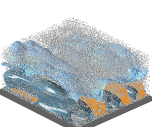
Figure 7 displays an enlarged view of the vorticity and particle distribution ( $St=53$) near the TNTI in the $z$–
$z$– $y$ plane, corresponding to the $x-$position indicated by the white dashed line in figure 5(d). In this figure, the black arrows indicate the velocity vectors of the particles and the red bold arrow near the vortex core denotes its direction of rotation. It can be found that, due to the centrifugal effect, the particles are mainly distributed at the edge of the large-scale vortical structures (high tangential velocity) in the turbulent region where they move at higher speed.

Figure 7. Instantaneous vorticity and particle distributions for  $St=53$.
Since the magnitude of the vertical velocity of the particles is directly related to the transport of particles across the TNTI, we further show in figure 8 the conditionally averaged particle vertical velocity  $\langle v_{p}\rangle$ near the TNTI. It shows that $\langle v_{p}\rangle >0$ within the turbulent region below the TNTI and $\langle v_{p}\rangle <0$ in the non-turbulent region, which indicates that the particles on both the turbulent and non-turbulent sides away from the TNTI tend to move towards the TNTI. In the potential flow region, the small mean vertical velocity of particles might be ascribed to the swallowing (the entrainment process that irrotational pockets of fluid are swallowed into the TBL) of the TNTI (Mathew & Basu Reference Mathew and Basu2002; Reuther & Kähler Reference Reuther and Kähler2018). Whereas, on the turbulent side, the high-speed vertical transport of centrifuged particles towards the TNTI is blocked by the potential flow (irrotational), preventing them from further upward transport. Therefore, a significant accumulation zone below the TNTI ( $-0.1<\zeta / \delta <0$) is formed for the highest-inertia particles studied. Elsinga & Da Silva (Reference Elsinga and Da Silva2019) reported a similar blocking effect by analysing the average velocity and scalar fields in planar turbulent jets and shear-free turbulence in the strain eigenframe. One may also speculate why the particles cluster at the TNTI with the notion of turbophoresis, that is, there should be a drift of particles from higher turbulence intensity (within the turbulent part of the boundary layer) to lower turbulence intensity (outside the TBL). We present in figure 8 the turbophoresis velocity $v_{t u r}=-\tau _{p} \partial < v^{\prime 2}>/ \partial y$ (the dashed lines). It is seen that $v_{t u r}>0$ near the TNTI. Particles, especially those with large inertia, may break through the interface only under the act of turbophoresis, which is contradictory to the accumulation phenomenon. Although the turbophoresis does play a role in transporting particles upward, it is not the main reason for particle accumulation beneath the interface.

Figure 8. Conditionally averaged vertical velocity of particles.
3.3. Statistics of the fluid near the TNTI
The conditionally averaged streamwise fluid velocities  $\langle u_{f}\rangle$ are shown in figure 9(a). First, $\langle u_{f}\rangle$ significantly changes near the TNTI for particle-free TBL. However, the well-defined sharp jump (the slope of the curve is required to be steeper somewhere along its range near the TNTI) across the TNTI reported in particle-free flows (Chauhan et al. Reference Chauhan, Philip and Marusic2014a; Eisma et al. Reference Eisma, Westerweel, Ooms and Elsinga2015) cannot be observed from the $\langle u_{f}\rangle$ profiles in figure 9(a). By checking the data and the employed methods, we find that the disappearing jump in $\langle u_{f}\rangle$ is attributed to the identification method of the TNTI. We can observe the velocity jumps near the TNTI when the kinetic energy threshold is employed. Most importantly, $\langle u_{f}\rangle$ in the particle-laden TBL is smaller than that in particle-free TBL. The reduced conditionally averaged velocities are the result of the decreased mean height of the TNTI. In the particle-laden TBL, the interface will see a flow slower than that in the particle-free TBL since it is closer to the wall, as shown in figure 4. These are more pronounced as the particle Stokes number increases. Further, the more obvious change in $\langle u_{f}\rangle$ for the particle-laden TBL with high-inertia particles also implies a larger velocity gradient.

Figure 9. Conditionally averaged (a) mean streamwise velocity and (b) vorticity for particle-free and particle-laden flows.
Turning now to the vorticity near the TNTI. Figure 9(b) illustrates the conditionally averaged vorticity  $\langle \omega ^{*}\rangle$. Previous studies have observed a vorticity jump across the TNTI, regardless of the Reynolds number, the identification method of the TNTI and the definition of the TNTI coordinate (Chauhan et al. Reference Chauhan, Philip, de Silva, Hutchins and Marusic2014b; Borrell & Jiménez Reference Borrell and Jiménez2016; Long et al. Reference Long, Wu and Wang2021; Zhang et al. Reference Zhang, Watanabe and Nagata2023). The vorticity jump is also observed in particle-free TBL in this study, although it was not significant (shown later). In particle-laden flows, $\langle \omega ^{*}\rangle$ is larger than that in particle-free flow. This is also more significant with an increase in the particle inertia. Meanwhile, the presence of particles may lead to a more significant jump of the mean vorticity than in particle-free flow. This is particularly clear for $St=53$. The slope of the $\langle \omega ^{*}\rangle$- $\zeta /\delta$ curve increases rapidly near the interface and reaches a maximum near the particle accumulation region, indicating a direct relation between the degree of particle accumulation and the vorticity jump.
The TNTI layer is an instantaneous region between the turbulent field and the non-turbulent fluid. Within this region, the transport of vorticity is very important to understand the TNTI. We show the conditional enstrophy budgets for all the simulation cases in figure 10. By applying the curl operator to (2.2) and then multiplying it by the vorticity vector  $\boldsymbol {\omega }$, the enstrophy ( $\varOmega \equiv \boldsymbol {\omega } \boldsymbol{\cdot} \boldsymbol {\omega }$) equation including the particle feedback force can be obtained
 \begin{equation} \underbrace{\frac{{\rm D} \varOmega}{{\rm D} t}}_{T_{\varOmega}}=\underbrace{2 \boldsymbol{\omega} \boldsymbol{\cdot}(\boldsymbol{\omega} \boldsymbol{\cdot} \boldsymbol{\nabla} \boldsymbol{u})}_{P_{\varOmega}}+\underbrace{v \nabla^{2} \varOmega}_{D_{\varOmega}}-\underbrace{2 v \boldsymbol{\nabla} \boldsymbol{\omega}: \boldsymbol{\nabla} \boldsymbol{\omega}}_{E_{\varOmega}}+\underbrace{2 \boldsymbol{\omega} \boldsymbol{\cdot}(\boldsymbol{\nabla} \times \boldsymbol{f})}_{F_{\varOmega}}. \end{equation}
Figure 10. Conditionally averaged enstrophy budgets for all the simulations; (a) enstrophy production, (b) enstrophy diffusion, (c) enstrophy dissipation terms and (d) the contribution of the particle feedback force  $\langle F_{\varOmega }\rangle$ to the enstrophy for particle-free flow and particle-laden flows.
The terms in (3.1) represent in turn the total variation of enstrophy ( $T_{\varOmega }$), the enstrophy production ( $P_{\varOmega }$), the viscous diffusion ( $D_{\varOmega }$), the viscous dissipation ( $E_{\varOmega }$) and the contribution of the particle feedback force ( $F_{\varOmega }$). Here, all terms are normalized by $(U_{\infty } / \theta _{i n})^{3}$. All the enstrophy governing terms are virtually zero in the non-turbulent region for both particle-free and particle-laden flows. Deep inside the turbulent region the enstrophy production and viscous dissipation roughly balance in particle-free flow. Viscous diffusion acts to migrate vorticity from the boundary layer into the outer irrotational region (Jahanbakhshi Reference Jahanbakhshi2021) and is positive in the region very close to the TNTI. It never overtakes any of the other enstrophy equation terms, except for in the region near the TNTI. The enstrophy production and viscous dissipation in particle-laden flow are larger in magnitude than those in particle-free flow. The increase is likely because the presence of particles makes the TNTI closer to the high-vorticity region, where the strain is higher. In particle-laden flow $\langle E_{\varOmega }\rangle$ is always larger than $\langle P_{\varOmega }\rangle$ in magnitude, implying that the small-scale eddies increase near the interface since dissipation mainly occurs at small scales. Here, $\langle D_{\varOmega }\rangle$ increases and shifts towards the interface due to the accumulation of the particles. In addition, $\langle F_{\varOmega }\rangle >0$ below the TNTI for all cases and $\langle F_{\varOmega }\rangle$ is almost the same as $\langle P_{\varOmega }\rangle$ for $St=53$. It behaves as the production term in the enstrophy equation. The sum of $\langle F_{\varOmega }\rangle$, $\langle P_{\varOmega }\rangle$ and $\langle D_{\varOmega }\rangle$ is larger than $|\langle E_{\varOmega }\rangle |$ near the TNTI, which explains why the conditionally averaged vorticity increases in the turbulent region (figure 9b). It can also be observed that, in the range of $-0.1<{\zeta }/{\delta }< 0$, the contribution of the particle feedback force to the vorticity decreases sharply with $\zeta / \delta$, corresponding to the observed vorticity jump. These phenomena are more pronounced at high Stokes number ( $St=53$).
Finally, we present the premultiplied one-dimensional  $u-$spectra ( $K_{z} E_{u u} / u_{\tau }^{2}$) (which can show the integral contribution per $K_{z}$) as a function of spanwise wavelength $\lambda _{z}$ and wall-normal distance to the TNTI ( $y-y_{i}$) in figure 11 for particle-laden flow with $St=53$, particle-free flow and their difference. Here, $K_{z}$ and $\lambda _{z}$ denote the spanwise wavenumber and wavelength. In this coordinate system, the streamwise fluctuating velocity is $u^{''}=u-u^{*}$, where $u^{*}$ is the conditionally averaged velocity based on $y-y_{i}$. Then $u^{''}$ is used to obtain $E_{u u}$ in figure 11. Only the results for $(y-y_{i}) / \theta _{i n}\leq 0$ are shown because flow in the region of $(y-y_{i}) / \theta _{i n}>0$ is non-turbulent. It can be seen that the energy spectra are augmented for all turbulent wavenumbers due to the addition of inertial particles. The increase is more pronounced in the low wavenumber range ( $\log _{10} \lambda _{z}^{+} \approx 2.5 \text { or } \lambda _{z} \approx 0.65 \delta$), which might be attributed to the interaction between the particles and large-scale eddies in the outer region of the TBL seen by the TNTI. It has been accepted that the TNTI is generated by vorticity structures in the nearby turbulent region (da Silva, dos Reis & Pereira Reference da Silva, dos Reis and Pereira2011). Lee et al. (Reference Lee, Sung and Zaki2017) found that the large-scale motions modulate the TNTI height. Therefore, the particles will indirectly change the TNTI properties by modifying the large-scale turbulent structures in the turbulent boundary layer.

Figure 11. Premultiplied one-dimensional  $u$-spectra as functions of spanwise wavelength $\lambda _{z}$ and distance to the TNTI in the wall-normal direction $y-y_{i}$. Panel (a) is for particle-laden flow with $St=53$. Panel (b) is for particle-free flow. Panel (c) is the difference between (a,b).
3.4. Effects of particles on the geometric properties of the TNTI
Based on the above analysis of the flow fields near the TNTI, it is supposed that the presence of particles may affect the features of the TNTI because of their two-way coupling. This section aims to analyse the p.d.f. of the height, the fractal dimension, the entrainment velocity of the TNTI and the thickness of the TNTI layer.
Figure 12 shows the top view of the vorticity iso-surfaces (the TNTI), which is obtained using the selected vorticity magnitude threshold and is coloured by the instantaneous (local) values of the TNTI height for all the simulations carried out in this study. For the particle-free flow shown in figure 12(a), the most prominent characteristics are the streamwise-aligned structures that modulate the TNTI into bulges and valleys, as well as the small-scale wrinkles sitting on large-scale indentations. This is similar to the observation in Jahanbakhshi (Reference Jahanbakhshi2021) at similar Reynolds numbers. These small-scale wrinkles resemble trains of hairpin vortices that are typical in wall-bounded turbulence (Chauhan et al. Reference Chauhan, Philip, de Silva, Hutchins and Marusic2014b). With the addition of low- and moderate-inertia particles, the shape of the TNTI shows less apparent changes, as seen in figure 12(b,c). However, a clear difference from the particle-free flow can be visibly observed for case  $St=53$. The wrinkles on the large-scale indentations of the TNTI in particle-laden TBL become less pronounced. There is a decreasing tendency in the complexity of the TNTI. Next, we will discuss the geometric characteristics of the interface starting from the distribution of interface height and fractal dimension of the TNTI.

Figure 12. Top view of the iso-surfaces obtained by applying the selected vorticity magnitude threshold for particle-free flow (a) and particle-laden flow with  $St=2$ (b), $St=11$ (c), $St=53$ (d).
The variation of the TNTI height represents the spatial undulation of the TNTI. Figure 13(a) shows the p.d.f.s of the TNTI height  $y_{i}$, with the horizontal coordinates being non-dimensionalized in terms of the respective mean height of the TNTI $\delta _i$. Previous studies believed (Gampert et al. Reference Gampert, Boschung, Hennig and Gauding2014; Balamurugan et al. Reference Balamurugan, Rodda, Philip and Mandal2020) or assumed (Wu et al. Reference Wu, Wang, Cui and Pan2020) that the p.d.f. of the TNTI height is Gaussian. However, the experimental work of Wu et al. (Reference Wu, Wang, Cui and Pan2020) reported a non-Gaussian function of $y_i$ on different directional riblet surfaces at different Reynolds numbers $(Re_{\tau }= 382, 548, 680, 820)$; $y_i$ shows a positive skewness for the converging riblet surface while a negative skewness for the diverging riblet surface. We observe non-Gaussian distributions of $y_i$ in both particle-free and particle-laden TBLs. Figure 13(a) indicates that the p.d.f. of $y_i$ is positively skewed, analogously to the experimental results of Wu et al. (Reference Wu, Wang, Cui and Pan2020) on the converging riblet surface. Moreover, the variances $\sigma _{y_{i}}$ of $y_{i}$ in particle-laden flow are much higher ( $\sigma _{y_{i}}=3.8$ for $St = 2$, $\sigma _{y_{i}}=4.0$ for $St = 11$ and $\sigma _{y_{i}}=4.5$ for $St = 5$3) than that in particle-free flow ( $\sigma _{y_{i}}=3.7$).

Figure 13. (a) The p.d.f. of the TNTI height. (b) The fractal dimension of different interfaces.
The fractal dimension of the TNTI is a statistical measure of its complexity and indicates how contorted it is. It is commonly used to assess the characteristics of the TNTI (e.g. Sreenivasan et al. Reference Sreenivasan, Ramshankar and Meneveau1989; Borrell & Jiménez Reference Borrell and Jiménez2016). For a smooth three-dimensional surface, the fractal dimension is  $D_{f}=2$. A common method used to calculate the fractal dimension is the box-counting method (Chauhan et al. Reference Chauhan, Philip and Marusic2014a; Borrell & Jiménez Reference Borrell and Jiménez2016; Wu et al. Reference Wu, Wang, Cui and Pan2020). In this method, the flow field involving the TNTI is divided into square boxes of a certain size ( $b / \delta$). The number of boxes $N$ required to cover the instantaneous TNTI is recorded. Theoretically, if $N \sim (b / \delta )^{D_{f}}$, then $D_{f}$ is defined as the fractal dimension. Also, $D_{f}$ can be determined by the slope of the $N \sim (b / \delta )$ plot in log–log coordinates. We plot the average box number $N$ as a function of box size $b / \delta$ in figure 13(b) according to the results from $200$ instantaneous flow fields, in which the horizontal and vertical coordinates are shown in logarithms. For each case, a linear fit is performed for the scattered data points and the slope of the line represents the fractal dimension $D_{f}$. The $D_{f}$ values for the four cases are displayed in the inset of figure 13(b).
Sreenivasan et al. (Reference Sreenivasan, Ramshankar and Meneveau1989) argued that the fractal dimension is  $D_{f} \approx 2.36$ in the TBL and shear flow. de Silva et al. (Reference de Silva, Philip, Chauhan, Meneveau and Marusic2013) found $D_{f} \approx 2.3\unicode{x2013}2.4$ in more recent TBL experiments. Wu, Zaki & Meneveau (Reference Wu, Zaki and Meneveau2019) showed that turbulent spots have a fractal dimension of $D_{f} \approx 2.36$ during the transition from laminar to turbulent flow. Wu et al. (Reference Wu, Wang, Cui and Pan2020) concluded that $D_{f} \approx 2.2$ for the TBL, and the diverging and converging riblet surfaces do not substantially affect the fractal dimension of the TNTI. Recently, Zhang et al. (Reference Zhang, Watanabe and Nagata2023) found that the fractal dimension $D_{f}$ is $2.14-2.20$ in temporally developing TBLs. An increase in the Reynolds number may result in an increase in the fractal dimension of the TNTI, but $D_{f}$ does not increase monotonically at relatively low Reynolds numbers. Our simulations show $D_{f}=2.31$ in particle-free flow within the range of $2\eta _{I}< b<0.4\delta$, which is very close to the values previous studies reported. The presence of particles affects the fractal dimension of the TNTI ( $D_{f}=2.29$ for $St=2$, $2.25$ for $St=11$ and $2.14$ for $St=53$), indicating a reduced complexity of the TNTI as particle inertia increases. It is worth noting that Borrell & Jiménez (Reference Borrell and Jiménez2016), in particle-free flow, found that as the vorticity threshold ( $\omega ^*_{th}$) increases, the geometric complexity and fractal dimension of the identified TNTI increases. The results in this study show that the fractal dimension of the TNTI decreases with the increase of the Stokes number despite, conversely, $\omega ^*_{th}$ increasing (figure 4). This further indicates the distinctive modulation effect of particles on the TNTI.
Lee et al. (Reference Lee, Sung and Zaki2017) found that the high- and low-speed LSMs correspond to the spatial undulations of the TNTI, where the crest in the shape of the TNTI is associated with the high-speed LSM and the trough is associated with the low-speed LSM. According to the energy spectrum shown in figure 11, we know that the presence of particles changes the large-scale turbulent structures in the turbulent region the TNTI sees. In order to further investigate the effect, the method proposed by Nolan & Zaki (Reference Nolan and Zaki2013) is deployed to extract the LSMs. The method is simply specified as follows. First, we calculate the spanwise two-point correlation  $R_{u^{\prime } u^{\prime }}(\Delta z)$ of the streamwise fluctuating velocity $u^{\prime }$. The correlation size corresponding to $R_{u^{\prime } u^{\prime }}(\Delta z)=0.5$ is selected to filter the flow field. The small-scale turbulence is hence eliminated by Gaussian filtering to obtain the filtered perturbation field $\hat {u}$. Then, we search the local extrema of $\hat {u}$ in terms of $\partial \hat {u} / \partial y=\partial \hat {u} / \partial z=0$. The cores of the LSMs are identified using the local extrema of $\hat {u}$ and its connectivity in the streamwise direction. Finally, the iso-surface with the threshold of $0.1 U_{\infty }$ is used to identify the high-speed ( $\hat {u}>0.1 U_{\infty }$) and low-speed ( $\hat {u}<-0.1 U_{\infty }$) coherent structures. This method was also employed by Lee et al. (Reference Lee, Sung and Zaki2017) to extract the cores of the LSMs for high- and low-speed structures and analyse their relationships with the near-TNTI turbulent statistics and dynamics.
Figure 14 displays the conditionally averaged velocity fields based on the core of high- and low-speed LSMs at  ${y}_{{ref }}=0.25 \delta _{99}$ in the $x$–
$x$– $y$ plane for the four simulations, in which the abscissa is the streamwise distance from the cores of the LSMs and the small black solid rectangles indicate the conditionally averaged height of the TNTI corresponding to the LSMs (the value of the height is shown in each panel). The top-row panels show the conditionally averaged high-speed large-scale structures and the bottom-row panels show the low-speed large-scale structures. We emphasize that the ordinate in these figures is the distance from the bottom wall. It is seen from figure 14(a i,ii) that the height of the TNTI corresponding to the high-speed LSM ( $y_i$=0.998 $\delta$) is lower than that to the low-speed LSM ( $y_i=1.012\delta$), which is consistent with Lee et al. (Reference Lee, Sung and Zaki2017), and this relationship persists in particle-laden flow. The corresponding TNTI heights for both high- and low-speed structures in particle-laden flow are lower than those in particle-free flow and the reduction becomes more significant for increasing Stokes numbers and the high-speed LSMs. Since particles tend to cluster at the outer margin (high-speed region) of the large-scale eddies in the turbulent region, as indicated in figure 7, they will interact more strongly with high-speed flow. Accordingly, the difference $\Delta y_{i}$ between the mean values of the TNTI height corresponding to the high- and low-speed structures is apparently increased in particle-laden TBL. For instance, $\Delta y_{i}=0.014 \delta$ for particle-free flow and $\Delta y_{i}=0.12 \delta$ for case $St=53$, implying that the presence of particles results in an increase in the undulation of the TNTI, which is an important reason for the increase in the variance of the p.d.f. of the TNTI height in figure 13(a). Most significantly, the shape of the large-scale structure in particle-laden flow significantly differs from that in the particle-free case. The larger the particle Stokes number is, the smoother the velocity correlation structure becomes and its inclination angle from the wall decreases, thus making the fractal dimension of the TNTI decrease.

Figure 14. Conditionally averaged velocity fields based on the core of (i) high- and (ii) low-speed LSMs at  $y_{{ref }}=0.25\delta _{99}$; (a) particle-free flow, (b) particle-laden flow with $St=2$, (c) $St=11$, (d) $St=53$. The flood contour is the conditionally streamwise velocity fluctuation $u^\prime$. The black dashed lines indicate the contour line of $u^\prime$= $\pm 0.02U_\infty$.
According to Jahanbakhshi (Reference Jahanbakhshi2021), the changes in the shape of the TNTI can be quantitatively described by the entrainment velocity  $V_{Total}$, which is expressed as
 \begin{equation} V_ {Total }=\frac{1}{|\boldsymbol{\nabla} \varOmega|} \frac{\mathrm{D}\varOmega}{\mathrm{D} t}=\frac{T_{\varOmega}}{|\boldsymbol{\nabla} \varOmega|} .\end{equation}
The positive value of  $V_{Total}$ indicates an increase in enstrophy, which means that the TNTI is moving in the direction toward the non-turbulent region. If the fluid in non-turbulent region moves toward the turbulent region with $V_{Total}<0$, it leads to a transition from turbulent to non-turbulent flow. In particle-free flow, the positive values of $V_{Total}$ are predominantly associated with the crests of the TNTI, whereas negative values are linked to the troughs (Abreu et al. Reference Abreu, Pinho and da Silva2022). The entrainment encompasses two mechanisms, one is referred to as small-scale nibbling while the other, related to large-scale eddies, is called engulfment. The nibbling-type entrainment is believed to be caused by the outward spreading of vorticity due to viscosity in the proximity of the TNTI layer and hence contributes more positive entrainment velocities, while the engulfment-type entrainment is achieved by digestion of large-scale pockets of non-turbulent fluids into the turbulent core before acquiring vorticity if the interface is intensely folded. Therefore, the change in the total entrainment velocity is essentially a manifestation of the change in turbulent structures of different scales.
Figure 15(a) depicts the p.d.f.s of  $V_{Total}$ at the TNTI ( $\zeta / \delta =0$) in particle-free flow and particle-laden flow and figure 15(b) shows the values of the peak, the mean, the skewness and the kurtosis of these p.d.f.s. It can be seen that the peak of the p.d.f. is positive for particle-free flow, which is consistent with Jahanbakhshi (Reference Jahanbakhshi2021) and Zhang et al. (Reference Zhang, Watanabe and Nagata2023). This indicates that the interface more frequently propagates to the non-turbulent region. Accordingly, the mean $V_{Total}$ is higher than zero, indicating that the small-scale nibbling has a prevalent influence on the entrainment. The skewness is toward the negative side. This is in agreement with Jahanbakhshi (Reference Jahanbakhshi2021) but in contrast to Zhang et al. (Reference Zhang, Watanabe and Nagata2023), which might be explained by the dependence of the p.d.f. on the Reynolds number. Actually, Zhang et al. (Reference Zhang, Watanabe and Nagata2023) have revealed that the p.d.f. of $V_{Total}$ for ${Re}_\theta >4000$ is different from ${Re}_\theta <2000$. In particle-laden flow, the p.d.f.s of the entrainment velocity become boarder, corresponding to the wider distribution of the TNTI height. It is relevant to the bigger sized large-scale eddies in particle-laden TBL, as shown in figure 14, since the bigger eddies will result in bigger tangential velocities on their periphery (Abreu et al. Reference Abreu, Pinho and da Silva2022). The positive peaks of the $V_{Total}$ p.d.f.s in particle-laden flow increase partly because the large-scale structures in the turbulent region modulating the TNTI become flatter, less inclined and hence the interface is moderately folded (the probability of $V_{Total}<0$ decreases). Meanwhile, the enhanced enstrophy diffusion (figure 14b) gives rise to augmented outward spreading of vorticity ( $V_{Total}>0$). By the same token, the negative bias is evidently reduced by the presence of particles although $V_{Total}$ still has a negative skewness distribution. Furthermore, the kurtosis of the p.d.f. in particle-laden flow is much smaller than that in particle-free flow, implying a decrease in the ‘roughness’ of the TNTI, which further explains the decrease in the fractal dimension.

Figure 15. (a) Probability density functions of the entrainment velocity  $V_{Total}$ on the TNTI. (b) The peak, the mean, the skewness and the kurtosis of these p.d.f.s.
The thickness of the TNTI layer can be quantified based on the derivative of the vorticity magnitude since this layer is a region with a strong vorticity gradient that adjusts the vorticity magnitude between turbulent and non-turbulent regions (Zhang et al. Reference Zhang, Watanabe and Nagata2018). Here, the thickness is determined by measuring the distance from the TNTI to the location where the vorticity gradient is flat. We calculate the gradient of vorticity  $d<\omega ^*>/d\zeta$ near the TNTI and show the results in figure 16(a). Since the TNTI changes most significantly for the high-inertia case, only the results for $St=53$ are shown and compared with the particle-free flow. As seen in figure 16(a), $d<\omega ^*>/d\zeta$ decreases rapidly on the turbulent side after experiencing a peak near the interface. The thickness of the TNTI layer in the particle-free flow is approximately $0.2\delta$ ( $15.6\eta _{I}$) if we choose a small threshold of $d^2<\omega ^*>/d\zeta ^2=0.008$. This is consistent with previous observations of ${\sim }O(10\eta _{I})$ (Zhang et al. Reference Zhang, Watanabe and Nagata2018; Long et al. Reference Long, Wang and Pan2022). However, with the same threshold of $d^2<\omega ^*>/d\zeta ^2$, the TNTI layer thickness is just $0.15\delta$ ( $11.7\eta _{I}$) for the TBL laden with high-inertia particles, reduced by $25\,\%$, implying that the presence of particles compresses the TNTI layer. This may be ascribed to the particle accumulation just beneath the TNTI, which will limit the free development of the interface layer through two-phase interactions. Further, the viscous diffusion and the generation term in the enstrophy equation are depicted in figure 16(b) to discern the two sublayers of the TNTI layer, the VSL and the TSL. In the VSL, the viscous diffusion dominates $\langle D_{\varOmega }\rangle >\langle P_{\varOmega }\rangle$, while in the TSL, the generation term generated by vortex stretching dominates and $\langle P_{\varOmega }\rangle >\langle D_{\varOmega }\rangle$. Abreu et al. (Reference Abreu, Pinho and da Silva2022) determined the thickness of the two sublayers through the intersection of $\langle P_{\varOmega }\rangle$ and $\langle D_{\varOmega }\rangle$. It can be observed that the VSL thickness for the particle-free flow is $0.05\delta$ ( $3.90\eta _{I}$), which is consistent with that reported in Long et al. (Reference Long, Wang and Pan2022). However, it reduces to $0.024\delta$ ( $1.88\eta _{I}$) in the particle-laden case, approximately reduced by $52\,\%$ as compared with the particle-free TBL. The presence of particles compresses the VSL thickness more significantly. This could be expected because the accumulation of particles (the conditionally averaged particle volume fraction for St =53 is also depicted) beneath the interface makes the curve of the viscous diffusion shift upward. Subsequently, the intersection point of the $\langle P_{\varOmega }\rangle$ and $\langle D_{\varOmega }\rangle$ profiles moves up too.

Figure 16. (a) Conditional mean profiles of the vorticity derivative with respective to  $\zeta$ for particle-free flow and particle-laden flow with $St=53$. (b) Conditionally averaged enstrophy as well as enstrophy production and diffusion for particle-free flow and particle-laden flow with $St=53$. The blue dash-dot line indicates conditionally averaged particle volume fraction $C_v$ for particle-laden flow with $St=53$.
Finally, the explanation of the thinner TNTI layer has to do with the fact that the vorticity jump is caused by the intense vorticity structures alongside the TNTI (da Silva & Taveira Reference da Silva and Taveira2010), which themselves play a crucial role in shaping the TNTI and determining the thickness of the TNTI layer (Taveira & da Silva Reference Taveira and da Silva2014; Abreu et al. Reference Abreu, Pinho and da Silva2022). Silva, Zecchetto & da Silva (Reference Silva, Zecchetto and da Silva2018) found that a more fragmented vortex implies a decrease in the average thickness of the TNTI in shear-free turbulence and temporal turbulent planar jets. The top view of the vortex structures near the TNTI is presented in figure 17 for both particle-free flow and particle-laden flow with  $St=53$. These structures are identified by the iso-surfaces of the second invariant of the velocity gradient tensor $Q$ (Hunt, Wray & Moin Reference Hunt, Wray and Moin1988). Here, $Q$ is defined as $Q=(\omega _{i j}\omega _{i j}-S_{i j}S_{i j})/2$, with $\omega _{i j}=(\partial u_{i} / \partial x_{j}-\partial u_{j} / \partial x_{i}) / 2$ and $S_{i j}=(\partial u_{j} / \partial x_{i}+\partial u_{i} / \partial x_{j}) / 2$. It can be found that, in both cases, the TNTI layer is filled with vortex structures. However, for the particle-laden case, these vortex structures differ in shape and number from the particle-free flow. The presence of particles makes the vortex structures near the TNTI more fragmented, smaller in scale and more irregular in shape. Accordingly, the TNTI layer becomes thinner.

Figure 17. Iso-surfaces of the second invariant of the velocity gradient tensor  $Q$, corresponding to a threshold of $Q=3 \times 10^{-5}$, (a) particle-free flow, (b) particle-laden flow with $St=53$.
4. Conclusions
Direct numerical simulations of a spatially developing flat-plate boundary layer  $(R e_{\theta }= 300\unicode{x2013}1210)$ free from and laden with inertial particles ( $St=2$, $11$ and $53$) are performed to investigate the properties of the TNTI. For the particle-laden case, the two-way coupled Eulerian–Lagrangian point-particle approach is employed. The simulation is validated by previous studies on particle-free and particle-laden TBLs. It seems to be the first study addressing the effect of inertial particles on the TNTI despite there being much research focusing on particle–turbulence interaction in the inner and outer layers of wall turbulence.
The TNTI is detected by vorticity magnitude and validated by the turbulent volume fraction criterion, described and used in numerous works. The addition of inertial particles is found to increase the vorticity magnitude threshold for the TNTI identification and decreases the mean height of the TNTI as compared with the unladen case. In terms of the conditional sampling based on the local coordinates of the TNTI, we find that particles may accumulate in the region just beneath the TNTI, mainly due to the centrifugal effect of the large-scale vortical structures on the turbulent side of the TNTI and the barrier effect of the potential flow, as well as the swallowing effect of particles in the non-turbulent region by the TNTI. This phenomenon is more pronounced as particle inertia (measured by the Stokes number) increases.
The accumulation of particles significantly reduces the conditionally averaged fluid velocity and increases the velocity gradient below the interface. The latter variation is also accompanied by a much clearer jump in the mean vorticity across the TNTI in particle-laden flow than in particle-free flow, resulting in a thinner TNTI layer. By analysing the enstrophy equation, it is revealed that inertial particles provide a positive feedback to the enstrophy equation below the TNTI. Consequently, the production, viscous dissipation and viscous diffusion terms are all increased in magnitude in particle-laden turbulence, explaining why the conditionally averaged vorticity increases in the turbulent region as compared with the unladen TBL. Meanwhile, the viscous diffusion terms shift towards the interface due to the accumulation of the particles. As a result, the intersection point of production and viscous diffusion curves moves toward the interface, implying a reduced viscous sublayer of the TNTI layer.
Moreover, the addition of inertial particles will give rise to a bigger undulation (higher variances of the TNTI height) and less complexity (smaller fractal dimension) of the TNTI. The underlying physics is revealed by looking at eddies in the turbulent region, as well as the entrainment velocity on the interface. The energy spectrum of the streamwise fluctuating velocity seen by the interface is augmented for all turbulent wavenumbers due to the addition of inertial particles. The augmentation is more pronounced in the low wavenumber range, indicating a clear change in large-scale structures in the outer layer of the TBL since the shape of the TNTI is strongly correlated with these structures. Results confirm that the extracted high- and low-speed LSMs are apparently changed by particles. The LSMs becomes larger in size, smoother and less inclined. Accordingly, the p.d.f.s of the entrainment velocity become boarder and the kurtosis of the  $V_{Total}$-p.d.f. decreases. Therefore, the interface in particle-laden TBL is more undulated and its ‘roughness’ decreases, which further explains the decrease in the fractal dimension. Just beneath the interface, the vortex structures become more fragmented because of the influence of particle accumulation. This is the direct reason for a thinner TNTI layer.
We study two-phase interactions at three Stokes numbers (by varying the density ratio), with a relatively moderate level of inertia, and report the Stokes number dependence of the features of the TNTI. Future research should focus on the behaviour of higher-inertia particles and examine the effects of varying mass fractions, taking the gravitational settling and particle collisions into account. In addition, a wider range of Reynolds numbers, for example  ${Re}_\theta =3000$, is necessary to better represent an equilibrium TBL.
Acknowledgements
We thank the three anonymous referees for their useful comments.
Funding
X.J.Z. and Q.Q.W. are supported by National Natural Science Foundation of China (grant number 12388101 and grant number 92052202). P.W. is supported by National Natural Science Foundation of China (grant number 12072138), the National Key Scientific and Technological Infrastructure project ‘Earth System Numerical Simulation Facility’ (EarthLab) and Natural Science Foundation of Gansu Province (no. 23JRRA1035).
Declaration of interests
The authors report no conflict of interest.


