


1. Introduction
The foundry process converts liquid metal into the desired shape, that is., metal casting [Reference Hazela, Hymavathi, Kumar, Kavitha, Deepa, Lalar and Karunakaran1]. At present, the pouring task of large castings still relies mainly on manual participation. But, there are numerous major issues with foundry production today, including hostile environments, overcapacity, manual labor demands, high labor intensity, and frequent personnel turnover. The intelligence level of foundry firms in China is now varied [Reference Gong, Hu, Liu, Yang, Jiang and Fan2]–[Reference Sithole, Nyembwe and Olubambi4]. These problems seriously constrain the improvement of casting intelligence level. Sand mold casting is dependent on the iron pouring process, which directly affects the final quality of the castings. About the earlier research on pouring robots, foreign researchers mainly studied its control methods by designing a simple mechanical system model. Terashima et al. designed an inclined automatic pouring machine and proposed a two-degrees-of-freedom (DOF) control system that could keep a constant liquid level of a sprue cup [Reference Kazuhiko, Ken’ichi and Yu5]. Yoshiyuki et al. developed a cylindrical ladle automatic-conveying pouring machine that realized the suppression of shaking [Reference Noda, Terashima, Suzuki and Makino6]. And also proposed a ladle effluent drop position monitoring system [Reference Noda, Fukushima and Terashima7]. The pouring process involves high-temperature liquid metal, and these semi-automated pouring systems, which require manual assistance, lack safety and reliability and are gradually becoming unsuitable for the needs of the new era.
With the development of robotics in smart manufacturing, it is gradually being applied to traditional casting processes. Pan Guangtang designed an industrial robot aluminum alloy large piston casting system by optimizing the piston casting production process [Reference Guangtang8]. Li et al. designed an automatic monitoring system for the tilting hydraulic pouring machine, which can realize 6-level tilting speed conversion [Reference Haibo, Xinxing and Jinyu9]. The fully automatic pouring equipment developed and designed by Zhou et al. can realize automatic pouring without backflow following the ingot casting machine [Reference Pu, Xuejie and Yong10]. Regrettably, there is no existing literature on heavy-duty casting of large parts, which is the focus of our research. Because the hybrid robot has the advantages of large working space, strong load capacity, good dynamic performance, and high motion accuracy [Reference Guo, Cheng, Wang and Li11]. Therefore, in order to realize heavy-duty pouring tasks at different stations, the design method of hybrid mobile robot arm is adopted instead of the traditional articulated robot arm. For instance, Li et al. designed the hybrid truss heavy-load pouring robot and proposed a Newton-Euler iterative estimation method to realize ladle attitude control [Reference Long, Chengjun, Yongcun and Hongtao12]–[Reference Li, Wang, Gu and Wu14]. While this factory overhead crane-like lifting method allows for heavy-duty pouring, the top-down working arm allows for limited spatial flexibility and reduced robot tipping capability.
In addition, the theoretical studies on the control of the end ladle casting process mainly include the following: liquid-level monitoring, ladle-level detection, pouring liquid quality measurement, flow rate and angle estimation, etc. ways to realize intelligent pouring. In addition, the pouring task is a complex serialized process, and it is difficult to establish a fixed model for different pouring tasks [Reference Wang, Tian and Pan15]. Takaaki et al. combined the flow nonlinear feedforward tracking control with linear PID feedback design model controller to obtain more accurate robust racking performance and stability [Reference Tsuji and Noda16]. Conventional control strategies do not accurately model the casting control process [Reference Do, Gordillo and Burgard17]. Therefore, it is a challenge for the robot to accurately pour to the sprue port on the sandbox in different scenarios. In addition, the irreversible feature of the pouring task [Reference Huang, Wilches and Sun18]. A portion of the pouring liquid from a single pour is retained between the pouring nozzle and the pouring spout.
In contrast, deep learning-based control algorithms have been widely adopted in various robotics applications due to their higher accuracy and faster speed, which can effectively improve the control accuracy and fast model prediction [Reference Zhao, Xie, Miao and Xia19]–[Reference Yang, Zhang and Sudjianto20]. Tianze et al. adopted recurrent neural networks to do the experiment of the dynamic model predictive control of the water and obtained the optimal speed for precise dumping [Reference Soufiani and Adlı22]. Huang et al. [Reference Huang, Wilches and Sun18] utilized a self-supervised learning demonstration method based on long-short-term memory to make robot pour accurately and quickly like human beings. Babak et al. used pole placement and linear quadratic regulator control technique to achieve high-speed wobble-free delivery of liquid-filled containers by linearizing the nonlinear liquid agitation dynamics [Reference Ryosuke, Junsuke and Kazuki23]. The control system has a longer run time and lacks in angular size control. Furthermore, none of them use visual information. Control based on visual feedback allows more information to be obtained and is therefore adopted by us. On the research of estimation methods based on the combination of depth vision and volume, Tasaki Ryosuke [Reference Kennedy, Schmeckpeper and Thakur24], Monroe Kennedy [Reference Zhu and Yamakawa25], Zhu HR [Reference Chau and Wolfram26], and others have done related work respectively. However, task-based optimization is needed to determine the appropriate parameters for the best performance. In the research based on the combination of depth vision and liquid level, Do Chau [Reference Defang, Chencong and Zhenxia27], Cheng DF [Reference Wu, Ye, Yang, Wang and Li28], and Wu Y [Reference Zhang, Fan, Lloyd, Chenguang and Nathan29] carried out related research, but the casting performance and flexibility need to be improved. Audio information can partially compensate for the lack of visual information and enhance the generalization ability of robot pouring skill. Therefore, Wang ZL proposed a visual-audio information fusion network to make the robot have good pouring skills [Reference Wang, Tian and Pan15]. However, the robot pouring skill decreases when the accuracy of the algorithm is high. Deep learning techniques to realize autonomous robot pouring have inherent black-box effects and require a large amount of demonstration data for model training [Reference Zhang, Li, Zheng, Wei, Zhang and Zhang30], which will no longer be adaptable when the scene is changed. Zhang DD proposes an explainable hierarchical imitation learning method that enables the robot to learn high-level common sense and perform low-level actions in multiple drink-pouring scenarios [Reference Wang, Xu, Li, Hu and Guo31]. In addition, the proposed method has the ability to adapt to new scenes. However, the increased training difficulty leads to increased control system complexity.
To summarize, the above research mainly focuses on the experimental study of the mechanism of fixed-point pouring and the stability of the pouring process. However, the actual fully automated pouring system still needs to solve the key technical problems such as batch quantitative pouring and iron transportation. The pouring process is usually realized by a tandem mechanical arm or a mechanical pouring machine installed on the assembly line, which has limitations such as complicated operation, poor safety, low pouring volume, and cannot realize multi-station pouring. Although automation can also be realized by fixing the sandbox to the assembly line, the installation and manufacturing cost are high. In addition, there is no real-time control strategy for pouring robots in the literature, which constitutes the original research for this study.
In summary, the main contributions of the paper are summarized as follows:
-
• To address the technical challenges of limited research on pouring robots, small working range, and poor flexibility, this paper presents the design of a hybrid mechanism pouring robot. This robot is capable of achieving both long-distance stable walking and stationary support while performing multi-point pouring operations.
-
• For the pouring control process that cannot be accurately controlled modeling, a real-time HIL control system and visual combination of control methods are proposed, which can realize the pouring task under the different bit attitude of the sandbox, and have a good adaptability to the new scene.
In Section 2, we conducted requirements analysis and modeling, followed by the introduction of the prototype. In Section 3, we performed kinematic analysis, provided a description of the control system, and conducted simulation analysis. Building upon the research from the previous sections, Section 4 determined the optimal pouring parameters of the robot through comparative experiments using water simulation. Finally, the entire paper concludes with a comprehensive summary.
2. Pouring robot: demand and prototypes
2.1. Demand analysis
As shown in Fig. 1, the pouring process is described according to the motion form and characteristics of the pouring robot. By analyzing the fixed-point pouring mechanism, the required DOF of the ladle are determined in this section. The entire pouring requires a sandbox, a sprue cup, a riser cup, and a ladle. First, 2-DOF are determined for the robot’s movement function based on the positional coordinates $S (X, Y, Z)$
of the sandbox in the global coordinate system
$S (X, Y, Z)$
of the sandbox in the global coordinate system $O-X-Y-Z$
. In this case, the position of the pouring nozzle E(
$O-X-Y-Z$
. In this case, the position of the pouring nozzle E( $X_E$
,
$X_E$
, $Y_E$
,
$Y_E$
, $Z_E$
) and the position of the sprue cup
$Z_E$
) and the position of the sprue cup $D(X_D,Y_D,Z_D)$
cannot be optimally matched, so it is necessary to install an accurate vision system in the local coordinate system of the robot to identify the pouring location. The realization of the casting also requires the ladle to have a kinematic characteristic of two translations and one rotation to ensure that the ladle reaches the right position in the vertical plane (2-DOF) and completes the dumping (1-DOF). ZDE
and YDE
expressions respectively indicate the vertical and horizontal distances between the pouring nozzle and the center of the pouring cup. Y indicates the rotation angle of the ladle.
$D(X_D,Y_D,Z_D)$
cannot be optimally matched, so it is necessary to install an accurate vision system in the local coordinate system of the robot to identify the pouring location. The realization of the casting also requires the ladle to have a kinematic characteristic of two translations and one rotation to ensure that the ladle reaches the right position in the vertical plane (2-DOF) and completes the dumping (1-DOF). ZDE
and YDE
expressions respectively indicate the vertical and horizontal distances between the pouring nozzle and the center of the pouring cup. Y indicates the rotation angle of the ladle.

Figure 1. Schematic diagram of fixed-point casting in global coordinate system (Blue dots indicate position, and red arcs indicate pouring liquid).
2.2. Structure design
Aiming at the motion characteristics of the DOF determined by the analysis of the casting mechanism in the previous section, we designed a pouring robot with a hybrid mechanism as the main body. Which was mainly composed of a four-wheel-drive omnidirectional moving platform, a slewing device, a lifting device, a parallel working arm, a ladle, and a vision system. The overall structure distribution is shown in Fig. 2. Among them, we adopt a four-wheel-drive omnidirectional mobile platform and auxiliary device support method in the designing of walking system.

Figure 2. Integral mechanism model of pouring robot (a). Prototype machine. (b). 3D modeling.
The innovative design of the structure not only breaks through the limitations of traditional pouring robot station fixation but also helps us to realize the robot’s long-distance stable walking and stagnation point support. And more, it can also realize horizontal movement, forward, backward, and autorotation. Compared with traditional mobile platforms, it has a smaller turning radius and ensures the safety and reliability of the molten iron transfer process. The lifting device is supported by the beam as the main body. The front end adopts two electric cylinders to synchronously drive the fixed platform connected to the guide rail slider, and the rear end is pulled to the counterweight device by ropes. The overall design not only ensures the main body rigidity of the entire structure but also satisfies the proper range of motion in the vertical direction when the end ladle is dumped. Therefore, the overall structural design layout of our robot is reasonable.
The parallel working arm of the pouring robot is composed of four branch chains 2RPU-2UPR. The upper and lower branch chains have the same form, rotating shaft (R pair) installed at the rear end of the ladle-a sliding pair, a fixed-length bending guide rods and modules (P pair)-the rotating shaft installed on the slider of the module. U pair is a concentric rotating shaft formed at the upper and lower ends of the fixed platform. The left and right branch chains have the same form. It is a “Hooke hinge (U pair) installed on both sides of the ladle-a moving pair (P pair), which is composed of a fixed-length straight guide rod and a rotating shaft (R pair) installed on the sliding block of both sides of the fixed platform.” The structure model is shown in Fig. 3. The end of the robot adopts a common interface, so that the end effector can be replaced with different end effectors to perform different casting operations, such as core setting, core assembling, casting handling, cleaning, etc., on the basis of sharing the same robot body.

Figure 3. Structural model of parallel manipulator.
3. Kinematic analysis and control
3.1. Kinematic analysis
3.1.1. Kinematic analysis of the 2UPR-2RPU parallel mechanism
For the kinematic analysis of the 2UPR-2RPU parallel working arm of the pouring robot, it has three DOF calculated by ref. [Reference Xiangyang, Sheng, Haibo and Fuqun32]. In order to satisfy the rotational torque of the ladle, four drive input parameters are set. Since the number of drives is greater than the number of DOF, this parallel mechanism is redundant [Reference Aiguo and Jianwei33]. Therefore, as long as the three-rod length changes are obtained, the end position PE can be calculated, and the motion structure parameters are shown in Table I.
First, we adopted the micro-displacement method [Reference Zhang, Xu, Yao and Zhao34] to describe the posture and position of the UPR-2RPU parallel working arm. The schematic diagram of the mechanism is shown in Fig. 4. According to the relationship between the branches, it is assumed that $u, v, w$
axis of the moving platform coordinate system
$u, v, w$
axis of the moving platform coordinate system $o_B-uvw$
rotates [0,
$o_B-uvw$
rotates [0, $\beta$
,
$\beta$
, $\gamma$
] and translates [0, 0,
$\gamma$
] and translates [0, 0, $L$
] relative to the fixed platform coordinate system
$L$
] relative to the fixed platform coordinate system $o_A-xyz$
we can calculate the moving platform coordinate system rotation matrix [Reference Chao, Qinchuan, Qiaohong and Lingmin35]
$o_A-xyz$
we can calculate the moving platform coordinate system rotation matrix [Reference Chao, Qinchuan, Qiaohong and Lingmin35] ${}^{\textrm{A}}{R_{\textrm{B}}}$
and translation matrix
${}^{\textrm{A}}{R_{\textrm{B}}}$
and translation matrix $P_{\textrm{B}}$
:
$P_{\textrm{B}}$
:
 \begin{align} {}^{\textrm{A}}{R_{\textrm{B}}}= R({\textrm{z}},0)R({\textrm{y}},\beta )R({\textrm{x}},\gamma ) &= \left [{\begin{array}{c@{\quad}c@{\quad}c} 1&0&0\\[5pt] 0&1&0\\[5pt] 0&0&1 \end{array}} \right ]\left [{\begin{array}{c@{\quad}c@{\quad}c}{\cos \beta }&0&{\sin \beta }\\[5pt] 0&1&0\\[5pt] { -\!\sin \beta }&0&{\cos \beta } \end{array}} \right ]\left [{\begin{array}{c@{\quad}c@{\quad}c} 1&0&0\\[5pt] 0&{\cos \gamma }&{ -\!\sin \gamma }\\[5pt] 0&{\sin \gamma }&{\cos \gamma } \end{array}} \right ] \nonumber \\[5pt] &= \left [{\begin{array}{c@{\quad}c@{\quad}c}{\cos \beta }&{\sin \beta \sin \gamma }&{\sin \beta \cos \gamma }\\[5pt] 0&{\cos \gamma }&{ - \sin \gamma }\\[5pt] { - \sin \beta }&{ \cos \beta \sin \gamma }&{\cos \beta \cos \gamma } \end{array}} \right ] \end{align}
 \begin{equation} {P_{\textrm{B}}} ={\left [{\begin{array}{*{20}{c}}{{\textrm{L}}\tan \beta }&0&{\textrm{L}} \end{array}} \right ]^T} \end{equation}
where $ R({\textrm{z}},0),R({\textrm{y}},\beta ),R({\textrm{x}},\gamma )$
are the rotation matrices of the moving platform around the z-axis, y-axis, and x-axis of the stationary platform, respectively.
$ R({\textrm{z}},0),R({\textrm{y}},\beta ),R({\textrm{x}},\gamma )$
are the rotation matrices of the moving platform around the z-axis, y-axis, and x-axis of the stationary platform, respectively.
Table I. Structural model of parallel manipulator.

Notes: $\overline{{O_A}{A_i}}$
is the distance from each strut to the center of the static platform
$\overline{{O_A}{A_i}}$
is the distance from each strut to the center of the static platform $a_i$
,
$a_i$
, $\overline{{O_B}{B_i}}$
is the distance from each strut to the center of the static platform
$\overline{{O_B}{B_i}}$
is the distance from each strut to the center of the static platform $b_i$
,
$b_i$
, $\overline{{A_i}{B_i}}$
is the rod length of each branch chain
$\overline{{A_i}{B_i}}$
is the rod length of each branch chain $ l_i$
, included among these
$ l_i$
, included among these $i$
=1,2,3,4. Specific parameter size,
$i$
=1,2,3,4. Specific parameter size, $a_1$
= 25.0 cm,
$a_1$
= 25.0 cm, $a_2$
=
$a_2$
= $a_4$
= 23.5 cm,
$a_4$
= 23.5 cm, $a_3$
=24.0 cm,
$a_3$
=24.0 cm, $b_1$
=18.3 cm,
$b_1$
=18.3 cm, $b_2$
=
$b_2$
= $b_4$
=16.05 cm,
$b_4$
=16.05 cm, $b_3$
=20.4 cm,
$b_3$
=20.4 cm, $b_h$
=24.0 cm,
$b_h$
=24.0 cm, $L_0$
=49.3 cm,
$L_0$
=49.3 cm, $e$
=5.0 cm,
$e$
=5.0 cm, $e_w$
=19.5 cm,
$e_w$
=19.5 cm, $e_v$
=16.2 cm.
$e_v$
=16.2 cm.

Figure 4. Schematic diagram of the movement structure of pouring robot hybrid mechanism.
According to the actual model, the position vector $P_{{\textrm{E}}'}$
of the pouring nozzle vertex E in the moving platform coordinate system
$P_{{\textrm{E}}'}$
of the pouring nozzle vertex E in the moving platform coordinate system $o_B$
-uvw is known:
$o_B$
-uvw is known: ${P_{{\textrm{E}}'}} ={[{e_w},0,{e_v}]^T}$
.
${P_{{\textrm{E}}'}} ={[{e_w},0,{e_v}]^T}$
.
From Eq. (3), the position of the pouring nozzle vertex E relative to the center of the static platform A is described as:
 \begin{equation} \begin{gathered} \begin{aligned}{P_E} &={P_{\textrm{B}}} +{}^{\textrm{A}}{R_{\textrm{B}}} \times{P_{{{\textrm{E}^{\prime}}}}}\\[5pt] &= \left [{\begin{array}{*{20}{c}} X\\[5pt] Y\\[5pt] Z \end{array}} \right ] = \left [{\begin{array}{*{20}{c}}{{\textrm{L}}\tan \beta +{{{e}}_{{w}}}\cos \beta +{{{e}}_{{v}}}\sin \beta \cos \gamma }\\[5pt] -{{\textrm{ }}{{{e}}_{{v}}}\sin \gamma }\\[5pt] {{\textrm{L }}-{{{e}}_{{w}}}\sin \beta +{{{e}}_{{v}}}\cos \beta \cos \gamma } \end{array}} \right ] \end{aligned} \end{gathered} \end{equation}
The motion process of the ladle is projected into a two-dimensional plane for analysis, and the motion variations of the four branching chains are depicted in Fig. 5. Assuming that when the parallel working arm is at the zero points, the center distance between the fixed platform and the ladle (the moving platform) is $L_0$
, and the angle of engagement between the axes of the four branching chains and the centerline is:
$L_0$
, and the angle of engagement between the axes of the four branching chains and the centerline is:

Figure 5. Diagram of the movement state of each branch chain (a). The movement state of the upper and lower branches when the ladle is stretched back and forth $\Delta L$
. (b) Movement state of the upper and lower branches when the ladle rotates
$\Delta L$
. (b) Movement state of the upper and lower branches when the ladle rotates $\Delta \gamma$
. (c). Movement state of left and right branch chain during ladle movement.
$\Delta \gamma$
. (c). Movement state of left and right branch chain during ladle movement.
 \begin{equation} \begin{gathered} \begin{aligned} \left \{{\begin{array}{*{20}{l}}{\angle{O_A}{A_1}{B_1} = \phi _1^0 = \mathop{\textrm{actan}}\nolimits \frac{{{L_0} -{b_1}\cos{\gamma _1}}}{{{a_1} -{b_1}\sin{\gamma _1}}}}\\[9pt] {\angle{O_A}{A_2}{B_2} = \phi _2^0 = \mathop{\textrm{actan}}\nolimits \frac{{{L_0}}}{{{a_2} -{b_2}}}}\\[9pt] {\angle{O_A}{A_3}{B_3} = \phi _3^0 = \mathop{\textrm{actan}}\nolimits \frac{{{L_0} -{b_3}\cos{\gamma _3}}}{{{a_3} -{b_3}\sin{\gamma _3}}}}\\[9pt] {\angle{O_A}{A_4}{B_4} = \phi _4^0 = \mathop{\textrm{actan}}\nolimits \frac{{{L_0}}}{{{a_4} -{b_4}}}} \end{array}} \right. \end{aligned} \end{gathered} \end{equation} $(1)$
When the forward or backward movement of the ladle is
$(1)$
When the forward or backward movement of the ladle is $\Delta L$
, the center of the moving platform is
$\Delta L$
, the center of the moving platform is $L ={L_0} + \Delta L$
. The angle between each pivot chain and the eccentricity of the moving center axis is derived:
$L ={L_0} + \Delta L$
. The angle between each pivot chain and the eccentricity of the moving center axis is derived:
 \begin{equation} \begin{gathered} \begin{aligned} \left \{{\begin{array}{*{20}{l}}{{\phi _1} = \rm actan\frac{{L -{b_1}\cos{\gamma _1}}}{{{a_1} -{b_1}\sin{\gamma _1}}}}\\[9pt] {{\phi _2} ={\textrm{actan}}\frac{L}{{{a_2} -{b_2}}}}\\[9pt] {{\phi _3} = \rm actan\frac{{L -{b_3}\cos{\gamma _3}}}{{{a_3} -{b_3}\sin{\gamma _3}}}}\\[9pt] {{\phi _4} = \mathop{\textrm{actan}}\nolimits \frac{L}{{{a_4} -{b_4}}}} \end{array}} \right. \end{aligned} \end{gathered} \end{equation} $(2)$
When the ladle stretches and then rotates
$(2)$
When the ladle stretches and then rotates $\Delta \gamma$
, the left and right branches remain as it is, but the upper and lower branches move. At this time, the angle between the upper and lower branch joints is:
$\Delta \gamma$
, the left and right branches remain as it is, but the upper and lower branches move. At this time, the angle between the upper and lower branch joints is:
 \begin{equation} \begin{gathered} \begin{aligned} \left \{{\begin{array}{*{20}{c}}{{\phi _1} =\rm actan\frac{{L -{b_1}\cos ({\gamma _1} + \Delta \gamma )}}{{{a_1} -{b_1}\sin\!({\gamma _1} + \Delta \gamma )}}}\\[9pt] {{\phi _3} =\rm actan\frac{{L -{b_1}\cos ({\gamma _3} - \Delta \gamma )}}{{{a_3} -{b_3}\sin\!({\gamma _3} - \Delta \gamma )}}} \end{array}} \right. \end{aligned} \end{gathered} \end{equation}
According to Eqs. (4), (5), (6) conversion and the relationship between joint angle and branch chain, the amount of change before and after the movement of each branch chain can be derived:
 \begin{equation} \begin{gathered} \begin{aligned} \left \{{\begin{array}{*{20}{l}}{\Delta{l_1} = ({a_1} -{b_1}\sin\!({\gamma _1} + \Delta \gamma ))\frac{{\cos \phi _1^0 - \cos{\phi _1}}}{{\cos{\phi _1}\cos \phi _1^0}}}\\[5pt] {\Delta{l_2} = ({a_2} -{b_2})\frac{{\cos \phi _2^0 - \cos{\phi _2}}}{{\cos{\phi _2}\cos \phi _2^0}}}\\[5pt] {\Delta{l_3} = ({a_3} -{b_3}\sin\!({\gamma _1} - \Delta \gamma ))\frac{{\cos \phi _3^0 - \cos{\phi _3}}}{{\cos{\phi _3}\cos \phi _3^0}}}\\[5pt] {\Delta{l_4} = ({a_4} -{b_4})\frac{{\cos \phi _4^0 - \cos{\phi _4}}}{{\cos{\phi _4}\cos \phi _4^0}}} \end{array}} \right. \end{aligned} \end{gathered} \end{equation}
As to the problems of robot motion interference, force overload, and processing and assembly requirements, the upper and lower branches have been optimized design for bending. The schematic diagram of the motion mechanism is shown in Fig. 6. At this time, the translational movement axis of each branch chain of the parallel working arm is not along the hinge center, so it is necessary to modify the change of the rod length. According to Eq. (7), the optimized movement posture is derived, and the modified branch change is as same as that of before.
 \begin{equation} \begin{gathered} \begin{aligned} \left \{{\begin{array}{*{20}{c}}{\overline{{A_5}{B_5}} = \Delta{l_{cor1}} = \Delta{l_1}}\\[5pt] {\overline{{A_6}{B_2}} = \Delta{l_{cor2}} = \Delta{l_2}}\\[5pt] {\overline{{A_7}{B_7}} = \Delta{l_{cor3}} = \Delta{l_3}}\\[5pt] {\overline{{A_8}{B_4}} = \Delta{l_{cor4}} = \Delta{l_4}} \end{array}} \right. \end{aligned} \end{gathered} \end{equation}

Figure 6. General motion posture before and after the optimized design of each branch chain (a). Real posture of upper and lower branches (before and after correction). (b). The true posture of left and right branches (before and after correction).

Figure 7. The global coordinate system of hybrid mechanism.
3.1.2. Kinematic analysis of a hybrid mechanism
The hybrid robot studied in this paper is constructed on the basis of 2UPR/RPU parallel mechanism [Reference Yundou, Chao, Chunlin, Fan, Jiantao and Yongsheng36]–[Reference Craig39]. Since all joints of the robot are continuous, the whole hybrid mechanism can be solved equivalently as a tandem mechanism consisting of five RPRPR joints. So it solves the problems of motion calculation and control complexity caused by the parallel mechanism. At the same time, it also provides a theoretical basis for the construction of the kinematics solution module in the subsequent control system. The transformation between the dynamic and static platforms refers to the above transformation law. When the fixed-point pouring operation is performed, the robot mobile platform is fixed and the entire dumping task is completed by the hybrid mechanism. The equivalent link coordinate system established by the standard D-H method [Reference Angel and Viola40] is shown in Fig. 7. Among them, $a_i$
represents the length of the link,
$a_i$
represents the length of the link, $d_i$
represents the offset distance of the link,
$d_i$
represents the offset distance of the link, $\alpha _i$
represents the torsion angle of the link, and
$\alpha _i$
represents the torsion angle of the link, and $\theta _i$
represents the two-link clamp angle.
$\theta _i$
represents the two-link clamp angle.
 \begin{equation} \begin{gathered} \begin{aligned}{}^{i - 1}{T_i} = \left [{\begin{array}{c@{\quad}c@{\quad}c@{\quad}c}{\mathop{\textrm{c}}\nolimits{\!\theta _i}}&{ - \mathop{\textrm{s}}\nolimits{\theta _i}\mathop{\!\textrm{c}}\nolimits{\!\alpha _i}}&{\mathop{\textrm{s}}\nolimits{\!\theta _i}\mathop{\textrm{s}}\nolimits{\alpha _i}}&{{a_i}\mathop{\!\textrm{c}}\nolimits{\!\alpha _i}}\\[5pt] {\mathop{\!\textrm{s}}\nolimits{\!\theta _i}}&{\mathop{\textrm{c}\!}\nolimits{\theta _i}\mathop{\!\textrm{c}}\nolimits{\!\alpha _i}}&{ - \mathop{\textrm{c}\!}\nolimits{\theta _i}\mathop{\!\textrm{s}}\nolimits{\!\alpha _i}}&{{a_i}\mathop{\!\textrm{s}}\nolimits{\!\alpha _i}}\\[5pt] 0&{\mathop{\textrm{s}}\nolimits{\!\alpha _i}}&{\mathop{\textrm{c}}\nolimits{\!\alpha _{i - 1}}}&{{d_i}}\\[5pt] 0&0&0&1 \end{array}} \right ] \end{aligned} \end{gathered} \end{equation}
where $c\theta _i$
is
$c\theta _i$
is $\cos{\theta _i}$
, and
$\cos{\theta _i}$
, and $s\theta _i$
is
$s\theta _i$
is $\sin{\theta _i}$
.
$\sin{\theta _i}$
.
Combined with the spatial joint robot analysis method, according to the rotation transformation relationship, the joint variable structure parameters of the robot are determined, as shown in Table II.
Table II. Parameter table of joint variable parameters of pouring robot.
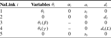
Notes: $\theta _1$
is the angle of the rotary device.
$\theta _1$
is the angle of the rotary device. $\theta _3$
,
$\theta _3$
, $\theta _4$
are the angles of the parallel working arms after equivalence, as in Eqs. (1) and (2)
$\theta _4$
are the angles of the parallel working arms after equivalence, as in Eqs. (1) and (2) $\beta$
,
$\beta$
, $\gamma$
.
$\gamma$
. $s_3$
is the offset of the static platform of the parallel working arm from the rotary device.
$s_3$
is the offset of the static platform of the parallel working arm from the rotary device. $s_5$
is the offset of the sprue from the center of the moving platform along the
$s_5$
is the offset of the sprue from the center of the moving platform along the $X_4$
-axis.
$X_4$
-axis. $d_2$
is the vertical distance between the center of the rotary device and the static platform.
$d_2$
is the vertical distance between the center of the rotary device and the static platform.
Substituting D-H parameter of Table II into Eq. (9), the transformation matrix of joints 1, 2, and 5 can be obtained:
 \begin{equation} \begin{gathered} \begin{aligned}{}_1^0T = \left [{\begin{array}{c@{\quad}c@{\quad}c@{\quad}c}{c{\theta _1}}&{ - s{\theta _1}}&0&{{s_1}}\\[5pt] {s{\theta _1}}&{c{\theta _1}}&0&0\\[5pt] 0&0&1&0\\[5pt] 0&0&0&1 \end{array}} \right ],{}_2^1T = \left [{\begin{array}{c@{\quad}c@{\quad}c@{\quad}c} 1&0&0&0\\[5pt] 0&1&0&0\\[5pt] 0&0&1&{{d_2}}\\[5pt] 0&0&0&1 \end{array}} \right ],{}_5^4T = \left [{\begin{array}{c@{\quad}c@{\quad}c@{\quad}c} 1&0&0&{{s_5}}\\[5pt] 0&1&0&0\\[5pt] 0&0&1&0\\[5pt] 0&0&0&1 \end{array}} \right ]\ \end{aligned} \end{gathered} \end{equation}
In the designing of parallel mechanism, we introduced the micro-displacement method [Reference Zhang, Xu, Yao and Zhao34] mentioned above to describe the transformation matrix ${}_4^2T$
between
${}_4^2T$
between $O_2$
to
$O_2$
to $O_4$
:
$O_4$
:
 \begin{equation} \begin{gathered} \begin{aligned}{}_4^2T = \left [{\begin{array}{c@{\quad}c}{{}^{\textrm{A}}{R_{\textrm{B}}}}&{{}^{\textrm{A}}{P_{\textrm{B}}}}\\[5pt] 0&1 \end{array}} \right ]\\[5pt] = \left [{\begin{array}{c@{\quad}c@{\quad}c@{\quad}c}{\cos \beta }&{\sin \beta \sin \gamma }&{\sin \beta \cos \gamma }&{{\textrm{L}}\tan \beta }\\[5pt] 0&{\cos \gamma }&{ - \sin \gamma }&0\\[5pt] { - \sin \beta }&{\cos \beta \sin \gamma }&{\cos \beta \cos \gamma }&{\textrm{L}}\\[5pt] 0&0&0&1 \end{array}} \right ] \end{aligned} \end{gathered} \end{equation}
From this, the pose matrix ${}_5^0T$
of the end pouring nozzle in the global coordinate system can be obtained according to Eqs. (10) and (11):
${}_5^0T$
of the end pouring nozzle in the global coordinate system can be obtained according to Eqs. (10) and (11):
 \begin{equation} \begin{gathered} \begin{aligned}{}_5^0T ={}_1^0T{}_2^1T{}_4^2T{}_5^4T = \left [{\begin{array}{c@{\quad}c@{\quad}c@{\quad}c}{{n_x}}&{{o_x}}&{{a_x}}&{{p_x}}\\[5pt] {{n_y}}&{{o_y}}&{{a_y}}&{{p_y}}\\[5pt] {{n_z}}&{{o_z}}&{{a_z}}&{{p_z}}\\[5pt] 0&0&0&1 \end{array}} \right ] \end{aligned} \end{gathered} \end{equation}
where each parameter is:
 \begin{equation*}\left \{ \begin {array}{l} {n_x} = \cos {\theta _1}\cos \beta \\[5pt] {n_y} = \sin {\theta _1}\cos \beta \\[5pt] {n_z} = - \sin \beta \\[5pt] {o_x} = \cos {\theta _1}\sin \beta \sin \gamma - \sin {\theta _1}\cos \gamma \\[5pt] {o_y} = \cos {\theta _1}\cos \gamma + \sin {\theta _1}\sin \beta \sin \gamma \\[5pt] {o_z} = \sin \beta \sin \gamma \end {array} \right .\begin {array}{*{20}{c}} {}&\begin {array}{l} {a_x} = \sin {\theta _1}\sin \gamma + \cos {\theta _1}\sin \beta \cos \gamma \\[5pt] {a_y} = \sin {\theta _1}\sin \beta \cos \gamma - \cos {\theta _1}\sin \gamma \\[5pt] {a_z} = \cos \beta \cos \gamma \\[5pt] {p_x} = {{\textrm {s}}_1} + {s_5}\cos {\theta _1}\cos \beta + L\cos {\theta _1}\tan \beta \\[5pt] {p_y} = {s_5}\sin {\theta _1}\cos \beta + L\sin {\theta _1}\tan \beta \\[5pt] {p_z} = {d_2} + L - {s_5}\sin \beta \end {array} \end {array}\end{equation*}
After simplifying and organizing Eq. (12), $p_x$
and
$p_x$
and $p_y$
, we obtain
$p_y$
, we obtain
 \begin{equation} \begin{gathered} \begin{aligned} \left \{{\begin{array}{*{20}{l}}{{p_x} -{{\textrm{s}}_1} = \left ({{s_5}\cos \beta + z\tan \beta } \right )\cos{\theta _1}}\\[5pt] {{p_y} = \left ({{s_5}\cos \beta + z\tan \beta } \right )\sin{\theta _1}} \end{array}} \right. \end{aligned} \end{gathered} \end{equation}
From this, we can obtain, ${\theta _1} = \pi \pm \arctan \left ({{p_y}/({p_x} -{s_1})} \right )$
.
${\theta _1} = \pi \pm \arctan \left ({{p_y}/({p_x} -{s_1})} \right )$
.
According to Eqs. (10)–(13), the inverse solution of the hybrid mechanism can be obtained as follows:
 \begin{equation} \begin{gathered} \begin{aligned} \left \{ \begin{array}{l}{\theta _1} = \pi \pm \arctan \left ({{p_y}/({p_x} -{s_1})} \right )\begin{array}{*{20}{c}}{}&{}&{} \end{array}\begin{array}{*{20}{c}}{}&{ - \pi \le{\theta _1} \le \pi } \end{array}\\[5pt] {d_2} ={{\textrm{p}}_z} - z -{s_5}\sin \beta \begin{array}{*{20}{c}}{\begin{array}{*{20}{c}}{\begin{array}{*{20}{c}}{}&{} \end{array}}&{} \end{array}}&{}&{}&{300 \le{d_2} \le 600} \end{array}\\[5pt] {\theta _3} = \beta = f(\beta )\begin{array}{*{20}{c}}{\begin{array}{*{20}{c}}{\begin{array}{*{20}{c}}{}&{} \end{array}}&{} \end{array}}&{}&{}&{} \end{array}\begin{array}{*{20}{c}}{}&{ - \pi/18 \le{\theta _3} \le \pi/18} \end{array}\\[5pt] {\theta _4} = \gamma = \arcsin ( \!-\!{{\textrm{p}}_y}/{{\textrm{e}}_v})\begin{array}{*{20}{c}}{}&{}&{\begin{array}{*{20}{c}}{}&{} \end{array}}&{0 \le \gamma \le \pi/2} \end{array}\\[5pt] {d_4} = z = \left ({\left ({{{\textrm{p}}_y}/\sin{\theta _1}} \right ) -{s_5}} \right )\tan \beta \begin{array}{*{20}{c}}{\begin{array}{*{20}{c}}{}&{} \end{array}}&{500 \le z \le 1000} \end{array} \end{array} \right. \end{aligned} \end{gathered} \end{equation}
3.2. Control system
Because the parallel robot control has the characteristics of nonlinearity, high coupling, and multiple inputs [Reference Craig39], and considering that at the high pouring temperature, it is difficult to achieve sensing detection. Semi-physical simulation control technology, also known as HIL, can simulate high temperatures, high pressures, reactions, and other general laboratory or training devices that cannot be carried out in the process, to achieve real-time interaction between the physical and simulation models, to produce a more realistic input and output response [Reference Yu, Han, Qu and Yang42, Reference Kelemena, Kelemenováa, Virgala, Miková and Lipták43]. Therefore, a vision-based semi-physical simulation pouring control system is proposed by us to solve the problem of poor flexibility of the pouring system and the difficulty of real-time control of the pouring process according to the pouring model.
The physical model of the ROS system is combined with virtual and real software control systems for real-time feedback tracking control, as shown in Fig. 8. The whole system includes the preprocessing layer, human-computer interaction layer, software control layer, and display layer. The function of the preprocessing layer is to obtain the standard model size by performing a three-dimensional geometric reconstruction of the prototype model and then import it into the ROS system to complete real-time attitude-tracking control on the display layer.

Figure 8. Block diagram of the hardware-in-the-loop simulation control system.
The software control layer is the core of the entire system. It mainly uses MATLAB/Simulink programming software to build the control system platform. According to actual requirements, the system is divided into a kinematics inverse solution module, servo three-loop PID control module, a communication module, and a vision module. Using the software’s excellent embedded packaging characteristics, the program structure is open and concise, convenient for secondary development [Reference Zhuqing44]. The software control system is shown in Fig. 9. Firstly, according to the position of the sandbox under the global coordinate system, the robot moves to the pouring station. After that, the vision module detects the position of the sandbox and kinematics inverse solution module the end point position of the ladle according to the dynamic model parameters of the ladle. Finally, the servo three-loop PID control module controls the joints of the hybrid working arm to reach the pouring position of the ladle and realizes the pouring task.

Figure 9. MATLAB/Simulink software control system of pouring robot.

Figure 10. MATLAB/Simulink software control system of pouring robot. The design block diagram of the three-loop PID controller of the servo system.

Figure 11. The analysis results of the equivalent workspace for the hybrid working arm.

Figure 12. In the figure, $qi, Vi, and ai$
represent the displacements, velocities, and accelerations of the four supporting branches, respectively. The true values of velocity and angular velocity are denoted as speed and acceleration. Furthermore, z, vz, and az represent the set values for the displacement, speed, and acceleration of the mold’s center in the pouring process. The four parameters at the top of the figure are the rotation angle
$qi, Vi, and ai$
represent the displacements, velocities, and accelerations of the four supporting branches, respectively. The true values of velocity and angular velocity are denoted as speed and acceleration. Furthermore, z, vz, and az represent the set values for the displacement, speed, and acceleration of the mold’s center in the pouring process. The four parameters at the top of the figure are the rotation angle $\theta _1$
of the hybrid working arm relative to the zero point, the increment of lifting height d2, the distance z between the parallel working arm’s dynamic and static platform, and the rotation angle
$\theta _1$
of the hybrid working arm relative to the zero point, the increment of lifting height d2, the distance z between the parallel working arm’s dynamic and static platform, and the rotation angle $\theta _3$
of the ladle.
$\theta _3$
of the ladle.

Figure 13. Fixed-point pouring test environment platform.
Although the traditional three-loop PID control system has good control performance, it is difficult to measure and calculate by the method of accurate mathematical model of the object, because the technical difficulty and workload are relatively large [Reference Hongqiang and Shuyou45, Reference Lee46]. To solve this problem, based on the aforementioned kinematics model, in this paper, we adopted the method that combined the cSPACE control board and MATLAB/Simulink to create an embedded rapid development environment. And we proposed a HIL simulation control based on a servo three-loop PID self-tuning controller, which shortens the development time of the robot. The frame of the device is shown in Fig. 10. $\theta ^*$
represents the reference angle input signal,
$\theta ^*$
represents the reference angle input signal, $w^*$
represents the reference angular velocity input signal,
$w^*$
represents the reference angular velocity input signal, $I ^*$
represents the reference current input signal,
$I ^*$
represents the reference current input signal, $\theta$
represents the motor angle output signal and
$\theta$
represents the motor angle output signal and $q$
represents the joint position output signal.
$q$
represents the joint position output signal.
3.3. Simulation analysis
3.3.1. Workspace analysis
The analysis of the workspace of a hybrid robotic system is crucial for evaluating its motion capabilities and applicability. Therefore, this subsection introduces the methods and results of the workspace analysis conducted on the hybrid robotic system.
First, we solve the spatial geometry using the known geometric equivalent model shown in Fig. 7 and Eq. (12). Next, based on the range of values from Table II and Eq. (14), a Monte Carlo method is employed for the accessibility analysis. The results, as shown in Fig. 11, illustrate the workspace of the robot as follows:
 \begin{equation*}\left \{ {\begin {array}{*{20}{c}} { - 420{\it mm} \le X \le 520{\it mm}}\\[5pt] { - 480{\it mm} \le Y \le 480{\it mm}}\\[5pt] {800{\it mm} \le Z \le 1600{\it mm}} \end {array}} \right .\end{equation*}
As shown in Fig. 11(b), the reachable space of the robot’s end effector nozzle is within the range of the sandbox, and it is capable of dispensing multiple workstations in a single stationary stop, meeting the operational requirements.
3.3.2. Performance parameter testing and analysis of each branch chain of 2UPR-2RPU
According to Eqs. (1)–(8), simplify the inverse solution as follows:
 \begin{equation} {q_i} = \sqrt{{\lambda _i}^2 +{\mu _i}^2} \end{equation}
where
 \begin{equation*}\left \{ {\begin {array}{*{20}{l}} {{\lambda _1} = z\sec \beta - {a_1}\sin \gamma \begin {array}{*{20}{c}} ;&{{\mu _1} = {a_2} - {a_1}\cos \gamma } \end {array}}\\[2pt] {{\lambda _2} = {a_4} - {a_3}\cos \beta + z\tan \beta \begin {array}{*{20}{c}} ;&{{\mu _3} = z + {a_3}\sin \beta } \end {array}}\\[2pt] {{\lambda _3} = z\sec \beta + {a_1}\sin \gamma \begin {array}{*{20}{c}} ;&{{\mu _2} = {a_1}\cos \gamma - {a_2}} \end {array}}\\[2pt] {{\lambda _4} = {a_3}\cos \beta + z\tan \beta - {a_4}\begin {array}{*{20}{c}} ;&{{\mu _4} = z - {a_3}\sin \beta } \end {array}} \end {array}} \right .\end{equation*}
Based on Eq. (15) and Table I, the zero state is obtained with $q_1$
= 60.4 cm,
$q_1$
= 60.4 cm, $q_2$
=
$q_2$
= $q_3$
= 44.4 cm, and
$q_3$
= 44.4 cm, and $q_4$
= 49.3 cm. These initial position data are inputted into the semi-physical simulation system shown in Fig. 9 for testing. The performance of each supporting branch is observed by setting the robot to extend the pouring mold forward in two stages. The velocities are set to 1 and 5 mm/s, respectively.
$q_4$
= 49.3 cm. These initial position data are inputted into the semi-physical simulation system shown in Fig. 9 for testing. The performance of each supporting branch is observed by setting the robot to extend the pouring mold forward in two stages. The velocities are set to 1 and 5 mm/s, respectively.
The results, as depicted in Fig. 12, demonstrate that the robot in the semi-physical simulation system can accurately achieve the desired pose. Under the displacement of stages $\bigcirc\!\!\!\!1\,$
and
$\bigcirc\!\!\!\!1\,$
and $\bigcirc\!\!\!\!2\,$
, the displacements, velocities, and accelerations of each supporting branch remain within a reasonable range during the intermediate motion. However, during the initial and final movements, there may be a significant increase in end effector load, resulting in larger variations in speed and angular velocity.
$\bigcirc\!\!\!\!2\,$
, the displacements, velocities, and accelerations of each supporting branch remain within a reasonable range during the intermediate motion. However, during the initial and final movements, there may be a significant increase in end effector load, resulting in larger variations in speed and angular velocity.
4. Experiment studies
4.1. Initial test
In order to verify the feasibility and effectiveness of the HIL simulation control system design for the pouring robot, a prototype test environment platform is constructed, as shown in Fig. 13.
Table III. Key parameter preliminary selection test data.


Figure 14. Initial test part of test paper wetting test results.
Because the iron pouring process is complex, costly, and difficult to control the safety. Therefore, we verify the feasibility of the vision-based HIL control system through water simulation [Reference Lee46]–[Reference Viswanath, Manu, Savithri and Pillai47] pouring tests. Considering that the filling capacity and fluidity of the pouring liquid [Reference Ingle and Narkhede48] affect the quality of pourings during the pouring process, the key parameter test variables are designed through the control variable method according to the test requirements that the pouring robot control system can meet.
The purpose is to find the appropriate drop point (pouring nozzle position), and the amount of external drop of the pouring liquid under different test variables $Z_{DE}$
,
$Z_{DE}$
, $Y_{DE}$
,
$Y_{DE}$
, $\beta$
,
$\beta$
, $V_S$
.
$V_S$
. $Z_{DE}$
, and
$Z_{DE}$
, and $Y_{DE}$
, respectively, represents the vertical and horizontal distances between the pouring nozzle and the liquid collection bucket A, when the ladle rotation angle
$Y_{DE}$
, respectively, represents the vertical and horizontal distances between the pouring nozzle and the liquid collection bucket A, when the ladle rotation angle $\beta$
=40
$\beta$
=40 $^{\circ }$
;
$^{\circ }$
; $v_q$
represents the rotation speed of the ladle when it is dumped;
$v_q$
represents the rotation speed of the ladle when it is dumped; $v_{bs}$
represents the rotation speed of the ladle when it is dumped;
$v_{bs}$
represents the rotation speed of the ladle when it is dumped; $V_S$
pouring the remaining pouring liquid volume in the bag.
$V_S$
pouring the remaining pouring liquid volume in the bag.
-
• Initial test: The actual test pouring liquid will be spilled to the outside before being poured into the pouring nozzle position, which is defined as the amount of external dripping. The method of preliminary judgment of the external drop volume $Q_d$
is through 17 tests on the area of the test paper infiltrated by the red ink (representing the pouring liquid), as shown in TableIII. In the process, we ensured that the value of
$Q_d$
is as small as possible. The test results are shown in Fig. 14. Four sets of tests are carried out. After eliminating the wrong test, it is ensured that the pouring liquid trace falls near the center of the liquid collection bucket A. Comparing tests T1, T4, T5, T7, while
$\beta$
,
$V_s$
, and Ladle are static,
$Y_{DE}$
or
$Z_{DE}$
becomes larger, the wetted area of the test paper will increase, and
$Q_d$
will increase. However, comparing tests T15, T11, T8, when the range of the dumping angle becomes smaller, the value of
$Q_d$
also decreases.
$Q_d$
is through 17 tests on the area of the test paper infiltrated by the red ink (representing the pouring liquid), as shown in TableIII. In the process, we ensured that the value of
$Q_d$
is as small as possible. The test results are shown in Fig. 14. Four sets of tests are carried out. After eliminating the wrong test, it is ensured that the pouring liquid trace falls near the center of the liquid collection bucket A. Comparing tests T1, T4, T5, T7, while
$\beta$
,
$V_s$
, and Ladle are static,
$Y_{DE}$
or
$Z_{DE}$
becomes larger, the wetted area of the test paper will increase, and
$Q_d$
will increase. However, comparing tests T15, T11, T8, when the range of the dumping angle becomes smaller, the value of
$Q_d$
also decreases. -
• Parameter test: According to the above external dripping test, to ensure the appropriate test parameter range, set the rotation angle of each group of test ladle 40 60
$^{\circ }$
. At the same time, in order to avoid the influence of the surface tension of the remaining pouring liquid in the ladle on the experimental results. After the end of the test, drip for three minutes to ensure the synchronization of the test data. The measuring unit adopts two electronic scales with different precisions. The test uses the liquid collection bucket A to replace the sprue cup and sandbox. The liquid collected by the liquid collection bucket A indicates the actual quality of the pouring liquid required for the blank, and the liquid collected by the liquid collection bucket B indicates the initial dumping. The amount of external drops at the end. At the end of each test, the quality change is obtained through the electronic scale. The test parameter settings and results are shown in Table IV.


4.2. Comparative experiment of dynamic water simulation pouring
4.2.1. Pouring liquid height
$Z_{DE}$

During the test, when the pouring parameters $Z_{DE}$
and
$Z_{DE}$
and $Y_{DE}$
are set improperly, it will cause a large amount of pouring liquid to splash out of the liquid collection bucket A. Therefore, according to the initial test, the appropriate
$Y_{DE}$
are set improperly, it will cause a large amount of pouring liquid to splash out of the liquid collection bucket A. Therefore, according to the initial test, the appropriate $Z_{DE}$
is set to select the appropriate range of 40–60 cm. And then the mass changes of
$Z_{DE}$
is set to select the appropriate range of 40–60 cm. And then the mass changes of $P_A$
and
$P_A$
and $P_B$
before and after the liquid collection buckets A and B account for the percentage of the total outflow of the pouring liquid
$P_B$
before and after the liquid collection buckets A and B account for the percentage of the total outflow of the pouring liquid $P_{AB}$
. The histogram of the change with
$P_{AB}$
. The histogram of the change with $Z_{DE}$
and different pouring liquid heights correspond to the intermediate state of pouring, as shown in Figs. 15(a) and 16(a).
$Z_{DE}$
and different pouring liquid heights correspond to the intermediate state of pouring, as shown in Figs. 15(a) and 16(a).
Table IV. Performance parameter test of water simulation pouring robot.
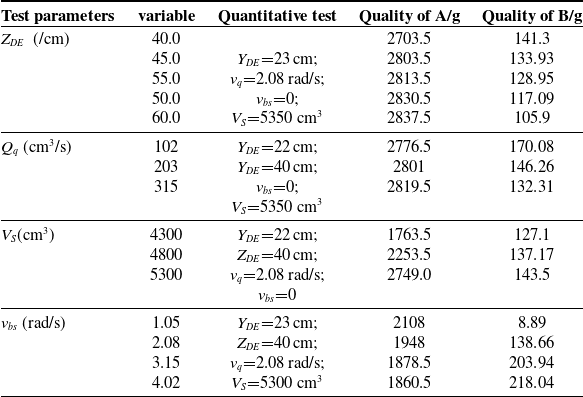

Figure 15. The ratio of $P_A$
and
$P_A$
and $P_B$
to
$P_B$
to $P_{AB}$
(a). Pouring liquid height
$P_{AB}$
(a). Pouring liquid height $Z_{DE}$
changes. (b). The average flow rate of the pouring liquid
$Z_{DE}$
changes. (b). The average flow rate of the pouring liquid $Q_q$
changes. (c). Volume change in the ladle before pouring
$Q_q$
changes. (c). Volume change in the ladle before pouring $V_S$
. (d). The
$V_S$
. (d). The $v_{bs}$
changes after the pouring simulation is completed.
$v_{bs}$
changes after the pouring simulation is completed.

Figure 16. (a). Diagram of the intermediate state under pouring at different heights. (b). Three state diagrams of pouring under different flow rates. (c). Pouring state at the same time and pose when different $V_s$
.
$V_s$
.
The results show that, when the pouring liquid height is in the range of 40–45 cm, the distance between the pouring nozzle and the liquid collection bucket is relatively close. At this time, the trajectory of the pouring liquid just leaving the pouring nozzle is a curve, so as the $Z_{DE}$
increases the mass of the liquid collection bucket A and the liquid collection bucket B The change is nonlinear; when the pouring liquid height is in the range of 45–60 cm, the distance between the pouring nozzle and the liquid collection bucket is relatively long, and the pouring liquid trajectory is almost straight at this time, so the mass change of the liquid collection bucket A and the liquid collection bucket B is linear with the change of
$Z_{DE}$
increases the mass of the liquid collection bucket A and the liquid collection bucket B The change is nonlinear; when the pouring liquid height is in the range of 45–60 cm, the distance between the pouring nozzle and the liquid collection bucket is relatively long, and the pouring liquid trajectory is almost straight at this time, so the mass change of the liquid collection bucket A and the liquid collection bucket B is linear with the change of $Z_{DE}$
Negative correlation.
$Z_{DE}$
Negative correlation.
4.2.2. The average flow rate of pouring ladle
$Q_q$

Select the appropriate pouring height $Z_{DE}$
=40 cm through the above experimental results. The control variable of this summary is the flow rate of pouring ladle, and the position relationship of the upper and lower branches of the parallel working arm is adjusted through the speed loop of the control system. When considering the appropriate speed so that the pouring liquid can be completely poured into the liquid collection bucket A, set the average flow rate of pouring liquid
$Z_{DE}$
=40 cm through the above experimental results. The control variable of this summary is the flow rate of pouring ladle, and the position relationship of the upper and lower branches of the parallel working arm is adjusted through the speed loop of the control system. When considering the appropriate speed so that the pouring liquid can be completely poured into the liquid collection bucket A, set the average flow rate of pouring liquid $Q_1$
=112 cm3/s,
$Q_1$
=112 cm3/s, $Q_2$
=223 cm3/s,
$Q_2$
=223 cm3/s, $Q_3$
=345 cm3/s. In the experiment, the changes in the quality of the collected liquid and its three states before, during, and after pouring are obtained, as shown in Figs. 15(b) and 16(b).
$Q_3$
=345 cm3/s. In the experiment, the changes in the quality of the collected liquid and its three states before, during, and after pouring are obtained, as shown in Figs. 15(b) and 16(b).
The results show that, when the ladle flow changes uniformly, there is a linear negative correlation between the mass changes of the liquid collection buckets A and B. The three states show that the $Q_1$
pouring liquid trajectory is the most stable, but the pouring time is long, and the external overflow is large; the
$Q_1$
pouring liquid trajectory is the most stable, but the pouring time is long, and the external overflow is large; the $Q_3$
pouring speed is fast, but the pouring liquid trajectory is thick and unstable; the
$Q_3$
pouring speed is fast, but the pouring liquid trajectory is thick and unstable; the $Q_2$
pouring speed is moderate and the pouring liquid trajectory has a relatively large pouring process. Good smoothness and stability.
$Q_2$
pouring speed is moderate and the pouring liquid trajectory has a relatively large pouring process. Good smoothness and stability.
4.2.3. Pouring liquid volume
$V_s$

Through the above two sets of experiments, $Z_{DE}$
=40 cm and
$Z_{DE}$
=40 cm and $Q_q$
=223 cm3/s are selected to ensure a smooth and stable pouring liquid trajectory. By changing the volume of the ladle
$Q_q$
=223 cm3/s are selected to ensure a smooth and stable pouring liquid trajectory. By changing the volume of the ladle $V_s$
, the mass change of the two liquid collection buckets is obtained, as shown in Fig. 15(c). Given the difference in flow rate during pouring of different volumes, the pouring states at the same time and pose are selected, as shown in Fig. 16(c).
$V_s$
, the mass change of the two liquid collection buckets is obtained, as shown in Fig. 15(c). Given the difference in flow rate during pouring of different volumes, the pouring states at the same time and pose are selected, as shown in Fig. 16(c).
The results show that, with the change of $V_s$
, there is a nonlinear positive correlation between the mass change of the liquid collection buckets A and B. And under the same posture, the larger the volume
$V_s$
, there is a nonlinear positive correlation between the mass change of the liquid collection buckets A and B. And under the same posture, the larger the volume $V_s$
in the ladle, the larger the corresponding flow in the early period, the smaller the flow in the middle period, and the same in the later period.
$V_s$
in the ladle, the larger the corresponding flow in the early period, the smaller the flow in the middle period, and the same in the later period.
4.2.4. Ladle tilting speed
$v_{bs}$

Select $Z_{DE}$
=40 cm,
$Z_{DE}$
=40 cm, $Q_q$
=223 cm3/s, and
$Q_q$
=223 cm3/s, and $V_s$
=5300 cm3 according to the above three sets of test results to ensure that the pouring liquid track is smooth and stable and the pouring liquid is continuous in a single test. By setting the ladle tilting speed
$V_s$
=5300 cm3 according to the above three sets of test results to ensure that the pouring liquid track is smooth and stable and the pouring liquid is continuous in a single test. By setting the ladle tilting speed $v_{bs1}$
=0.0182 rad/s,
$v_{bs1}$
=0.0182 rad/s, $v_{bs2}$
=0.0363 rad/s,
$v_{bs2}$
=0.0363 rad/s, $v_{bs3}$
=0.0569 rad/s,
$v_{bs3}$
=0.0569 rad/s, $v_{bs4}$
=0.0793 rad/s for experimental research, the mass change of the two liquid collocation buckets is obtained, as shown in Fig. 15(d).
$v_{bs4}$
=0.0793 rad/s for experimental research, the mass change of the two liquid collocation buckets is obtained, as shown in Fig. 15(d).
The results show that, with the uniform increase of $v_{bs}$
, there is a linear negative correlation between the mass changes of the liquid collection buckets A and B, and when the
$v_{bs}$
, there is a linear negative correlation between the mass changes of the liquid collection buckets A and B, and when the $v_{bs}$
is small, the pouring liquid does not drip to the liquid collection B at the end of pouring.
$v_{bs}$
is small, the pouring liquid does not drip to the liquid collection B at the end of pouring.
5. Conclusions
Based on the research of pouring mechanism, this paper designs and develops a movable hybrid pouring robot with compact structure, which solves the problem of fixed positions of pouring devices at home and abroad and can meet the intelligent pouring tasks of small and medium-sized castings.
The kinematics model of the parallel working arm is established using the micro-displacement method. Based on this, the equivalent method and the D-H method are used to determine the pose of the end ladle, which reduces the control complexity and calculation amount and simplifies the modeling process. The HIL control strategy of the pouring robot is designed, and the software and hardware control system platform is built. Subsequently, the robot’s workspace, −42 cm $\leq$
X
$\leq$
X $\leq$
52 cm, −48 cm
$\leq$
52 cm, −48 cm $\leq$
X
$\leq$
X $\leq$
48 cm, −80 cm
$\leq$
48 cm, −80 cm $\leq$
X
$\leq$
X $\leq$
160 cm, satisfying the on-site application requirements, was obtained using the Monte Carlo method. Comparative experiments of the key performance parameters of the parallel working arm’s four supporting branches were conducted using the established semi-physical simulation system, thereby validating the rationality of the structural design and kinematic analysis.
$\leq$
160 cm, satisfying the on-site application requirements, was obtained using the Monte Carlo method. Comparative experiments of the key performance parameters of the parallel working arm’s four supporting branches were conducted using the established semi-physical simulation system, thereby validating the rationality of the structural design and kinematic analysis.
Through the performance test of the control system, four sets of water simulation fixed-point pouring tests were designed. And four pouring dynamic parameter ranges were determined during fixed-point pouring, the pouring liquid height, the average flow rate of pouring liquid, the pouring liquid volume, and the ladle tilting speed: $Z_{DE}$
=35–40 cm,
$Z_{DE}$
=35–40 cm, $Q_q$
=112 cm3/s,
$Q_q$
=112 cm3/s, $V_s$
=5300 cm3,
$V_s$
=5300 cm3, $v_{bs}$
=0.0182 rad/s. The research results show that the pouring under the above conditions can ensure smooth and stable pouring liquid trajectory, less external dripping, moderate pouring flow, and can complete multiple pouring tasks with different qualities of castings.
$v_{bs}$
=0.0182 rad/s. The research results show that the pouring under the above conditions can ensure smooth and stable pouring liquid trajectory, less external dripping, moderate pouring flow, and can complete multiple pouring tasks with different qualities of castings.
Supplementary material
The supplementary material for this article can be found at http://dx.doi.org/10.1017/S0263574723001881.
Author contributions
Chengjun Wang and Hao Duan conceived and designed the study. Hao Duan modeled, analyzed, and built a control system for the robot. Chengjun Wang and Hao Duan jointly wrote this article, and Long Li and Hao Duan jointly completed the experimental part of this article. In addition, Long Li also provides guidance on paper writing.
Financial support
This work was supported in part by the National Innovation Method Work Special Project (NO.2018IM010500), Collaborative Innovation Project of Universities in Anhui Province (NO.GXXT2019018), and Science and Technology Major Special Program Project in Anhui Province (NO.16030901012).
Competing interests
The authors declare none.
Ethical approval
Not applicable.


