


Political scientists are no strangers to duration models, which allow researchers to test hypotheses about how long until an event of interest occurs. Box-Steffensmeier and Jones’ (Reference Box-Steffensmeier and Jones2004) work on duration models arguably marks the watershed moment for these models’ use in political science. The main virtue of the models is the ease with which they handle potential duration dependence—formally, that the likelihood of an event may be contingent on how long a subject has been at risk.Footnote 1
We both work frequently with duration models; accordingly, we happily field duration model–related queries from our colleagues and students. In doing so, we were struck by how often we receive the same questions, which cluster into the following three groups:
1. People asking how duration models “work” and then being surprised when we use other models to explain (e.g., logit or probit).
2. People asking how to interpret duration models. Usually, this manifests as (1) a preoccupation with one specific interpretation strategy, without seeing how different interpretation methods are related; or (2) being overwhelmed with the number of possible interpretation strategies and lacking a clear sense of where to begin.
3. People asking how to compute a duration model quantity in R or Stata.
With these frequent queries in mind, we searched for a piece or two that succinctly organized and summarized our answers in one place. To our surprise, no such piece existed.
This article synthesizes our more frequent answers. Our answers’ overarching theme is that duration models are a type of regression model and, as such, most of the general intuition and best practices gleaned from linear regression models, logit models, and others apply equally. Duration models have an extra “wrinkle” or two because they can address right-censored data; however, these wrinkles are accommodated automatically when using the models. There is nothing otherwise unique or special about duration models’ underlying principles that should lead practitioners to jettison their intuition when estimating them.Footnote 2 Appreciating this point is important because many of the best practices and rules of thumb internalized by practitioners in the context of other regression models are inconsistently heeded in the context of duration models. As a notable example, reporting p-values or confidence intervals around predicted probabilities from a logit or probit model is ubiquitous, whereas reporting similar measures of uncertainty from a duration model is inconsistent at best, as we illustrate with two meta-analyses.
Not recognizing the connection between duration and other regression models also has negatively affected whether and how scholars interpret their duration model results. For instance, some researchers simply stop after interpreting the model’s estimated coefficients. When substantive interpretation does happen, practitioners use various strategies with varying degrees of success. The plethora of interpretation strategies seems to deepen the uncertainty and mystery surrounding the models.
To engage with these issues, we present four stylized maxims about interpreting duration models that represent major areas where practitioners’ use of them might go awry. We articulate these maxims by drawing parallels to more widely used regression models to emphasize our central point: the hard-won intuition that practitioners have developed with other regression models applies equally to duration models. Our maxims advise practitioners to move beyond the regression table when interpreting duration models. We categorize existing duration model interpretation strategies to provide practitioners with a concise overview—an important organizational exercise that does not exist elsewhere.Footnote 3 Following this overview, we encourage practitioners to use their paper’s substance and theory when deciding which interpretation strategy to employ while also underscoring the universal importance of measures of uncertainty. We conclude by assessing the various interpretation strategies’ strengths and weaknesses in terms of presenting and interpreting the results, followed by providing more general guidance for how to use these interpretation strategies in conjunction with one another to maximize their effect.
Our maxims advise practitioners to move beyond the regression table when interpreting duration models. We categorize existing duration model interpretation strategies to provide practitioners with a concise overview—an important organizational exercise that does not exist elsewhere.
THE MAXIMS
#1: You Cannot Directly Interpret the Coefficients as Substantive Effects
Regardless of which duration model you estimate,Footnote 4 all duration models with covariates are nonlinear in parameters—the same as logits, probits, and count models, among others. Therefore, we cannot directly interpret the magnitude of any βs as we might in a simple additive linear regression model because they are not equivalent to the coefficients’ substantive effects (marginal or otherwise) on y. Instead, we must generate additional quantities to present our model’s substantive results (King, Tomz, and Wittenberg Reference King, Tomz and Wittenberg2000).
Stated simply, you cannot stop at the regression table. Our hypotheses are usually about x’s effect on y. However, in all nonlinear models, β does not tell us about the relationship between x and y but rather between x and y*.Footnote 5 To reach a conclusion about y, we need to convert y* back to the quantity we care about, y, through a link function. In a logit, applying the logistic link transforms y* into a new quantity, y (technically, Pr(y=1)), whose values fall between 0 and 1, yielding probabilities.Footnote 6 For duration models, the usual link function is exp(y*), which produces a y (≡ t) that must be greater than 0, as time cannot be negative. Without this link function, β represents x’s effect on either the log-hazard (for proportional hazard models) or the log-duration (for accelerated failure time models),Footnote 7 neither of which is likely to be the focus of our hypotheses. Therefore, you must transform the βs in some way to glean substantive meaning, as discussed in Maxim #2. How you should transform the βs is directly related to your hypothesis about x’s effect on y—specifically, the way in which you framed your discussion of y, as we discuss further in Maxim #3.
#2: To Generate Substantive Effects, You Will Need to Do “Something” to the Coefficients
There are several ways to substantively interpret duration-model results. Each interpretation is technically correct (see Maxim #3), which is both a blessing and a curse—no matter which strategy you choose, your inferences will be technically sound, but clear-cut standards cannot exist regarding when some strategies perform better than others. Therefore, determining the best strategy for your work entails getting a sense of what the different strategies are, how they relate to one another, and which questions a respective strategy allows you to address most easily.
We loosely group extant interpretation strategies along two dimensions. The first relates to the underlying quantity of interest. The second dimension pertains to whether the quantity is an absolute or a relative quantity. The result is four groupings, shown in table 1.
Table 1 Current Approaches to Substantive Interpretation
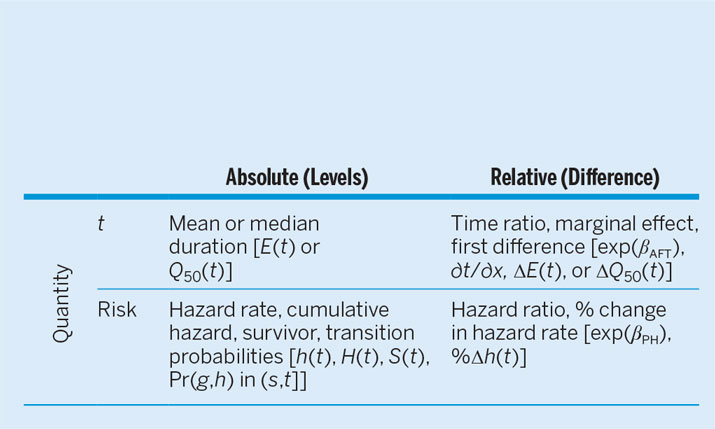
There are four noteworthy observations from the table:
1. All interpretation strategies involve either exponentiating the model’s βs or generating a predicted quantity using the βs, for reasons discussed in Maxim #1.
2. Duration models have two families of predicted quantities. These focus on how long until something occurs (i.e., the duration, t) or, equivalently, on the risk that something occurs (i.e., the hazard, h(t)); t and h(t) are the duration model equivalent of OLS’s predicted y $\left( {\hat{y}} \right)$.Footnote 8 For exposition purposes, think of hazards as being conceptually similar to probabilities, but also note the two are not usually synonyms.
3. Parametric duration models are built from asymmetric distributions, which means the mean and median survival times will not be equal. Observed survival times tend to be right-skewed, and the implications of computing any skewed variable’s mean versus median apply equally in a duration context. Furthermore, there may be right-censored subjects—subjects that will eventually experience the event of interest but have not experienced it yet when last observed.Footnote 9 Typically, right-censored observations fall in the right tail of t’s observed distribution.Footnote 10 As a general rule of thumb, the more right-censored subjects there are, the more appealing the median becomes.
4. There are numerous ways to quantify “risk” from a duration model, including the risk of an event occurring (the hazard, h(t)); the probability of an event not occurring (the survivor function, S(t)); the total risk that an event will have occurred (the cumulative hazard function, H(t)); and the probability that an event will have occurred (transition probabilities). Each of these is a different way to express the same underlying concern: how (un-)likely is it that an event will occur by some point in time.

Some of these quantities are easier to compute than others, depending on users’ statistical program of choice. We inventory R and Stata’s respective capabilities in appendix D.
#3: All of the Techniques Are Correct from a Technical Perspective, but Some Make More Sense Than Others
All of these interpretation strategies come from the same underlying model estimates (i.e., the βs and standard errors). Thus, all of these strategies are correct, from a technical perspective,Footnote 11 the same way that odds ratios and predicted probabilities are equally correct ways of interpreting logit output. Therefore, you must use other nontechnical criteria to guide decisions about which strategy to employ. We suggest considering two criteria, both relating to your paper’s presentation.
First, consider the extent to which a given interpretation strategy matches your theory and hypotheses. Reference Kropko and HardenKropko and Harden (forthcoming) make this point succinctly: If your hypothesis is framed in terms of durations—for instance, how long until a civil war recurs—then presenting your results in terms of durations logically follows (e.g., mean or median duration). Conversely, if your hypothesis is framed in terms of events (e.g., which factors make a civil war more likely to recur), then presenting the results in terms of risk-based quantities would be a better match. These quantities speak more directly to an event’s occurrence (or lack thereof) by depicting the conditions under which subjects are more likely to “survive”—here, that states remain at peace. Although our first point appears fairly simple and logical, misalignment between framing and interpretation strategies is rampant in political science. Reference Kropko and HardenKropko and Harden’s (forthcoming) meta-analysis of 80 articles using Cox duration models reveals that approximately 33 (41.25%) have predominantly duration frames and another 10 to 14 use both frames equally (12.5%–17.5%). However, none of these articles generate duration-based quantities for interpretation.
Second, consider the relative ease with which a particular post-estimation quantity allows you to present and interpret your results. Some techniques may be more straightforward for your audience to understand than others. We return to this point in our broader discussion of the various quantities’ strengths and weaknesses.
#4: Whatever Technique You Choose, You Will Need p-Values or Confidence Intervals
With duration models, as with other regression models, measures of uncertainty around our predicted quantities improve our ability to make inferences. Standard practice for logit/probit models is to report such measures around both the estimated coefficients and any predicted quantities. However, standard practice for duration models is much less consistent. A review of all articles in the Journal of Politics in 2017 underscores this point. Of these articles, 10 report at least one logit or probit model in the main text, and 9 of those 10 analyses generate a post-estimation quantityFootnote 12 with some measure of uncertainty, suggesting that this practice is well internalized.Footnote 13 In comparison, four articles estimate duration models, with measures of uncertainty reported less consistently. They are reported for any first differences and hazard ratios but not for survival curves.
This pattern holds more broadly: practitioners inconsistently report measures of uncertainty for duration model post-estimation quantities.
This pattern holds more broadly: practitioners inconsistently report measures of uncertainty for duration model post-estimation quantities. We examine all articles in the Journal of Politics, American Journal of Political Science, and American Political Science Review from 2012 to 2016 and assess whether they report (1) a Cox model in the main text, and (2) any post-estimation quantities in the main text.Footnote 14 There are 16 such articles,Footnote 15 of which four do not report any post-estimation quantities (25%).
Of the remaining 12 articles that do report post-estimation quantities,Footnote 16 hazard ratios appear most frequently (9 of 12), each time with a measure of uncertainty. However, hazard ratios have weaknesses stemming from being a measure of relative change, as we elaborate on in the next section. Five of these 12 articles report only hazard ratios (Cox’s “Rel” segment in figure 1), equivalent to a logit analysis reporting and interpreting odds ratios only. Finally, 6 of the 12 articles report a survivor curve (S(t)) and/or hazard rates (h(t)), but only one includes a measure of uncertainty around the quantity.Footnote 17

Figure 1 Meta-Analyses Comparison
Note: “CIs” used as shorthand for “any measure of uncertainty.”
Figure 1 visually depicts the two patterns from our two meta-analyses. The bars for both models should be filled entirely with the darkest gray if all articles report post-estimation quantities with measures of uncertainty. This is clearly not the case for duration models, indicating that the interpretation of duration models differs from similar models. This trend is troubling because without measures of uncertainty, drawing meaningful inferences from post-estimation quantities can be difficult.Footnote 18
GENERAL STRENGTHS AND WEAKNESSES
Although all of the quantities in table 1 are correct, they are not equally useful in all cases. Each has strengths and weaknesses in terms of ease of interpretation, for both the researcher and the audience. We discuss individual strengths and weaknesses in appendix B, but summarize several broader rules of thumb here. As we noted earlier, most of the following rules of thumb apply to post-estimation quantities from any regression model, not only duration models, but researchers often overlook this similarity.
• If you generate absolute quantities, you will have to generate at least two covariate profilesFootnote 19 with different x values. Otherwise, you will be unable to demonstrate how changes in x’s value bring about change in the predicted quantity—a necessity for substantive significance.
• Rainey (Reference Rainey2017) points out that predicted quantities do not automatically inherit the βs’ unbiased properties for any nonlinear regression model. Practitioners should be particularly mindful of biased predicted quantities when sample sizes are small.
• If you are looking at absolute quantities, the hazard and cumulative hazard are not scaled in especially intuitive units.Footnote 20 Comparatively speaking, duration-based quantities, the survivor, and transition probabilities have a far more intuitive scale, with the first scaled in the same units as the duration variable (e.g., months or years) and the survivor and transition probabilities expressed as probabilities.
• Relative measures expressed in terms of ratios or percentages can be misleading. For instance, say that increasing x’s value produces a 100% increase in the hazard rate. However, a 100% increase could result if h(t) increased in value from 0.4 to 0.8 (a fairly frequent event), but it also could result if the hazard increased from 0.00001 to 0.00002 (a very infrequent event). As Hanmer and Kalkan (Reference Hanmer and Ozan Kalkan2013, 265) point out, knowing something about the absolute level of the hazard, probability, or duration is “a necessary element for determining substantive significance.” Yet, figure 1 illustrates that linking absolute and relative quantities in duration models is rare. More Cox model articles report only a relative measure compared to those that report both relative and absolute measures (total “Rel” segment size > total “Rel + Abs” segment size).
Our advice is the same as Hanmer and Kalkan’s (Reference Hanmer and Ozan Kalkan2013) for reported quantities. We prefer using both absolute and relative quantities in general, and duration models are no exception. We typically begin by mentioning whether the coefficient is statistically different from zero. We then move to absolute quantities to give readers information about the quantity’s magnitude, calculating these absolute quantities for various covariate profiles of interest. We also usually check to see whether the profiles’ confidence intervals overlap with one another—although with caution because overlapping confidence intervals do not necessarily mean a lack of statistical significance (Austin and Hux Reference Austin and Hux2002; Bolsen and Thornton Reference Bolsen and Thornton2014; Schenker and Gentleman Reference Schenker and Gentleman2001).Footnote 21 Following this, we mention relative quantities to clearly and concretely communicate to readers the relative change in the quantity’s value. By the end, readers have the information they require to make judgments about our results’ substantive and statistical significance with relative ease.
CONCLUSION
Duration models’ usage has grown in political science, but researchers’ adeptness with them has grown at a slower rate. Many applications have been limited by a lack of clear best practices for substantively interpreting the models’ results. This article bridges these gaps by providing some rules of thumb to guide substantive interpretations of duration models. At its core, this set of maxims is built from a straightforward yet often underappreciated claim: duration models are like any other type of regression model with which political scientists work. As a result, almost all of the same guidance that political scientists receive with respect to interpreting a logit model, for instance, applies equally to duration models. Yet, our meta-analyses of published articles illustrate that this guidance is not applied to duration models as frequently as other models. Overall, then, the message is clear: political scientists can do better when it comes to interpreting duration models.
SUPPLEMENTARY MATERIAL
To view supplementary material for this article, please visit https://doi.org/10.1017/S104909651900060X
ACKNOWLEDGMENTS
The authors’ names appear in alphabetical order. Parts of this article were presented in the 2016–2017 International Methods Colloquium series and the University of Mississippi’s International Relations Workshop. We thank Daniel Kent for feedback. We bear sole responsibility for any remaining errors and shortcomings. All analyses were performed using Stata 14.2 unless otherwise noted.


