


Introduction
Nowadays, China is one of the 22 countries with a high burden of tuberculosis. Tuberculosis is the first common cause of death from infectious diseases [1]. In China, its incidence is second only to viral hepatitis in legal infectious diseases. Despite the great progress that has been made in controlling tuberculosis over the past decades, China is still among the countries with the highest burden of tuberculosis [Reference Xu2]. Although the case-finding rate is higher than 85% [Reference Li3] and the success rate of new smear-positive tuberculosis patients is higher than 90%, tuberculosis remains a major public health problem. The proportion of multi-drug resistant tuberculosis is still high, with 3.3% of new cases and 20% of retreatment cases have multi-drug resistant tuberculosis in the world [1]. The disease brings tremendous physical and psychological pain to the patient, which seriously affects their quality of life. It affects the therapeutic effect of the disease and physical recovery in turn [Reference Ding4]. Researches on infectious diseases such as tuberculosis are mostly limited to a single description of the incidence of diseases, neglecting the geographical relevance of the occurrence of tuberculosis and cannot make a certain discussion on the spatial distribution of disease from a quantitative level in China. While, tuberculosis as an infectious disease has certain links with the local environment, population, climate and so on. Its occurrence, development and epidemic are spatial phenomena with interactions and proliferation. In view of this, this study aims to investigate the clustering of pulmonary tuberculosis and study the influencing factors of the incidence of it, which in order to provide a theoretical basis for the formulation of public health policies in various regions, prevent and control tuberculosis and provide a reference for similar research.
Spatial information is used to extend the analysis of epidemic disease in spatial epidemiology [Reference Li, Xi and Ren5, Reference Pfeiffer6]. In order to predict the spatial-temporal trends of disease and the correlation between a disease and its latent factors, spatial epidemiology also explores the spatial distribution model [Reference Li, Xi and Ren5, Reference Jafari-Koshki, Arsang-Jang and Raei7, Reference Li and Wang8]. Quantitative methods can present the distribution characteristics of disease objectively and scan statistics can describe the clustering characteristics in terms of both space and time [Reference Kulldorff and Nagarwalla9–Reference Li and Wang11].
A meta-analysis of Bauer et al. [Reference Bauer, Leavens and Schwartzman12] found that, on a global scale, the overall quality of life of pulmonary tuberculosis patients is low. Not only the physical function is diminished, but also psychological, mental and social functions are greatly affected. In terms of social factors, Masumoto et al. [Reference Masumoto13] found that in addition to clinical factors, low socioeconomic status, including exposure to secondhand smoke and little social support, may be related to the quality of life of pulmonary tuberculosis patients through a cross-sectional survey. In terms of personal factors, by conducting semi-structured interviews, Rondags et al. [Reference Rondags14] found there are three main reasons for patients not complying with the treatment of pulmonary tuberculosis. The three main reasons include knowledge about tuberculosis, knowledge about tuberculosis treatment and choosing a healthcare treatment facility. In terms of environmental factors, Grange and Gandy [Reference Grange and Gandy15] considered that analysis of the prevalence of tuberculosis must take into account the effects of changes in the environment and ecological factors and it was necessary to determine whether pathogenic microorganisms were evolving.
This paper is organised as follows. In the section Materials and methods, from both spatial and temporal perspectives, we will analyse the status and trends of the incidence of pulmonary tuberculosis (IPT) in China during 2008–2015. Then, apply local spatial autocorrelation analysis to explore the spatial relationship of the IPT. In the section Results, we establish Spatial Lag Model. The last section contains the conclusions, the highlights and limitations of our model.
Materials and methods
Data source
We have 14 categories of data from 31 provinces in China in 2014. The 14 categories of data are (1) the IPT (1/100 000), (2) the proportion of people who go to high school (HS)(1/10 000), (3) household consumption levels (HCL)(yuan), (4) population mortality (PM)(1/1000), (5) the number of health technicians per 10 000 people (HT)(person), (6) the number of beds in medical institutions per 10 000 people (BMI)(person), (7) per capital gross regional product (PGDP)(yuan), (8) population density (PD)(person/km2), (9) the incidence of AIDS (IAIDS)(1/100 000), (10) the proportion of urban population (UP)(%), (11) the average age at which people start smoking (ASS), (12) the number of community health service centres (CHSC), (13) the number of social welfare enterprises (SWE), (14) operating number of public transport vehicles (PTV)(vehicle). All data comes from the National Bureau of Statistics of the People's Republic of China, the National Population and Health Science Data Sharing Platform.
Local spatial autocorrelation
It is important to examine spatial correlation and autocorrelation for spatial series [Reference Getis and Ord16]. Spatial autocorrelation refers to the spatial correlation of the same variable in different spatial positions. It is a measure of the degree of aggregation of spatial unit attribute values. Spatial autocorrelation is measured by using both global and local indicators. The global indicator is used to detect the spatial pattern of the entire area and a single value is used to reflect the degree of autocorrelation of the region. The local indicator calculates the degree of relevance of an attribute between each spatial unit and neighbouring unit [Reference Zhang and Zhang17]. The global indicator sometimes obscures the nonstationary of the local state [Reference Getis and Ord16]. Therefore, on many occasions, it is necessary to use local indicators to detect spatial autocorrelation.
In order to quantify the spatial relationship between the two provinces, we use the spatial weight matrix to represent it. Define a binary pairing spatial weight matrix to express the spatial relationship of 31 provinces in the following form:
 $$W = \left[ \matrix{\omega_{1,1}{\rm} \cdots {\rm} \omega_{1,31} \hfill \cr {\rm} \quad\vdots \quad{\rm} \ddots \quad {\rm} \vdots \hfill \cr \omega_{31,1}\cdots {\rm} \omega_{31,31} \hfill} \right]$$
where ω i,j denotes the proximity relationship between the ith province and the jth province, i, j = 1, 2, …, 31. It can be measured according to the adjacency criterion or distance criterion [Reference Wang18].
There are many rules for determining the spatial weight matrix. We use rook neighbourhood to calculate statistics for local indicators of the IPT in China. The simple binary adjacency matrix for this research is:
 $$\omega _{i,j} = \left\{ {\matrix{ {1,}&{{i\ \rm is\ adjacent\ to\,} j.} \cr {{\rm 0},} & {{\rm otherwise}{\rm.}} \cr}, {\kern 1pt}} \right. \,\,\,\,i,j = 1,2, \ldots, 31,\quad i\ne j$$
The ith province does not belong to its adjacency relationship with itself, which means ω i,i = 0.
After calculating the spatial weight matrix, we could calculate local indicators of the IPT in China. The most commonly used spatial autocorrelation local indicators are the Moran index and the G coefficient. The former was proposed by Anselin [Reference Anselin19]. The formulas of spatial Moran index are as follows:
 $$I_i = \displaystyle{{n(x_i-\bar{x})\sum\nolimits_{\,j = 1}^n {\omega _{i,j}(x_j-\bar{x})}} \over {\sum\nolimits_{i = 1}^n {{(x_i-\bar{x})}^2}}} \quad i,j = 1,2, \ldots, n$$
 In the formula, n = 31, x i, x j denote the IPT in the ith and the jth province in 2014, i ≠ j, ω i,j denotes the neighbouring relationship between the ith and the jth province  $\bar{x} = (1/n)\sum\nolimits_{i = 1}^n {x_i} $.
The formula for calculating the local Moran index I i normalised statistic Z(I i) is as follows:
 $$Z(I_i) = \displaystyle{{I_i-E(I)} \over {\sqrt {{\rm Var}(I)}}} \quad i = 1,2, \ldots, 31$$
Here, E(I) denotes the mean of I and Var(I) denotes the variance of I.
The difference in the ability to detect spatial aggregation between the local Moran index and the local G coefficient is significant. The local G coefficient can detect the aggregated area more accurately; the local Moran index can generally detect the centre of the aggregated area, but the deviation from recognition of clustering range is greater and the detected range is smaller than the actual range [Reference Wang18]. In addition, the G coefficient has a spatial distribution pattern that can detect whether a regional unit belongs to a high-value cluster or a low-value cluster compared with the Moran index [Reference Zhang20]. Therefore, next, we calculate the local G statistic G i for the IPT in China in 2014 to detect spatial dependence within a small area. The formula for calculating the statistic G i for the ith province is as follows:
 $$G_i = \displaystyle{{\sum\nolimits_{\,j = 1}^n {\omega _{i,j}x_j}} \over {\sum\nolimits_{\,j = 1}^n {x_j}}} \quad i,j = 1,2, \ldots, n$$
In the formula, n, x j, ω i,j denote the same as those in (2). The formula for calculating the local G coefficient G i normalised statistic Z(G i) is as follows:
 $$Z(G_i) = \displaystyle{{G_i-E(G)} \over {\sqrt {{\rm Var}(G)}}}. $$
Here, E(G) denotes the mean of G and Var(G) denotes the variance of G.
Spatial Lag Model
After finding out the degree of correlation between the IPT in each province and its neighbouring provinces, we conducted a spatial regression analysis in order to further determine the influencing factors of the IPT in China. Spatial regression analysis is a spatial statistical analysis method for determining the interdependent quantitative relationship between two or more variables with spatial properties. Spatial regression analysis generally adopts three models: Classical Regression Model, Spatial Error Model and Spatial Lag Model.
In order to explore the influencing factors of the IPT. We get 13 influencing factors. Our influencing factors are (1) the proportion of people who go to HS (1/10 000), (2) HCL (yuan), (3) PM (1/1000), (4) number of HT per 10 000 people (person), (5) number of BMI per 10 000 people (person), (6) PGDP (yuan), (7) PD (person/km2), (8) IAIDS (1/100 000), (9) proportion of UP (%), (10) the average ASS, (11) number of CHSC, (12) number of SWE, (13) operating number of PTV (vehicle). Since there are multi-collinearity among the 13 influencing factors, we use factor analysis to extract 4 common factors. These four common factors are analysed as independent variables. Spatial Lag Model was used in this research.
Spatial Lag Model reflects spatial interactions such as diffusion or overflow between adjacent space objects. It is as follows:
 $$\!\eqalign{y(i) = &\rho \! \sum\limits_{\,j = 1}^{31} \! {\omega _{i,j}y(\,j)} + \beta _0 + \beta _1X_1(i) + \beta _2X_2(i) + \beta _3X_3(i) + \beta _4X_4(i) \cr &\quad + \varepsilon (i),\quad \!\!\!\varepsilon {\sim}N({\bf 0},\Omega ),{\rm} \Omega = \sigma ^2E_{31 \times 31},\quad i,j = 1,2, \ldots, 31} $$
 In the formula, y(i) denotes the IPT in the ith province in 2014;  $X_1(i)\~X_4(i)$ denote four common factors C1, C2, C3, C4; $\beta _1\~\beta _4$ denote the regression coefficients of the independent variables $X_1(i)\~X_4(i)$; ε(i) are the random errors; ρ reflects the extent of spatial diffusion or spatial spillover; ω i,j denotes the neighbouring relationship between the ith province and the jth province, which is the same with that in (2); Ω is a covariance matrix; E 31×31 is an identity matrix with 31 rows and 31 columns.
Results
The data are tuberculosis data reported directly through the Infectious Diseases Network from 2008 to 2015. It includes information on tuberculosis patients registered and managed by the tuberculosis control agency.
IPT in 31 provinces of China during 2008–2015
Figure 1 shows that there is a significant difference in the IPT in 31 provinces. The darker the colour is, the higher the incidence is and the lighter the colour is, the lower the incidence is. The situation during 2008–2015 is generally characterised by low levels in the east and high levels in the west. It can be seen that the provinces with similar rates of pulmonary tuberculosis in our country have regional aggregation: there are clustering in Xinjiang, Tibet and Qinghai with a high IPT; there are clustering in Liaoning, Shandong and Jiangsu with a low IPT.
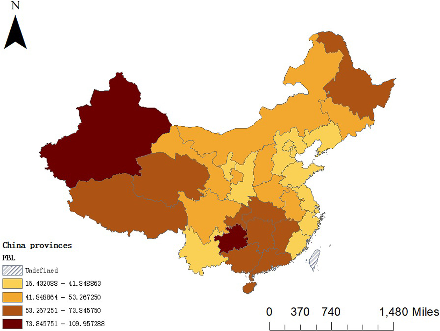
Fig. 1. Distribution of mean incidence of pulmonary tuberculosis in China during 2008–2015.
IPT in China during 2008–2015
In Fig. 2, the blue line denotes the IPT and the brown line denotes the number of persons with pulmonary tuberculosis. It can be seen that the IPT and the number of persons with pulmonary tuberculosis are roughly divided into two stages: from 2008 to 2011 and from 2012 to 2015. It can be seen that the incidence rate in the first stage shows a rapid decrease trend, while the incidence rate in the second stage shows a slow decrease trend. The trend of IPT and number of persons with pulmonary tuberculosis are nearly the same.
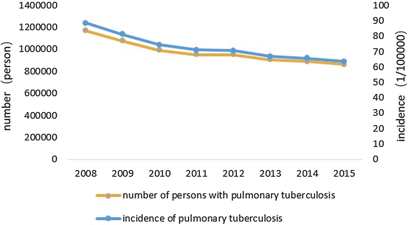
Fig. 2. Incidence of pulmonary tuberculosis and number of persons with pulmonary tuberculosis in China during 2008–2015.
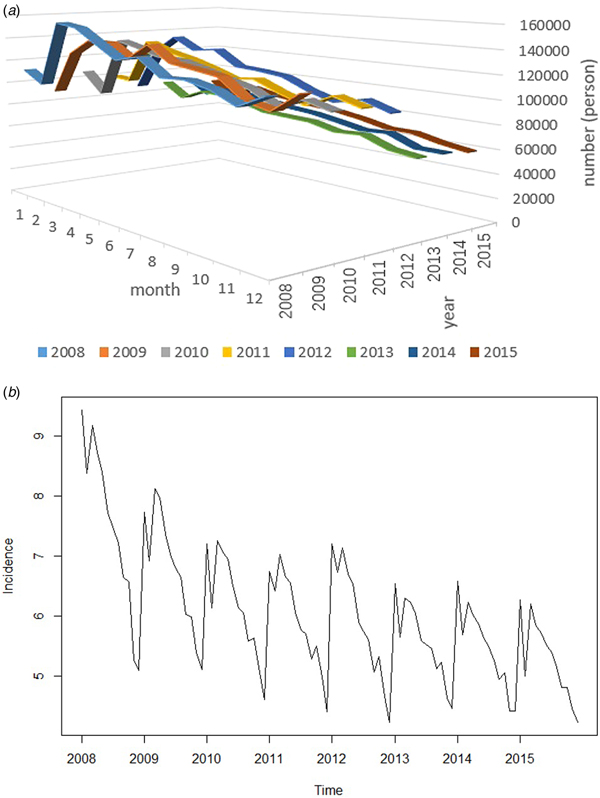
In Fig. 3a, from the seasonal changes, the IPT is lower in winter, higher in spring. Summer and fall showed a downward trend in volatility. From the year series, there are slight fluctuations. The overall trend is decreasing year by year. In Fig. 3b, the IPT has a decreasing trend and there is a cycle phenomenon.

Fig. 3. Time trend. (a) Number of persons with pulmonary tuberculosis in 12 months during 2008–2015. (b) Time series of incidence of pulmonary tuberculosis during 2008–2015.
Local spatial autocorrelation analysis
Since there are missing data and we only have complete data for 2014, we analyse the IPT in 2014 as an example.
Figure 4 shows that in 2014, there are three provinces with statistically significant (P <0.05) in HH (High High) region, including Xinjiang, Tibet and Qinghai. It indicates that the IPT in these provinces is high and the IPT in neighbouring provinces is still high. There are three provinces with statistical significance (P <0.05) in LL (Low Low) region, including Hebei, Beijing and Jiangsu. It indicates that the IPT in these provinces is low and the IPT in the neighbouring provinces is also low. There are two provinces with statistical significance (P <0.05) in LH (Low High) region, including Sichuan and Yunnan. It indicates that the IPT in these provinces is low, but the IPT in the neighbouring provinces is high. There are no statistically significant provinces in HL (High Low) region, indicating that there is no province with a high IPT having neighbouring provinces with a low IPT.

Fig. 4. Results of local Moran index visualisation analysis in 2014.
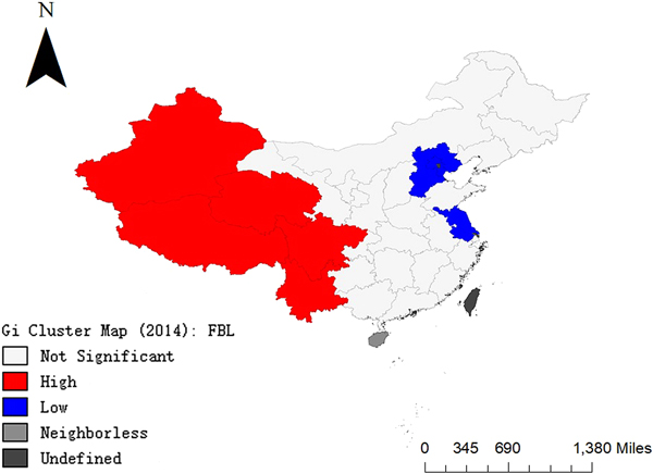
In Fig. 5, Xinjiang, Tibet, Qinghai, Sichuan and Yunnan are clustered areas with high IPT. Hebei, Beijing and Jiangsu are clustered areas with low IPT. In Fig. 6, hot spots (high incidence aggregation areas) are concentrated in the western part of China and cold spots (low incidence aggregation areas) are concentrated in the eastern part of China.

Fig. 5. Results of local G coefficient visualisation analysis in 2014.
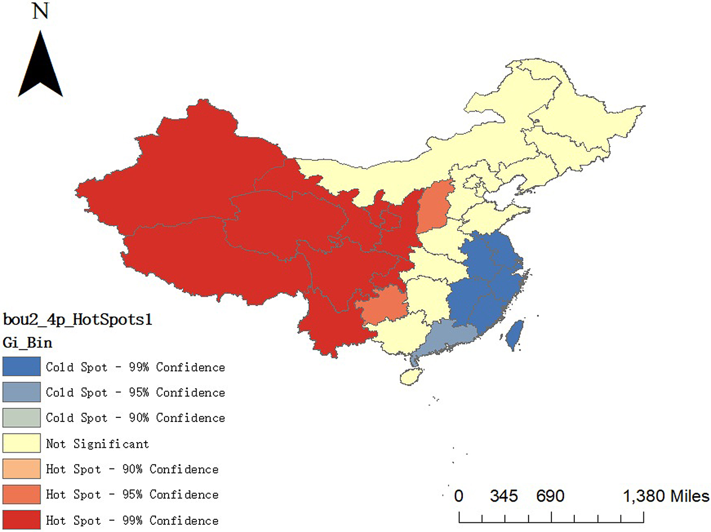
Fig. 6. Results of the hot and cold spot areas in 2014.
Analysis of influencing factors
We find that P = 0.000 <0.05, through Bartlett's Test of Sphericity. Therefore, there are multi-collinearity between influencing factors. We extract four common factors through factor analysis; use factor rotation to get the meaning of the four factors and then name the four factors. Table 1 shows the rotated component matrix. From Table 1, we can see that the first common factor reflects more information about HCL, HT, PGDP, UP, HS and PD. The second common factor reflects more information about CHSC, SWE and PTV. The third common factor reflects more information about the negative of IAIDS and ASS. The fourth common factor reflects more information about BMI and PM. Therefore, the first common factor reflects more information about the economic factor, the second common factor reflects the social service factor, the third common factor reflects the personal factor and the fourth common factor reflects more information about PM and the number of beds in medical institutions. The cumulative variance contribution rate of the four common factors reaches 76.575%. Next, we use these four-factor scores as independent variables to build models.
Table 1. Rotated component matrix

In order to get the impact of these four common factors, Spatial Lag Model was used in this research.
Table 2 shows that C1, C2, C3 are significant except regional C4 when the significance level is 0.05. The IPT in 2014 was negatively correlated with C1, C2 and C3. It indicates that the IPT is high in economically underdeveloped areas. The IPT is high in areas with poor social services. The IPT is high in areas with low average smoking ages. Additionally, the IPT is high in areas with high AIDS prevalence.
Table 2. Regression results of our model for the incidence of pulmonary tuberculosis in 2014

In order to compare the regression effects of Classical Regression Model, Spatial Error Model and Spatial Lag Model, we used three models to regress separately and obtained the following results:
As can be seen from Table 3, the values of AIC and SC of Spatial Lag Model are all smaller than that in Classical Regression Model and Spatial Error Model. The values of R 2 and log L of Spatial Lag Model are all bigger than that in Classical Regression Model and Spatial Error Model. It means that the Spatial Lag Model fits better than two others. In Table 4, Spatial Lag Model passed the Robust LM tests with P < 0.05 while Spatial Error Model failed. Therefore, Spatial Lag Model has a better interpretation.
Table 3. Comparison of regression results of three models

a Spatial error model.
b Classical regression model.
c Spatial lag model.
d Log likelihood.
e Akaike information criterion.
f Schwarz criterion.
Table 4. Results of the spatial dependence test for the incidence of pulmonary tuberculosis in 2014

Discussions and conclusions
In this research, we analysed the IPT during 2008–2015 in terms of space, time and influencing factors comprehensively.
There is a significant difference in the incidence of tuberculosis in various provinces, which is characterised by low in the east and high in the west. It is related to the unbalanced economic development in some ways. The economic development in the east is higher than that in the west, making the entire system of medical care and prevention in the east more complete than in the west. Studies [Reference Hou21] show that people in areas with economic underdevelopment are more likely to get tuberculosis due to AIDS, drug use, application of immunosuppressive agents, alcoholism and poverty.
In particular, studies [Reference Edelson22, Reference Mohr23] have shown that public transportation is closely related to the spread of Mycobacterium tuberculosis. It is also related to the incidence of tuberculosis. The terrain in the western region is complex, so the traffic is inconvenient, while the eastern region is plain and the transportation is more convenient.
At the same time, the overall quality of the population in the east is higher than that in the west and their awareness of prevention and treatment is stronger than that of the western residents [Reference Zhu24]. There are more AIDS patients in the western region. Tuberculosis is one of the most common opportunistic infections in AIDS patients. The two diseases affect each other and cause each other. AIDS patients have 30–50 times more likely to have tuberculosis than normal people [Reference Li25]. Therefore, the incidence of tuberculosis is high in the west and low in the east.
From the analysis results, we can see that the incidence of tuberculosis is seasonal. The formation of the peak incidence of tuberculosis in the population has been analysed by Zhang et al. [Reference Zhang26]. There are two main reasons. On the one hand, the spread of Mycobacterium tuberculosis in the population leads to an increase in the incidence of recent transmission. On the other hand, the immunity decreases and the incidence of latent infections in the population have increased. According to the survey, the peak incidence of tuberculosis is in spring, during the Chinese Lunar New Year period and the population movement is large, so that there are more opportunities for tuberculosis transmission, increasing the chance of infection of susceptible people [Reference Wang27]. The peak period in summer is mainly due to the dryness of the air, the decrease of respiratory mucosal resistance and the cold weather of the air in the winter. The infected tuberculosis is in the incubation period and has a certain time from the onset to the diagnosis. The diagnosis was delayed, which led to the peak incidence of the report in spring or summer. Fundamentally speaking, the seasonal difference in the incidence is due to geographical and climatic reasons. The weather varies from season to season and the human immunity will be different.
The reason for the decrease in the IPT in recent years may be due to the fact that the state has always attached importance to the prevention and treatment of tuberculosis. The State Council issued the National Tuberculosis Prevention and Control Plan (2001–2010) in 2001 [Reference Yu28]. The scientific improvement of disease diagnosis and treatment methods, the disease screening rate and the increasing awareness rate of core information for tuberculosis prevention and control among the people have a great relationship with the decrease in the incidence of tuberculosis.
We have found the seasonality of tuberculosis incidence. This characteristic can remind residents to prepare for the prevention of pulmonary tuberculosis in advance. It can also remind the hospital to purchase tuberculosis-related drugs in advance. Additionally, it can remind the government to introduce relevant policies to prevent tuberculosis.
Through the spatial clustering of pulmonary tuberculosis, we can see which areas have a high IPT and which areas have a low IPT. At the same time, we need to focus on strengthening treatment in areas with high IPT and prevention of tuberculosis in high incidence areas spreading to surrounding areas.
Through quantitative analysis, we analysed factors influencing the IPT. According to our conclusion, the government can improve the IPT by improving the level of economic development and regulating social services. Individuals can reduce the IPT by reducing smoking and the likelihood of being infected with AIDS.
In sum, our model has two highlights: (a) Compared with the other two models, Spatial Lag Model can fit the data better. The values of AIC and SC of Spatial Lag Model are all smaller and the values of R 2 and log L are all bigger than those in the other two models. (b) Compared with the Spatial Error Model, our model is more significant in the spatial dependence test for the IPT.
There are still some limitations to our model: (a) It ignores whether there are spillover effects in one area to a certain extent. (b) There are only 13 explaining variables in this research. In fact, there are a lot of influencing factors. Those are what the future work needs to further improve. From the perspective of space, the IPT varies significantly among regions in China. The overall situation is that the eastern part has low incidence and the western part has a high incidence. From the perspective of time, the IPT has been slowly decreasing in recent years. The IPT has certain seasonal characteristics: lower in winter, higher in spring and decreasing unsteadily in summer and autumn.
Financial support
This research was funded by National Natural Science Foundation of China (No.11471053), Key Laboratory of Universal Wireless Communications (KFKT-2015103) and Student's Platform for Innovation and Entrepreneurship Training Program of Beijing University of Posts and Telecommunications: 201807003.
Conflict of interest
The authors declare no conflict of interest.


 Open access