


Introduction
In October 2015, the International Agency for Research on Cancer (IARC), a body of the World Health Organization, released a report classifying processed meat as a type 1 carcinogen. Footnote 1 The announcement immediately led to panicked headlines, such as “The Great Bacon Freakout,” “Bacon Causes Cancer,” and “The End of the Road for Bacon.” Despite the high level of national attention given to the IARC report, it remains unclear what, if any, impact the report had on sales of processed meat products.
To the extent the information in the IARC report dampened consumer demand, one would expect lower prices and purchase volumes as a result. In this paper, we utilize retail scanner data to investigate whether and to what extent the IARC report indeed led to these outcomes. A challenge in identifying the effects of the report is that the information was widely distributed and may have affected multiple meat products, making it difficult to construct a counterfactual prediction of the trends in processed meat prices and purchases that would have occurred absent the IARC information. To overcome these challenges, we employ a synthetic control method (SCM) to empirically identify products, pre-IARC release, that co-move with processed meat prices and purchases.
Empirical evidence of market response to the IARC report is limited. Related studies exploring the effect of health information on meat demand finds various market responses to different information. Traditional studies have estimated structural demand models, and have included counts of media or scientific reports about health consequences of meat consumption. Some studies find such health information shifts meat demand (Brown and Schrader Reference Brown and Schrader1990; Kinnucan et al. Reference Kinnucan, Xiao, Hsia and Jackson1997; Tonsor, Mintert, and Schroeder Reference Tonsor, Mintert and Schroeder2010; Piggott and Marsh Reference Piggott and Marsh2004), while others find that impact depends on type of information. For instance, high risk events, such as food scares, tend to have higher impacts on food consumption than other types of information (e.g. Liu, Lien, and Asche Reference Liu, Lien and Asche2016; Rieger, Kuhlgatz, and Anders Reference Rieger, Kuhlgatz and Anders2016). The impact of health information is found to be relatively small compared with other effects such as income, price, and tastiness of food. For instance, Malone and Lusk (Reference Malone and Lusk2017) find health perceptions affect consumers’ willingness to pay for meat products, but the effect is much smaller than perceptions of tastiness. Marsh, Schroeder, and Mintert (Reference Marsh, Schroeder and Mintert2004) find that although meat recall events significantly impact demand, newspaper reports do not. Yadavalli and Jones (Reference Yadavalli and Jones2014) observe significant effects of media broadcasting on meat demand, but the effects are temporary and disappeared within a week. Moreover, when both positive and negative information is present at the same time, the combination of the impacts is muted (Tonsor, Mintert, and Schroeder Reference Tonsor, Mintert and Schroeder2010), with research often suggesting that negative information is more impactful than positive information (Chang and Kinnucan Reference Chang and Kinnucan1991). Thus, much remains to be learned about the impact of health information on meat demand generally, and about the impact of the IARC report on processed meat consumption specifically.
The IARC report concluded that regular consumption of processed meat increases risk of colorectal cancer Footnote 2 . Consumers exposed to this information may interpret it to imply processed meat is a health threat, leading to reduction in willingness to pay for processed meat products. Likewise, firms (packers or retailers) might adjust prices in response to the demand change. In this paper, we test for these hypothesized shifts via inspecting the changes in prices, quantities, and expenditures of selected processed meat products before and after the release of the IARC report relative to a synthetic control.
We advance the literature from several perspectives. To our knowledge, there has been little work examining the effect of the IARC report on the prices or sales of processed meat products despite the wide media coverage of the event at the time it was released. Even though many studies have explored the impacts of health information on meat demand, none of them has investigated the economic outcome of the IARC report. In addition, existing studies showing adverse relationships between meat demand and negative health information (such as fat, cholesterol, etc.) have mainly use structural demand estimation approaches that incorporate media indices as one determinant of consumer demand (e.g. Kinnucan et al. Reference Kinnucan, Xiao, Hsia and Jackson1997; Brown and Schrader Reference Brown and Schrader1990; Tonsor, Mintert, and Schroeder Reference Tonsor, Mintert and Schroeder2010). Instead of using a structural approach, we conduct an intervention analysis and estimate the relative changes in economic outcomes (price, sales, and expenditures) after the IARC report was released. We utilize the SCM for intervention analysis using weekly transaction grocery scanner data. To the best of our knowledge, this method has not been applied to this topic to date.
We construct a synthetic control group, which consists of food products that are not (or at least are plausibly weak) substitutes for processed meat. The synthetic control is a convex combination of these products’ prices, quantities, or expenditures, where each potential control product is assigned a different weight. We estimate the weight by minimizing the difference between the synthetic control product and target product price, quantity, or expenditure prior to the report release. The constructed control product is, thus, designed to have parallel trends with the treatment product pre-intervention. By comparing the simulated counterfactual outcomes (i.e., the constructed synthetic control) with observed outcomes, we are able to measure the effect of the IARC report on prices, sales and expenditures for selected processed meat products.
Because the IARC report content was widely accessible and reported globally, conventional difference-in-difference methods would likely produce biased results because, for example, it would be virtually impossible to find a control location not affected by the information. The SCM sidesteps this problem and uses a combination of candidate product controls instead. We use Nielsen retail scanner data to determine the effect of the IARC report on selected processed meat products. This data contains weekly information regarding sales, price, and revenue for processed meat categories as well as categories that are included in the synthetic control group. We use the data from 2014 to 2016, which includes approximately one year of data before and one year of data after IARC report released date. The post-IARC time period is long enough to determine if any impact exists and how long it lasts.
In addition to estimating the information effect on selected processed meat markets, we check whether our results are spurious by conducting placebo tests using products within the synthetic control group. Specifically we estimate the change for each presumably unaffected (nonprocessed meat) product as if these were influenced by the IARC information. By ranking the magnitude of estimated effects for all products, we obtain statistical inference as to whether price/sales/expenditure of target products have changed significantly after the IARC report was released. Our final results indicate a significant reduction in price and expenditures on bacon. At the same time, there was a significant increase in quantity of beef purchased.
In the following, we introduce the SCM. In the next section, we describe the data. We discuss placebo tests in the “Placebo test methods” section and describe our estimation results in the “Results” section. In the “Results” section, we also discuss what the estimated price, quantity, and revenue changes imply about demand and supply shifts. We end with a conclusion.
Synthetic Control Method
To investigate the impact of the IARC report, we use the synthetic control algorithm developed by Abadie and Gardeazabal (Reference Abadie and Gardeazabal2003) and Abadie, Diamond, and Hainmueller (Reference Abadie, Diamond and Hainmueller2010). This method computes a synthetic control group that simulates counterfactual outcomes as if the IARC report were absent. This computed control group ensures the satisfaction of parallel trend between treated and control variables before intervention, as it calculates weights for products in the product candidate pool that minimizes the difference between control and treatment products. Instead of looking for one control product, this method helps to construct an appropriate comparison unit using a convex combination of many candidate products.
In practice, we assume $j = 1,2, \ldots ,J$
are the products of interest that are affected by the report, and we take these products as treated products in our analysis. We assume
$j = 1,2, \ldots ,J$
are the products of interest that are affected by the report, and we take these products as treated products in our analysis. We assume $k = 1,2, \ldots ,K$
are products that are not affected by the IARC report; we use the K candidate products to compute a synthetic control. Essentially, we make use of these candidate products to construct a new product that simulates the cases where the product of interest was not affected by intervention.
$k = 1,2, \ldots ,K$
are products that are not affected by the IARC report; we use the K candidate products to compute a synthetic control. Essentially, we make use of these candidate products to construct a new product that simulates the cases where the product of interest was not affected by intervention.
Suppose we have a balanced sample, which contains weekly price, sales, and revenue records of each product in our treatment and control group. The sample has ${T'}$
periods in total, pre-intervention periods last from
${T'}$
periods in total, pre-intervention periods last from $t = 1$
to
$t = 1$
to $T,T \lt{T'}$
, and post-intervention periods are from
$T,T \lt{T'}$
, and post-intervention periods are from $t = T + 1$
to
$t = T + 1$
to ${T'}$
. To distinguish between the two, we use t to denote pre-intervention periods and
${T'}$
. To distinguish between the two, we use t to denote pre-intervention periods and ${t'}$
denotes post-intervention periods.
${t'}$
denotes post-intervention periods.
We construct a synthetic control product for each treated product and variable that is presumably affected by the IARC report. We assign a weight to each candidate product in the control group, and these weights are denoted as $W = [{w_1},{w_2}, \ldots ,{w_k}]$
. The sum of weights equals one (
$W = [{w_1},{w_2}, \ldots ,{w_k}]$
. The sum of weights equals one ( $0 \le {w_k} \le 1$
and
$0 \le {w_k} \le 1$
and $\sum\nolimits_{k = 1}^K {w_k} = 1$
). In this way, we construct a synthetic control product as a convex combination of candidate products by selecting an appropriate weight vector W. The best synthetic control should well represent the trends of treated products during the pre-intervention periods. Based on this objective, we select W that minimizes the distance between the outcomes of synthetic control product and treated product during pre-intervention periods.
$\sum\nolimits_{k = 1}^K {w_k} = 1$
). In this way, we construct a synthetic control product as a convex combination of candidate products by selecting an appropriate weight vector W. The best synthetic control should well represent the trends of treated products during the pre-intervention periods. Based on this objective, we select W that minimizes the distance between the outcomes of synthetic control product and treated product during pre-intervention periods.
Suppose ${Y_{jt}}$
is the outcome variable (i.e., price, volume purchased, or expenditures) of each treated product during pre-intervention periods, and
${Y_{jt}}$
is the outcome variable (i.e., price, volume purchased, or expenditures) of each treated product during pre-intervention periods, and ${Y_{kt}}$
is the outcome variable of each product in the control group. The difference between treated and synthetic control product is calculated through
${Y_{kt}}$
is the outcome variable of each product in the control group. The difference between treated and synthetic control product is calculated through ${Y_{jt}} - {Y_{kt}}W$
, where
${Y_{jt}} - {Y_{kt}}W$
, where ${Y_{jt}}$
is a
${Y_{jt}}$
is a $T \times 1$
vector,
$T \times 1$
vector, ${Y_{kt}}$
is
${Y_{kt}}$
is $T \times K$
vector and W is a
$T \times K$
vector and W is a $K \times 1$
vector. We choose
$K \times 1$
vector. We choose ${W^*}$
that minimizes the absolute value of the difference. We solve the problem
${W^*}$
that minimizes the absolute value of the difference. We solve the problem
 $${W^*} = {A_W}({Y_{jt}} - {Y_{kt}}W)'V({Y_{jt}} - {Y_{kt}}W)$$
Where ${V_k}$
is the
${V_k}$
is the $K \times K$
weight matrix that determines the importance of each product within the synthetic control group. In general,
$K \times K$
weight matrix that determines the importance of each product within the synthetic control group. In general, ${V_k}$
assigns higher weights to products with greater power in predicting price/sales/revenue of the treated product. The prediction power of each product can be estimated using a cross-validation method and assign weights accordingly. In our analysis, we assume a uniform prediction power across products within the candidate product pool, so
${V_k}$
assigns higher weights to products with greater power in predicting price/sales/revenue of the treated product. The prediction power of each product can be estimated using a cross-validation method and assign weights accordingly. In our analysis, we assume a uniform prediction power across products within the candidate product pool, so ${V_k}$
is a
${V_k}$
is a $k \times k$
matrix with all diagonal elements equal to 1.
$k \times k$
matrix with all diagonal elements equal to 1.
Data
In our analysis, we use weekly Nielsen retail scanner data. The data we use runs from January 2014 to December 2016. This data set has been widely used in food market analysis and is generated from a point-of-sale system that collects information from more than 35,000 retail stores belonging to over 90 chains in the United States. This data contains representative stores with store types including grocery, drug store, mass merchandiser, convenience stores, etc. Stores in this data set cover over half of the sales volume of grocery and drug stores and over 30% of the sales volume of mass merchandisers in the USA. The retail scanner data contains weekly transaction information of products at the Universal Product Code (UPC) level for each sampled store. Every week, the participating stores report sale units, prices, and other product features (e.g. display, promotion, etc.). In total, this data contains 2.6 million UPCs, including food products, nonfood groceries, and health and beauty products.
In this study, we focus on three processed meat items: bacon, sausage, and ham. These are processed meat items that consumers might plausibly link to the information in the IARC report (i.e., these are “treated” products). Because each of these categories consists of products of different type, flavor and packaging, we aggregate within each category and calculate average unit price, total sale volume, and revenue/expenditure for each category and each week.
Our analysis does not estimate impacts of the IARC report on all possible processed meat products, as we do not study items such as hot dogs, canned meat, and lunch meats. However, in the pork sector, sales of bacon, sausage, and ham are substantially higher than those of other processed meats such as frankfurters, bologna, etc. If the IARC report impacts processed meat demand, one would expect it to affect the major processed meat categories of bacon, sausage, and ham; if these key processed pork items are not affected by the IARC report, one must question whether the report had a substantive impact on overall processed meat demand. Nonetheless, our findings may or may not apply to other processed pork items.
As previously indicated, a challenge rests in identifying a control set of products or locations that: (1) are not affected by the IARC report but; (2) are good predictors of processed meat purchases. We select a group of food products that are plausibly independent of or are weak substitutes for processed meat. In addition, we select products that are most frequently purchased by consumers to ensure we have sufficient data points (for each week, we need price, sales, and revenue for each category at each store). We use these products to construct a synthetic control group as described in the previous section. As indicated, the method thus ensures that the parallel trend assumption is maintained prior to the report release. The key assumption is that the relationship between price/sales/purchase of the synthetic control and target product would have continued had the IARC report not been released.
To construct the control, we picked 50 food and food-related categories with top purchase frequencies within all the 1,100 categories in the Nielsen data. The categories that are included in our synthetic control group include apples, baby food, dry beans, broccoli, butter, cake, candy, carrots, celery, cereal, cheese, chili sauce, corn, corn chip, eggs, entree, frozen fruit, green bean, ice cream, jams, macaroni, Mexican sauce, milk, nuts, orange juice, oranges, pasta, peanut butter, peppers, pizza, popcorn, pork rinds, potatoes, pretzels, raisins, refrigerated fruit, rice mix, rice, salt, soup, tea, tomatoes, vinegar, and yogurt.
For each category, in both the control and treatment group, we aggregate outcomes into weekly data at national level. Aggregate prices are calculated by weighting by store sales volume. That is, rather than summing unit prices across stores and dividing by the number of stores ( ${p_{jt}} = {1 \over N} \times \sum\nolimits_{i = 1}^N {{p_{ijt}}} $
), we weight the unit price of each store by the ratio of store sales to total sales of all stores in the USA (in equation 2). Therefore, stores with higher weekly sales have higher weights in determining the average product price in the USA. This helps ensure we are utilizing nationally representative average prices paid by consumers.
${p_{jt}} = {1 \over N} \times \sum\nolimits_{i = 1}^N {{p_{ijt}}} $
), we weight the unit price of each store by the ratio of store sales to total sales of all stores in the USA (in equation 2). Therefore, stores with higher weekly sales have higher weights in determining the average product price in the USA. This helps ensure we are utilizing nationally representative average prices paid by consumers.
The calculation is as follows
 $${p_{jt}} = \sum\limits_{i = 1}^N {{p_{ijt}}} \times {{{q_{ijt}}} \over {{Q_{jt}},}}$$
where
 $${Q_{jt}} = \sum\limits_{i = 1}^N {q_{ijt}}.$$
Here, ${p_{jt}}$
is weighted average unit price of product j at week t.
${p_{jt}}$
is weighted average unit price of product j at week t. ${p_{ijt}}$
denotes the unit price of product j in week t at store i.
${p_{ijt}}$
denotes the unit price of product j in week t at store i. ${q_{ijt}}$
denotes total unit sales of product j at store i in week t,
${q_{ijt}}$
denotes total unit sales of product j at store i in week t, ${Q_{jt}}$
is the total sales of product j at week t across all stores. The way we calculate
${Q_{jt}}$
is the total sales of product j at week t across all stores. The way we calculate ${p_{jt}}$
is equivalent to summing revenues and then dividing total sales across all stores.
${p_{jt}}$
is equivalent to summing revenues and then dividing total sales across all stores.
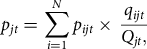
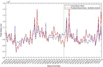
Figures 1–6 illustrate the constructed weekly prices, sales, and revenues for each processed meat product before and after the IARC report release date. The red lines represent processed meat products and blue line denotes counterfactuals, which use the synthetic control to simulate the outcome variables absent the intervention. Figures 1 and 2 describe the actual and simulated bacon price and quantity sold. Figure 1 shows a remarkable dip in simulated bacon price immediately following the IARC report release. The periods during which bacon price fell overlap with holidays such as Thanksgiving and Christmas. The observed price dip might be partially caused by the price promotions during holidays. However, it should be noted that weights were assigned to control products in the SCM that would have also matched the usual seasonal trends in product prices in the pre-intervention period.
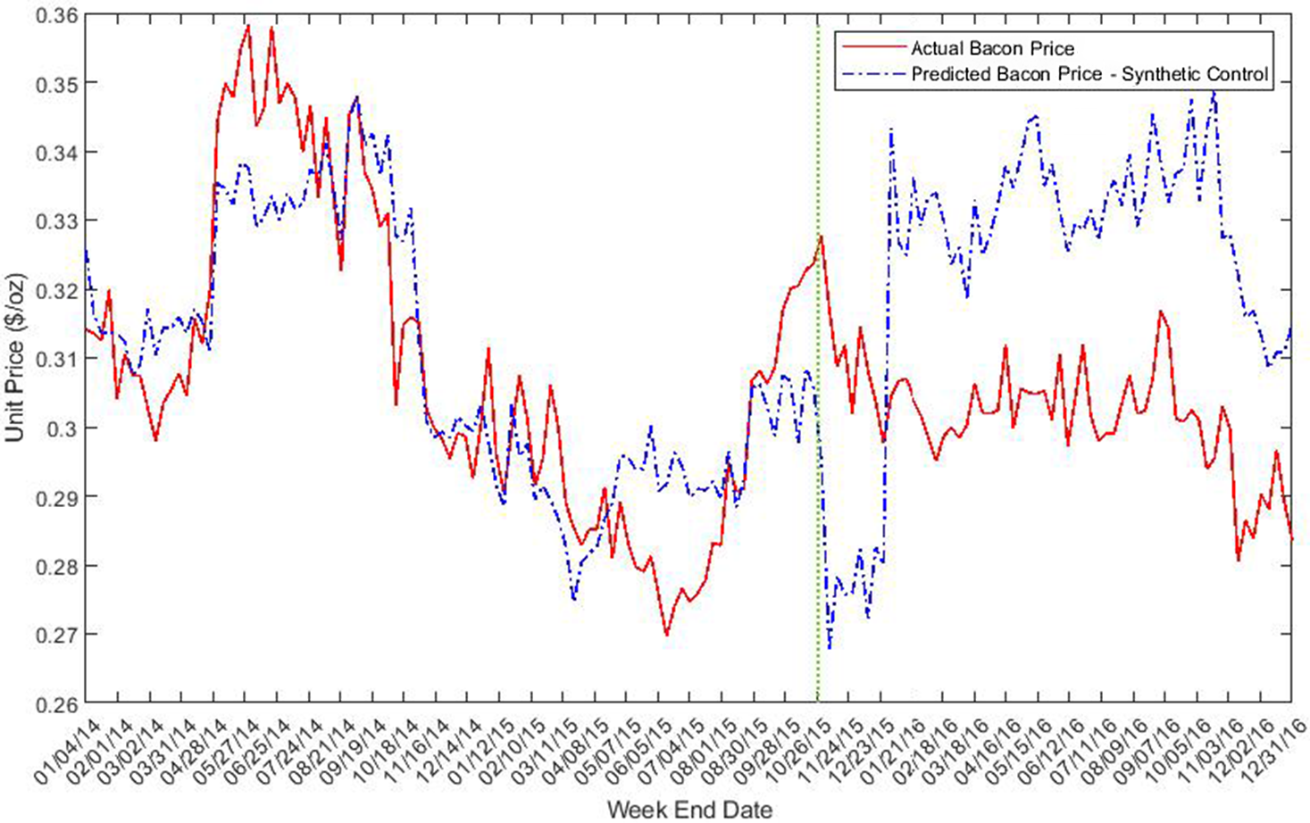
Figure 1. Unit price of bacon ($/oz).
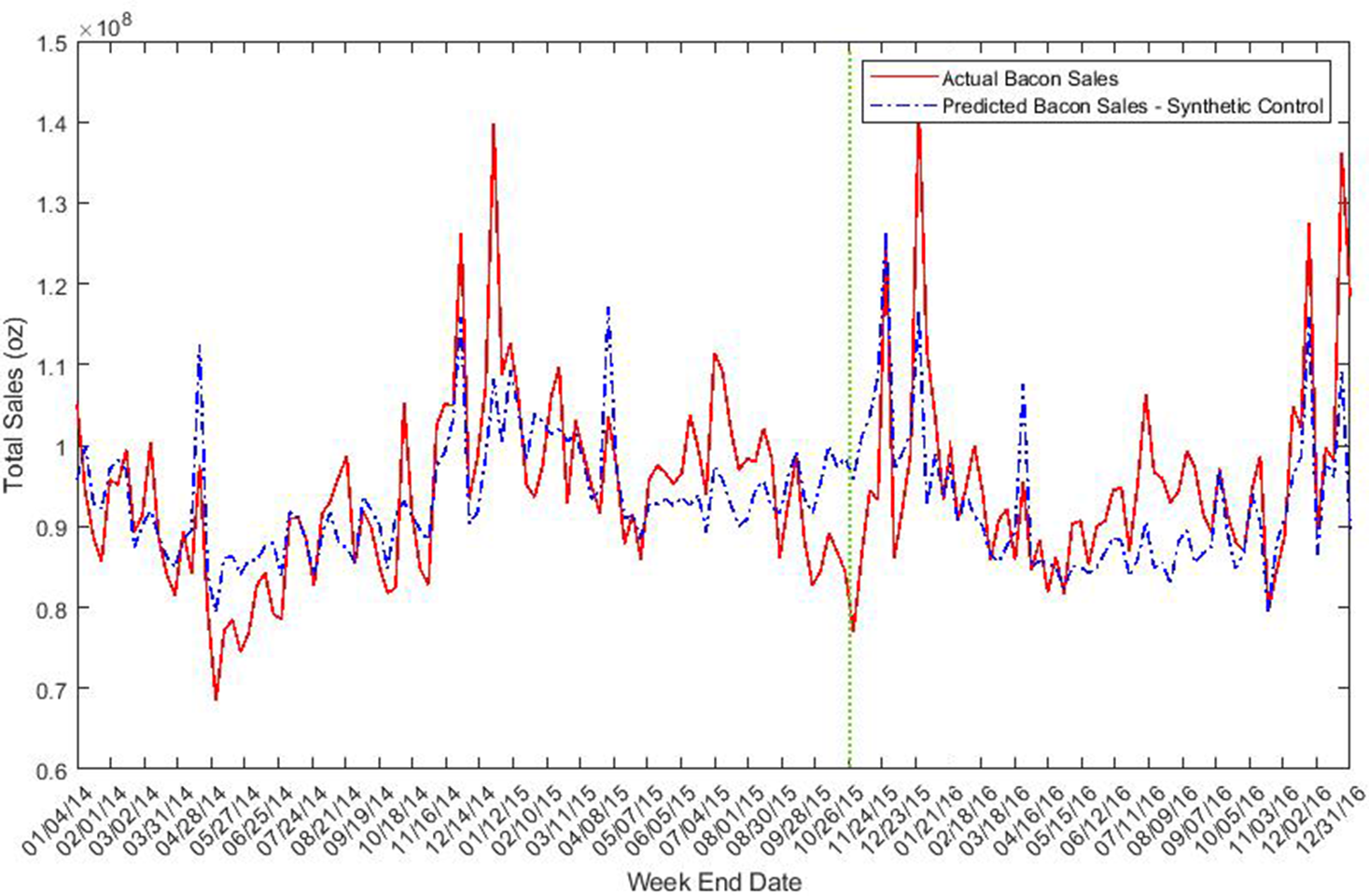
Figure 2. Total sales of bacon (oz).
After the holidays (the week after Dec 25), the simulated control price increases dramatically and ends up with a higher price relative to the actual bacon price. That is, the actual bacon price failed to return to its normal level after the holiday season, which is likely the result of the IARC report impact. Unlike price, the deviation between the actual and simulated bacon sales quantity is not noticeable from the plot.
Figure 3 illustrates the trends in sausage price. We observe a good fit between actual and simulated price of sausage during pre-intervention periods. A remarkable divergence is observed right after the intervention, with actual sausage price below the synthetic control. There is also a tendency for quantity of sausage sold to increase in the post-intervention period relative to the synthetic control (see Figure 4). Figure 5 reveals only slight differences between real and simulated prices for ham. The quantity of ham sold was generally lower in the post-IARC report period relative to the counterfactual synthetic control quantity (see Figure 6).
Figure 3. Unit price of sausage ($/oz).
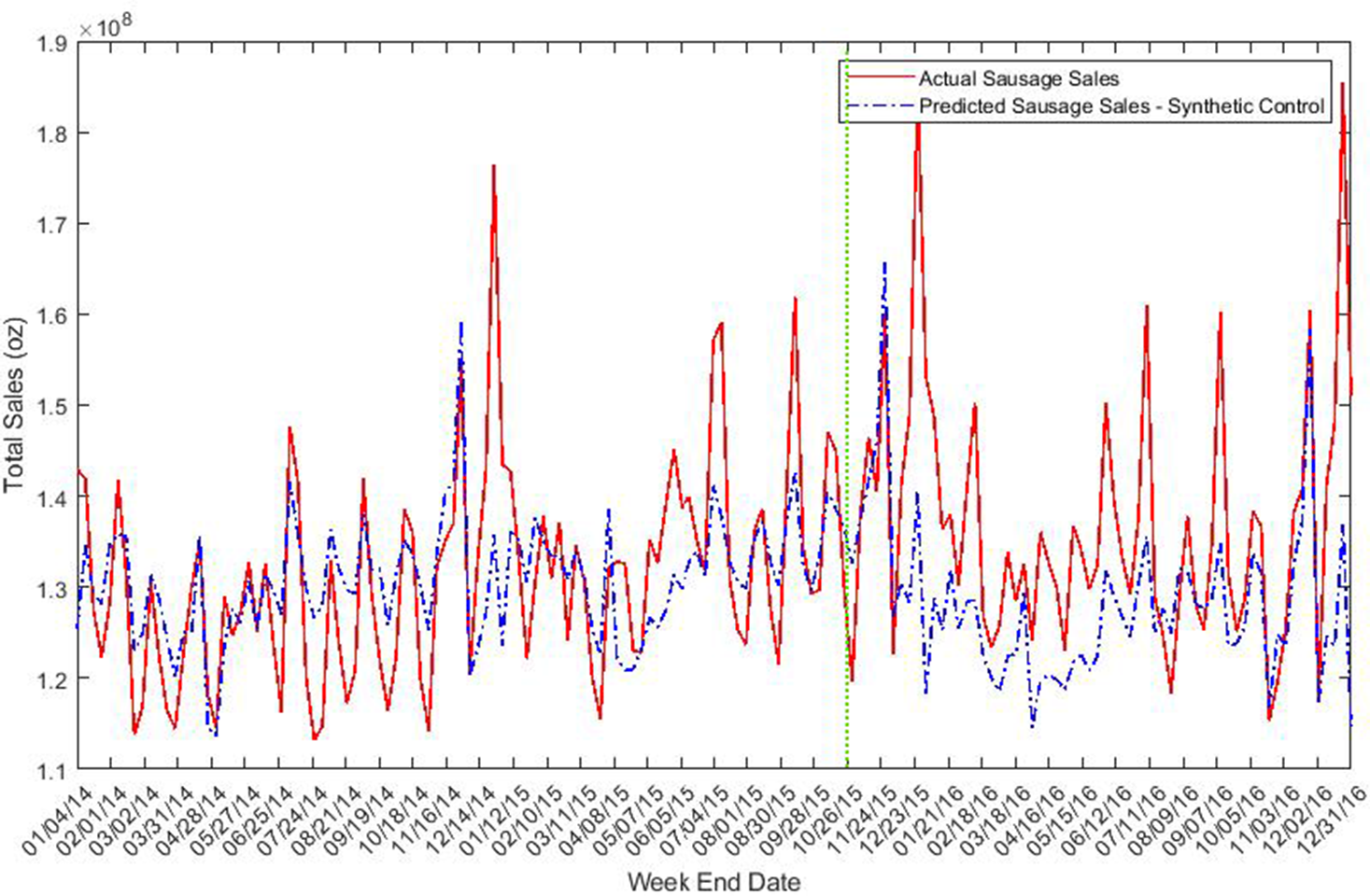
Figure 4. Total sales of sausage (oz).
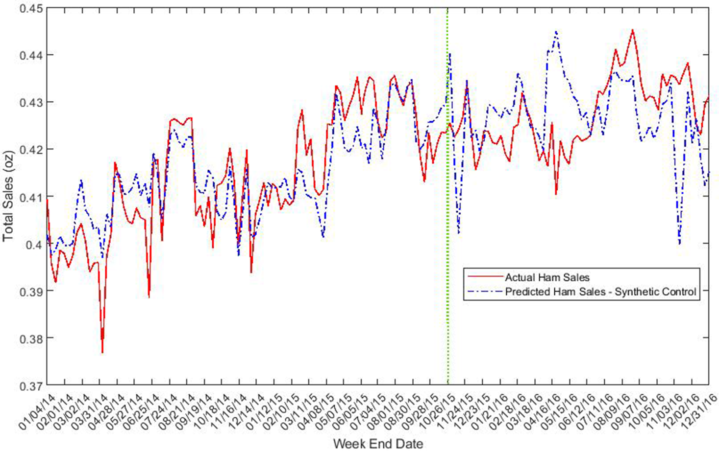
Figure 5. Unit price of ham ($/oz).
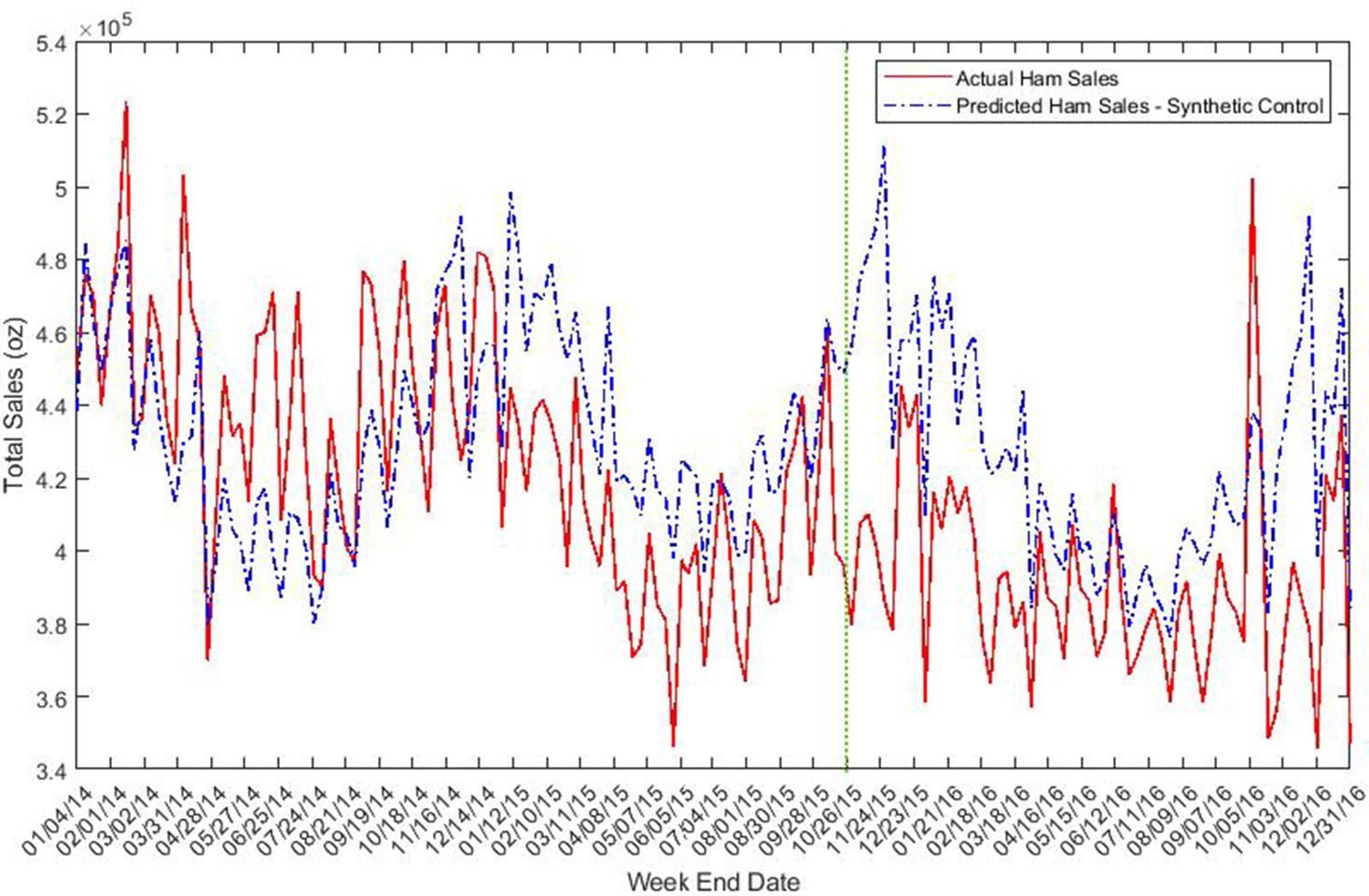
Figure 6. Total sales of ham (oz).
Placebo test methods
In addition to estimating the intervention effect on each treated product, we conduct placebo tests to determine the statistical significance of the estimated effects. To achieve this goal, we calculate the probability that the effects for target products are larger than for products where intervention is presumed not to exist. In this way, we provide statistical evidence that the changes we find (in price and sales) are caused by the IARC report rather than some random factors. In this process, we use all the candidate products in the control group as placebos to estimate the price and sales change for each of the products.
We applied the same approach as Abadie and Gardeazabal (Reference Abadie and Gardeazabal2003), Bertrand, Duflo, and Mullainathan (Reference Bertrand, Duflo and Mullainathan2004) and Abadie, Diamond, and Hainmueller (Reference Abadie, Diamond and Hainmueller2010) to conduct the placebo tests. We calculate the intervention effect by applying the synthetic control approach (as described in the “Synthetic Control Method” section) to products that were not supposed to be affected by the IARC report. This is to check if the effect estimated using these placebo products is larger than the effect estimated for the processed meat category. We use 90% as threshold. If the treated product (processed meat) has a larger influence (i.e., bigger changes in price, sales, or revenue) than 90% of placebo products, we conclude that the IARC report has a significant impact on processed meat outcomes. Otherwise, we conclude that the influence is not significantly different than changes that would have arisen from chance (or not significantly different from having no effect).
When measuring the changes after intervention, we make some adjustments in calculating the intervention effect. This adjustment is based on the observation that for some placebo products the simulated outcome of constructed synthetic control products is not close to the observed value in pre-intervention period. To incorporate the difference between actual and simulated outcomes during pre-intervention periods, we adjust post-intervention effect estimates by subtracting the mean difference in pre-intervention periods. We denote the difference as $D = {Y_a} - {Y_s}$
, where
$D = {Y_a} - {Y_s}$
, where ${Y_a}$
denotes the actual value of outcome variables (price, sales and revenue),
${Y_a}$
denotes the actual value of outcome variables (price, sales and revenue), ${Y_s}$
denotes simulated outcomes.
${Y_s}$
denotes simulated outcomes. $D(t \gt I)$
indicates the difference is derived using values from post-intervention periods and
$D(t \gt I)$
indicates the difference is derived using values from post-intervention periods and $\overline D (t \le I)$
denotes mean of difference during pre-intervention.
$\overline D (t \le I)$
denotes mean of difference during pre-intervention.
Specifically,
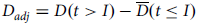 $${D_{adj}} = D(t \gt I) - \overline D (t \le I)$$
We then use ${D_{adj}}$
to measure the information effect instead of D. In this way, we are able improve our estimates by controlling the goodness of fit during pre-intervention periods.
${D_{adj}}$
to measure the information effect instead of D. In this way, we are able improve our estimates by controlling the goodness of fit during pre-intervention periods.
Results
As described in previous sections, we construct the synthetic control product as a convex combination of candidate products in the control group. We use the constructed synthetic control product to simulate the outcome of treated products as if the intervention effect were absent. Comparing the difference between treatment and synthetic control outcomes, we test the effect of health information released in the IARC report on prices, quantity sold, and expenditures/revenue for selected processed meat products: bacon, sausage, and ham.
In this study, we use January 2014 to October 24, 2015 as pre-intervention periods to calculate weights for each candidate product and construct synthetic controls. We use October 24, 2015 to December 2016 as post-intervention periods to check the difference between real and simulated outcome variables to estimate the intervention effect of the report. Our data consist of weekly observations. Because October 24th is the end of the week before the week of the intervention (October 26), we use the week ending in October 24 as threshold to separate pre- and post-intervention periods. This cut-off also makes sense given that more transactions are made at the end of each week (e.g. weekends) instead of at the beginning. The week after October 24 is the first week that is subject to the impact of the IARC report.
Summary statistics for prices, total quantity sales, and expenditures for each of the selected processed meat categories before and after IARC report release date are reported in Table 1. Table 1 indicates unit price, purchase volumes and expenditures are, by construction, nearly the same in treatment and synthetic control group for bacon, sausage and ham categories before the report was released.
Table 1. Summary statistics of price, sale and expenditure of processed meat
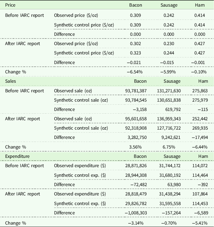
Note: Change % = (difference (after) – difference (before))/synthetic control value (after).
Our result shows that the estimated intervention effect of the IARC report on bacon price is −0.021. This indicates that after the IARC report release date, bacon price decreased by 2.1 cents per ounce on average relative to the counterfactual prediction of what would have happened if the IARC report had not been released. Compared with what would have been the case had the IARC report been absent, bacon price decreased by 6.54% after report release date. At the same time, consumers’ total expenditures on bacon fell by $1 million (3.14%) with quantity purchased increasing by 3.56% per week on average after the IARC report release date, among all the sampled stores in the Nielsen data set.
Similar to bacon, the estimated information effect of the IARC report on sausage price is also negative. The report information resulted in sausage price falling by 1.5 cents per ounce, which is equivalent to a 5.99% price decrease compared to no intervention. Concurrently, weekly sausage sales increased by 9.2 million ounces, or 6.85%, on average among all stores sampled by Nielsen in the USA. Total sausage expenditures fell by $157,264, or −0.1%.
The pattern of price, quantity, and expenditure changes for ham differed from that for bacon and sausage. Whereas bacon and sausage quantities increased following the IARC report, ham quantities fell by 6.44%. The intervention effect on ham price is close to zero but negative (−0.1%). Ham expenditures fell 5.41% after the release date of the IARC report.
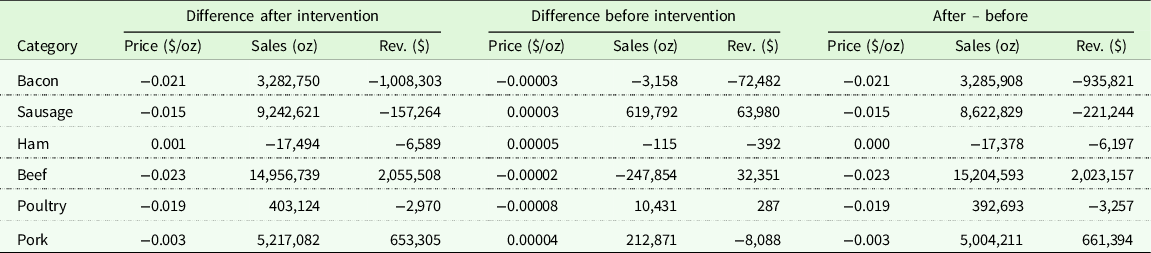
The estimation of intervention effects on each processed meat product is shown in Table 2. The top part of the table repeats what is shown in Table 1, and for comparison, the bottom three rows show impacts on aggregate categories of fresh beef, poultry, and pork. All three fresh product prices fell, and quantities rose, following the release of the IARC report.
Table 2. Information intervention effect on processed meat and fresh meat
To further test if the changes are statistically significant or spurious, we conduct placebo tests as described in the previous section. The nonadjusted and adjusted results of placebo tests are reported in Tables 3 and 4. In these tables, we rank products according to their estimated intervention effects from smallest to largest. The products ranked from 1-6 ( $ \lt 11\% $
) and 48–53 (
$ \lt 11\% $
) and 48–53 ( $ \gt 89\% $
) are viewed as products having significant changes after intervention compared to the placebo products. In addition, we plot the price and expenditure changes for all processed meat products in Figures 7 to 12.
$ \gt 89\% $
) are viewed as products having significant changes after intervention compared to the placebo products. In addition, we plot the price and expenditure changes for all processed meat products in Figures 7 to 12.
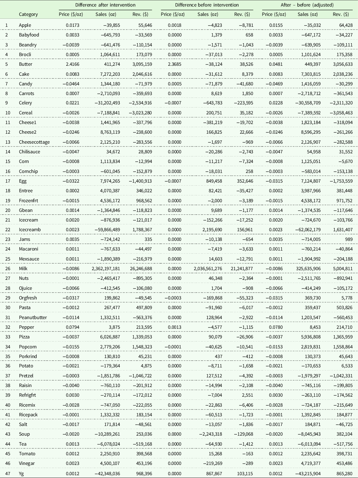
Table 3. Result of placebo test ranked by effect magnitude
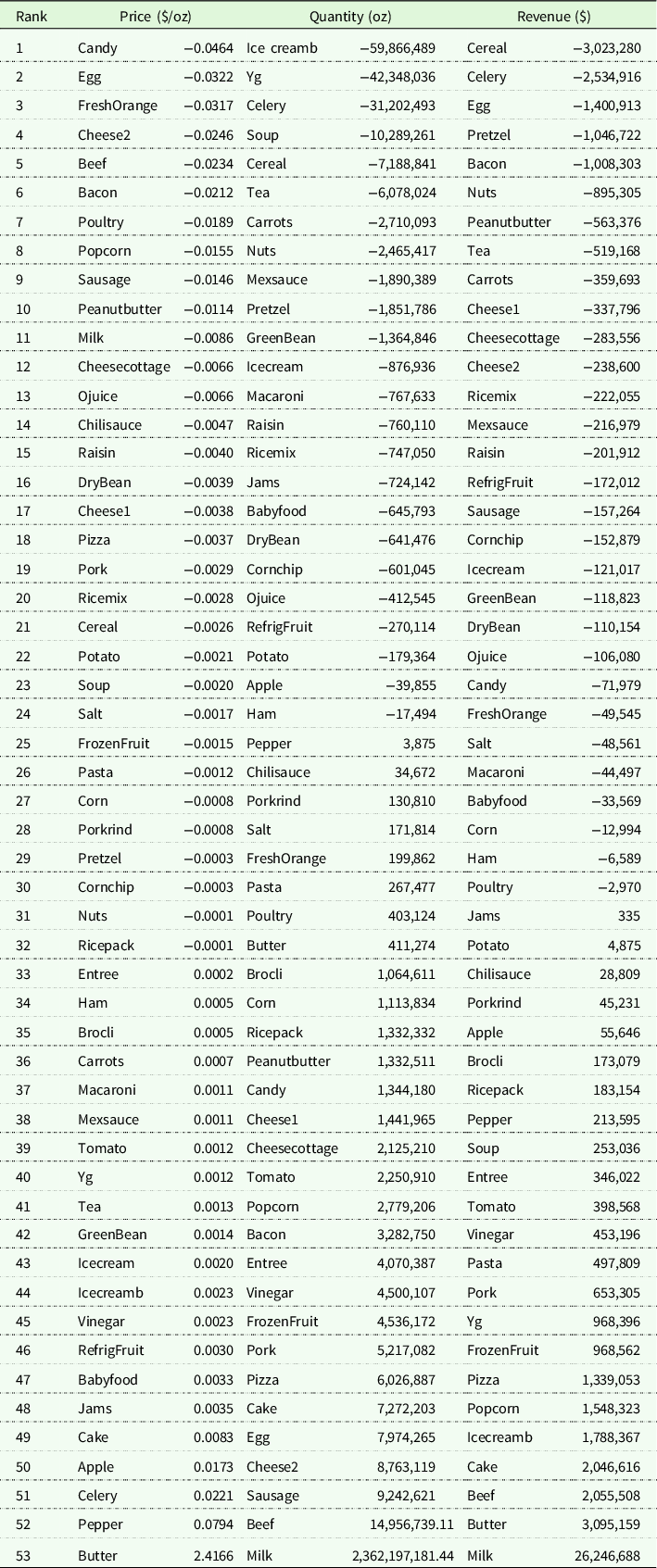
Table 4. Result of placebo test ranked by effect magnitude (adjusted)
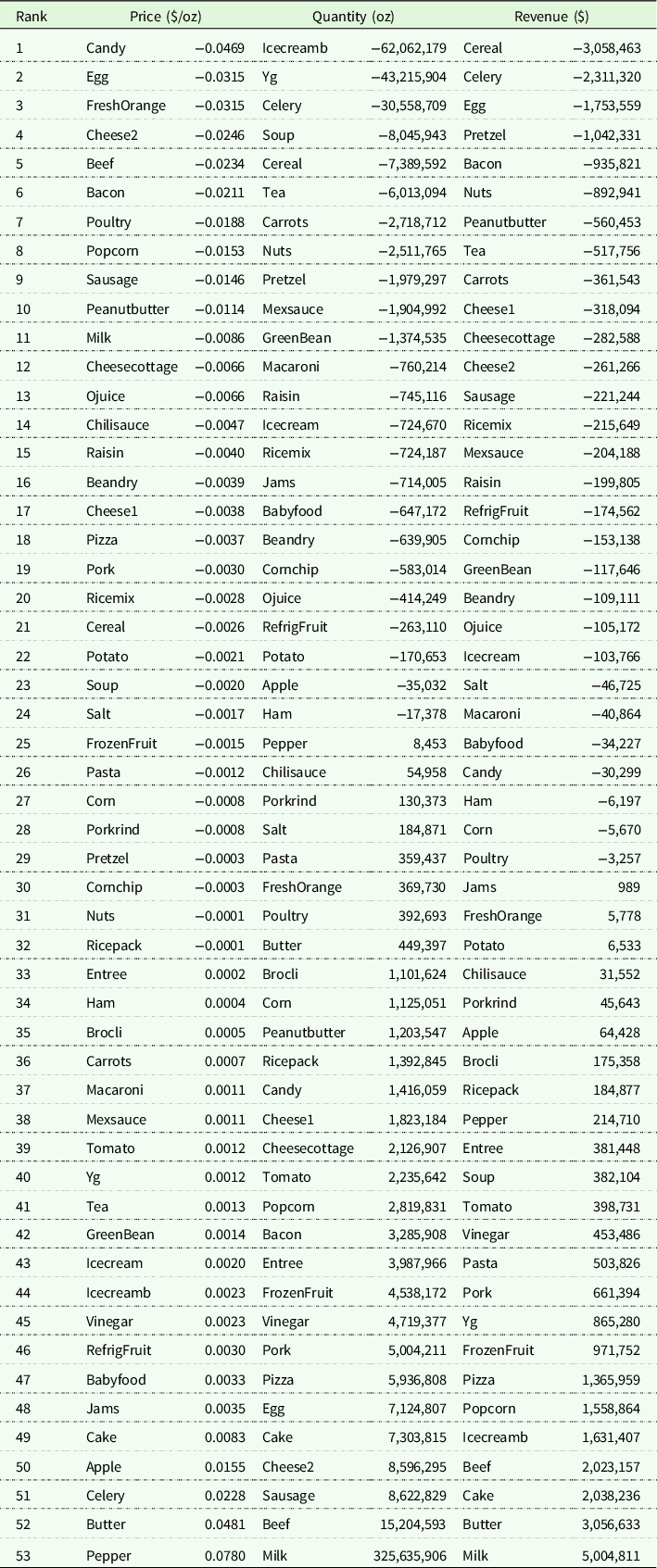
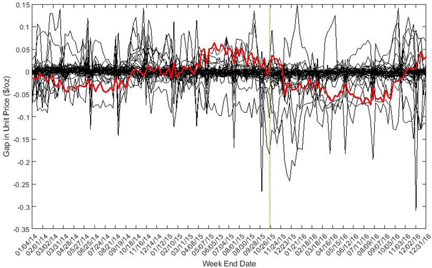
Figure 7. Placebo test – unit price gap of bacon.
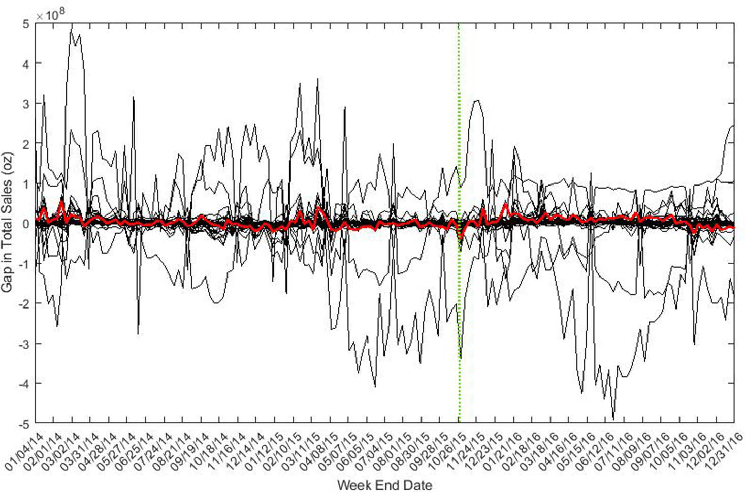
Figure 8. Placebo test – sales gap of bacon.
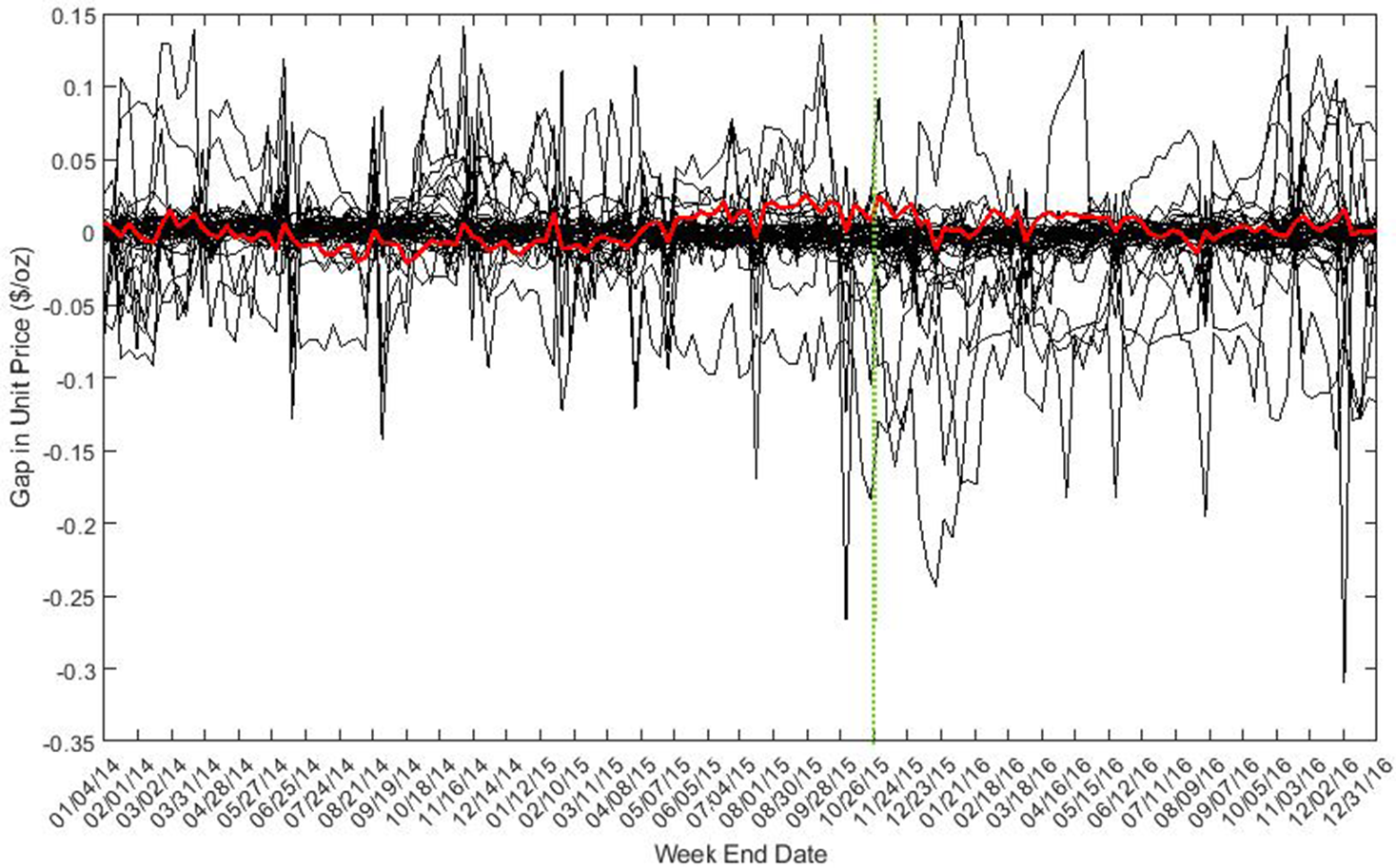
Figure 9. Placebo test – unit price gap of sausage.
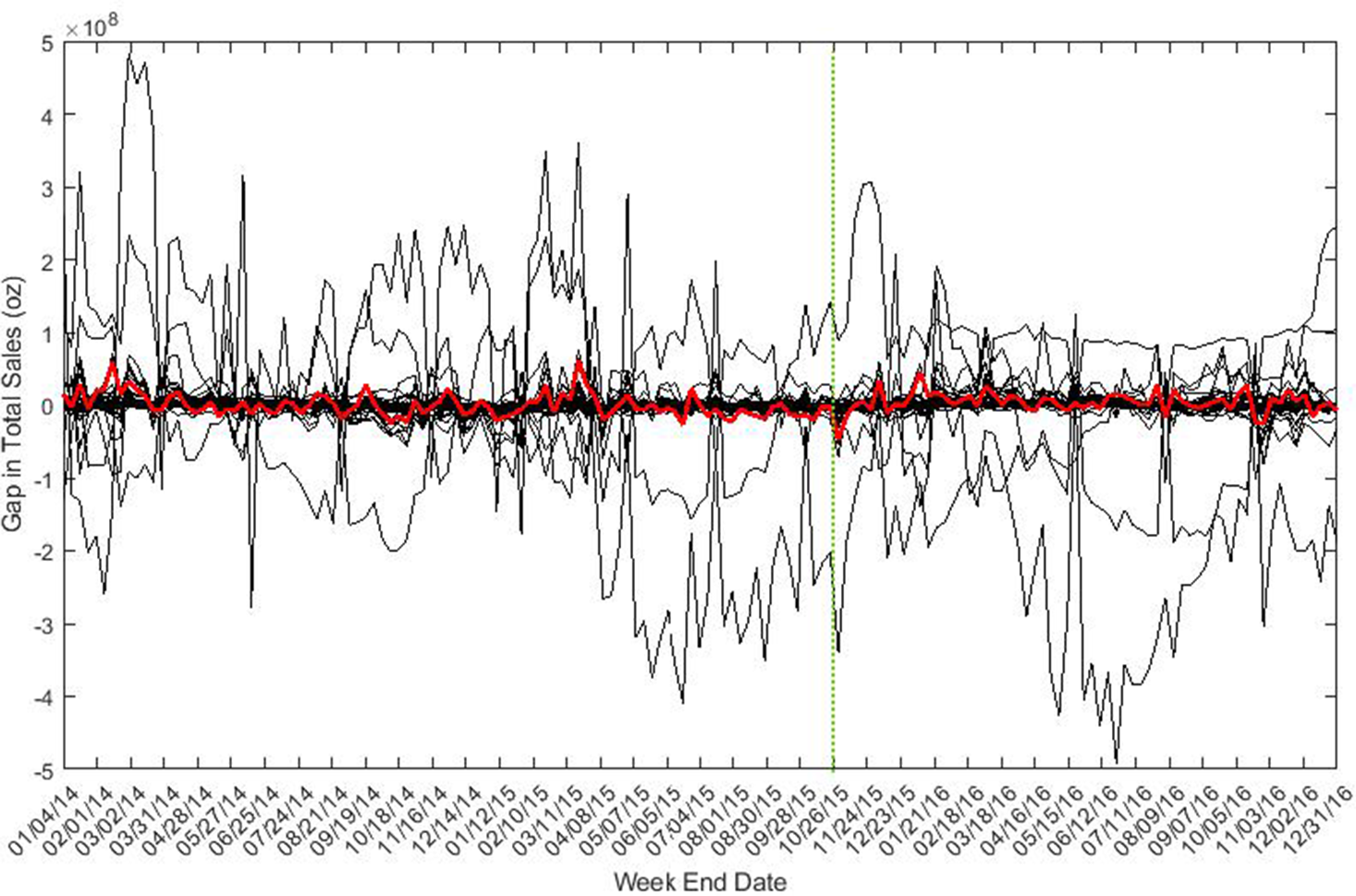
Figure 10. Placebo test – sales gap of sausage.
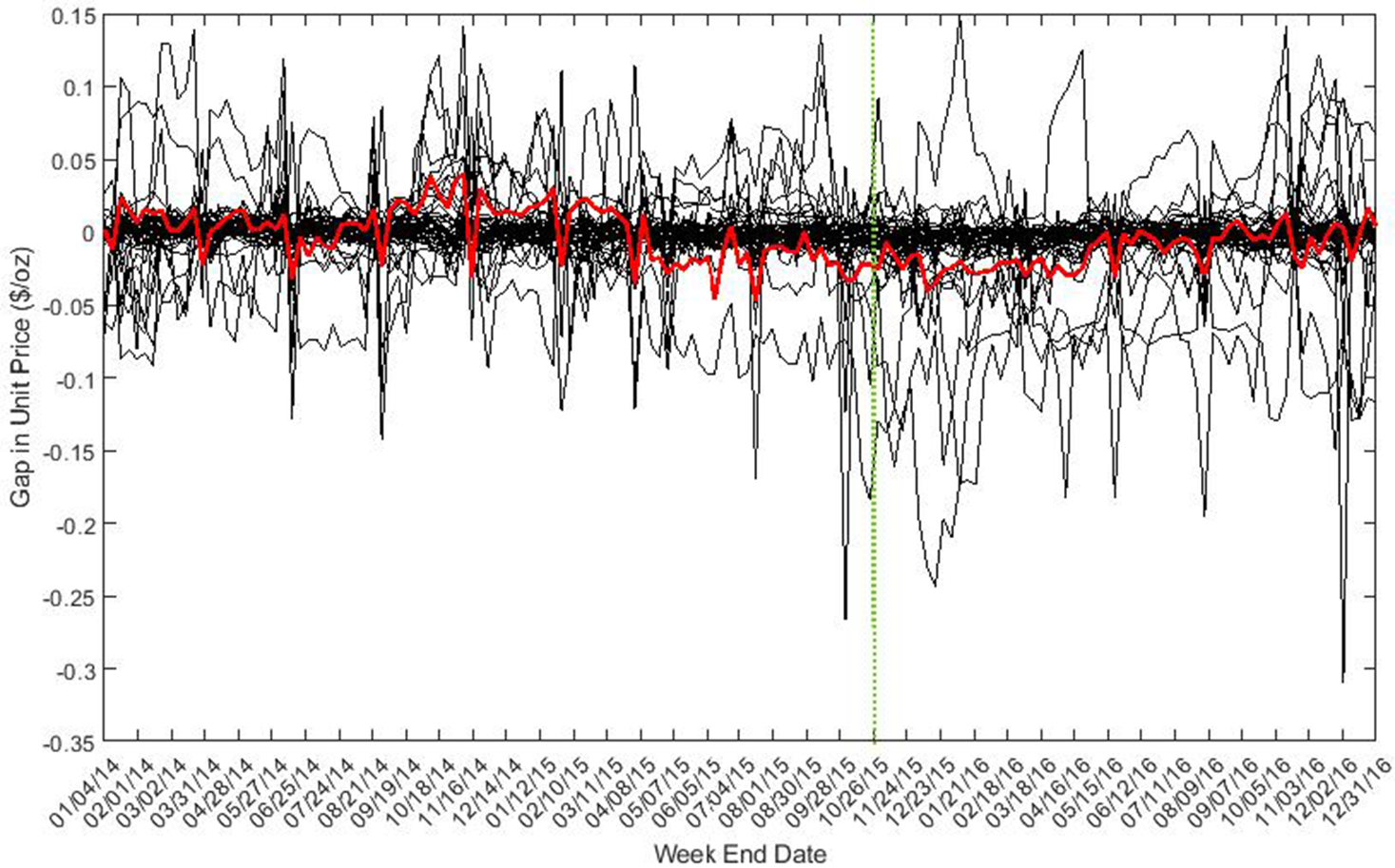
Figure 11. Placebo test – unit price gap of ham.
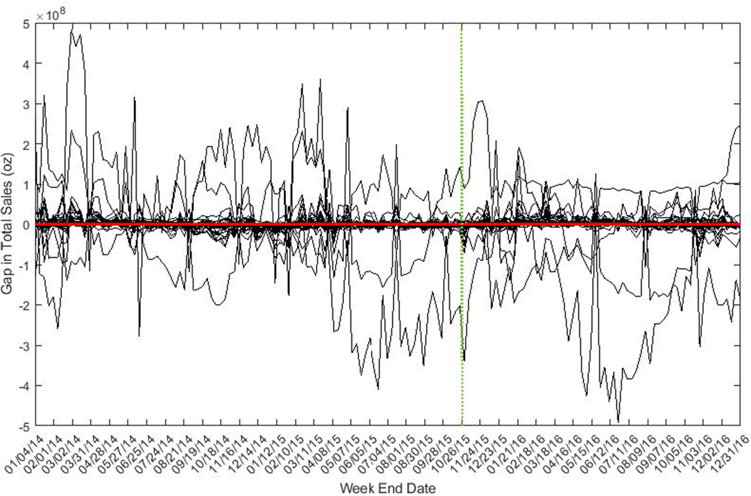
Figure 12. Placebo test – sales gap of ham.
From the results of placebo tests, we find only bacon price decreased significantly compared with changes in placebo products. We didn’t find statistically significant price reductions for ham and sausage. Changes in sales of bacon and ham were not statistically significant after the intervention as compared to changes in the placebo products; however, sausage quantity sold significantly increased.
In addition to the processed meat products, we further included fresh meat categories such as beef, poultry and pork in our analysis. We applied SCM on these categories by assuming fresh meat had also been affected by the IARC report. Among these fresh meat products, beef shows a statistically significant decrease in price after intervention. In addition, we find beef sales and revenue significantly increased after the intervention. However, we didn’t find statistically significant changes in price, sales, or revenue for pork and poultry products. All placebo test results for products in control group can be found in Table 5.
Table 5. Placebo test results for products in control group
Changes in demand
The preceding represented a reduced-form analysis to determine whether prices, quantities, or expenditures changed following the release of the IARC report. It remains an open question as to whether these changes are consistent with decreases in demand. Following results in Braekkan (Reference Braekkan2014) and Lusk and Tonsor (Reference Lusk and Tonsor2021), it is possible to determine the magnitudes of the demand shifts that occurred from the price and quantity changes, presuming one is willing to make assumptions about the magnitudes of the own-price elasticities of demand for the respective products.
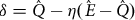
In particular, note that an approximation to changes in any underlying demand function can be expressed as: $\hat Q = \eta \hat P + \delta $
.
$\hat Q = \eta \hat P + \delta $
. $\hat Q$
is the proportionate change in quantity of the good demanded,
$\hat Q$
is the proportionate change in quantity of the good demanded, $\hat P$
is the proportionate change in price, and
$\hat P$
is the proportionate change in price, and $\eta $
is the own-price elasticity of demand.
$\eta $
is the own-price elasticity of demand.
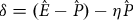
 $\delta $
is a demand shock representing the proportional change in consumers’ quantity demanded, and it is the magnitude of the horizontal shift in the demand curve expressed relative to the initial equilibrium quantity. This equation can be re-arranged to give the result:
$\delta $
is a demand shock representing the proportional change in consumers’ quantity demanded, and it is the magnitude of the horizontal shift in the demand curve expressed relative to the initial equilibrium quantity. This equation can be re-arranged to give the result: $\delta = \hat Q - \eta {\hat P^.}$
Thus, given an estimate of the percent change in quantity and price (provided in Table 1), and an assumption about the elasticity of demand,
$\delta = \hat Q - \eta {\hat P^.}$
Thus, given an estimate of the percent change in quantity and price (provided in Table 1), and an assumption about the elasticity of demand, $\eta $
, one can estimate the size and magnitude of a demand shift,
$\eta $
, one can estimate the size and magnitude of a demand shift, $\delta $
.
Footnote 3
$\delta $
.
Footnote 3
Tonsor and Lusk (Reference Tonsor and Lusk2021) recently estimated demand elasticities for disaggregate pork products in 51 retail markets across the USA using retail scanner data. The expenditure weighted average own-price elasticity across the 51 markets they studied was −0.87 for bacon, −3.38 for breakfast sausage, −2.53 for dinner sausage, and −1.47 for all pork products (they did not have a separate ham category). Given these demand elasticities, (−0.87 for bacon, −2.53 for sausage, and using the overall pork elasticity of −1.47 for ham), and the percent price and quantity changes in Table 1, the resulting calculations for $\delta $
are −2.13%, −8.4%, and −6.59% for bacon, sauage, and ham, respectively. In all three cases, the pattern of price and quantity changes we estimate are consistent with an inward and downward shift in demand following the release of the IARC report.
$\delta $
are −2.13%, −8.4%, and −6.59% for bacon, sauage, and ham, respectively. In all three cases, the pattern of price and quantity changes we estimate are consistent with an inward and downward shift in demand following the release of the IARC report.
Of course, these results depend on the magnitudes of the assumed own-price demand elasticities. We are not aware of other recent estimates of retail demand elasticities for disaggregate pork products in the USA, but Hailu, Vyn, and Ma (Reference Hailu, Vyn and Ma2014) found, using Canadian scanner data, own-price elasticity estimates of −1.126, −2.264, and −0.781 for bacon, sausage, and ham. Akaichi and Revoredo-Giha (Reference Akaichi and Revoredo-Giha2016), using Scottish scanner data, estimated own-price elasticities of −1.306, −1.210, and −1.292 for bacon, sausage, and ham. The elasticity estimates from these two additional sources, when coupled with the estimated price and quantity changes from this paper, also imply an inward shift in demand for all three products caused by the IARC report. In general, the most inelastic demand could be while continuing to imply an inward demand shift is −0.55 for bacon and −1.12 for sausage. For ham, no reasonable demand elasticity would imply anything other than an inward demand shift. Footnote 4
Changes in supply
Analogous to the demand changes calculated in the preceding sub-section, it is possible to determine the magnitudes of the supply shifts that occurred from the price and quantity changes if one is willing to make assumptions about the magnitudes of the own-price elasticities of supply (see Braekkan (Reference Braekkan2014) and Lusk and Tonsor [Reference Lusk and Tonsor2021]). In particular, note that an approximation to changes in any underlying supply function can be expressed as: $\hat Q = \varepsilon \hat P + \lambda $
.
$\hat Q = \varepsilon \hat P + \lambda $
. $\varepsilon $
is the own-price elasticity of supply,
$\varepsilon $
is the own-price elasticity of supply, $\lambda $
is the horizontal supply shift expressed as a proportion of the initial equilibrium quantity, and
$\lambda $
is the horizontal supply shift expressed as a proportion of the initial equilibrium quantity, and $\hat Q$
and
$\hat Q$
and $\hat P$
are as previously defined. Re-arranging this equation implies:
$\hat P$
are as previously defined. Re-arranging this equation implies: $\lambda = \hat Q - \varepsilon {\hat P}.$
Thus, given an estimate of the percent change in quantity and price (provided in Table 1), and an assumption about the elasticity of supply,
$\lambda = \hat Q - \varepsilon {\hat P}.$
Thus, given an estimate of the percent change in quantity and price (provided in Table 1), and an assumption about the elasticity of supply, $\varepsilon $
, one can estimate the size and magnitude of a supply shift,
$\varepsilon $
, one can estimate the size and magnitude of a supply shift, $\lambda $
.
$\lambda $
.
We are not aware of any product-specific retail pork supply elasticities, but there are several estimates of the farm-level supply elasticities of hogs in the literature, most suggesting highly inelastic supply, particularly in the short run. Taking a simple average of the short-run hog supply elasticities in Boetel, Hoffmann, and Liu (Reference Boetel, Hoffmann and Liu2007) and Holt and Moschini (Reference Holt and Moschini1992) and the supply elasticities in Lemieux and Wohlgenant (Reference Lemieux and Wohlgenant1989) and Suh and Moss (Reference Suh and Moss2017) suggests a supply elasticity of about 0.19. Given this elasticity, and the estimated price and quantity changes in Table 1, we calculate horizontal supply shifts of 4.8% for bacon, 7.9% for sausage, and −6.4% for ham. If the retail-level supply elasticity is more elastic than the farm-level supply elasticity, as suggested by results in Kinnucan and Zhang (Reference Kinnucan and Zhang2015), at a value of, say, 1, the implied demand shifts are of the same signs. At a supply value of 1, we calculate horizontal supply shifts of 10.1% for bacon, 12.7% for sausage, and −6.3% for ham.
The results in this section and the preceding one provide some insights into the observed price and quantity changes. For bacon and sausage, demand shifted inward at the same time supply shifted outward. For both products, this resulted in higher quantities but lower prices. For sausage, both demand and supply shifted inward following the release of the IARC report, resulting in lower prices and lower quantities.
Conclusions
In this study, we investigated how the widely discussed IARC report, indicating processed meat products were a type 1 carcinogen, affected market outcomes for processed meat. The information released from the report serves as an intervention which could potentially affect consumers’ perception of the healthiness of processed meat products. To explore this intervention effect, we compare the changes of price and sales for three major processed meat products, bacon, sausage, and ham, before and after the IARC report release date. We constructed a synthetic control group to simulate the counterfactual outcomes that would have occurred had the report not been released. By comparing observed outcomes with the constructed synthetic outcomes, we obtain insights on whether consumer demand changed in response to the report.
Our results show bacon price fell by 6.54% and bacon sales increased by 3.56% in the year following the IARC report release date. The price reduction is statistically significant compared with placebo products, which were not likely affected by the report information, while the quantity change was not larger than that likely to have been caused by chance. If we couple the estimated price and quantity changes with an estimate of the own-price elasticitiy of demand, we find that the demand curve for bacon shifted inward by about 2% and the supply curve shifted out by about 4.8%. We did not find significant changes in price, sales, or expenditures of ham or sausage, but the pattern of price and quantity changes is consistent with inward demand shifts of about 8% for sausage and 6.6% for ham. The price and quantity changes also suggest an outward shift in supply for sausage and an inward shift in supply for ham following the IARC report release.
In addition, we found fresh beef sales and revenue increased and fresh beef prices fell significantly after the report. The IARC report also noted the impacts of red meat consumption and health outcomes, classifying red meat as a type 2 carcinogen, and the findings here suggest that even this lesser association (type 2 vs. type 1 carcinogen) had market impacts. In addition to beef, we also explored changes in the prices, sales, and revenues for fresh chicken and pork, which might also serve as substitutes for processed meat. However, unlike beef, we did not observe significant changes for these products.
This study only investigated selected processed meat products, bacon, sausage, and ham. Future research might identify whether and to what extent other processed meats, such as hot dogs, canned meat, or lunch meat, might have been more or less impacted by the release of the report. This paper highlights the utility of the SCM in estimating such causal impacts.
Funding statement
This research received no specific grant from any funding agency, commercial or not-for-profit sectors.
Conflicts of interest
Lusk has conducted consulting work or given paid presentations for organizations such as: Beef Cattle Research Fund, Corn Refiners Association, National Pork Board, National Pork Producers Council, North American Meat Institute, Food Marketing Institute, and Cattlemen’s Beef Promotion and Research Board. None of these organizations supported or had any input on this research paper.
Data availability statement
Researcher(s) own analyses calculated (or derived) based in part on data from Nielsen Consumer LLC and marketing databases provided through the NielsenIQ Datasets at the Kilts Center for Marketing Data Center at The University of Chicago Booth School of Business. The conclusions drawn from the NielsenIQ data are those of the researcher(s) and do not reflect the views of NielsenIQ. NielsenIQ is not responsible for, had no role in, and was not involved in analyzing and preparing the results reported herein.


 Open access