


1. Introduction
Snow can be studied using images from serial sections or from grains taken from a snow sample. The first approach (Reference Good, Hunt and GuyenneGood, 1989) preserves the snow structure and allows observation of the grain connections. The second approach, used in this study; focuses on the grain characteristics.
We developed and validated a system allowing the description of snow-grain morphology. It can be used to improve the parameterization of the mctamorphism function in snow models (e.g. Crocus, Reference Brun, Martin, Simon, Gendre and Coléou.Brun and others, 1989,Reference Brun, David, Sudul and Brunot1992). The objective measures obtained by using this system may also be useful for calibrating snow-cover data acquired by remote-sensing techniques.
The first studies at the Centre d'Études de la Neige were conducted in 1985. Snow grains were observed through a binocular lens. The images were captured using an analog video camera (SONY DXC101 mono CCD, definition 320 lines, sensitivity 30 lux, ratio signal/noise 48 dB) and stored in analog form on video tape (SONY U-MATIC SP V09006, definition 280 lines, ratio signal/noise 46 dB). Subsequently, these images were converted from video sequences to a digital pixel image with a frame grabber (MID). The final resolution was 256 × 256 pixels with 64 grey levels.
This system was used in a quantitative study of dry-snow metamorphism in the presence of various temperature gradients (personal communication from G. Brunot, 1986) but had some hardware and software disadvantages (image distortion, low speed, etc.). The rapid improvement in computers, video techniques and image-analysis software allows new possibilities today. A recent upgrade of the image-processing system made it possible to develop a semi-automated analysis software of snow-grain images. A systematic exploration of all snow types began and led to an automatic determination of snow types from the morphology of the grains.
2. Acquisition and Image Analysis
2.1. Acquisition
The snow samples are either taken in the field or produced by a snow-metamorphism experiment in a cold room. In the former ease, the sample is transported in iso-octane (Reference Brun and Pahaut.Brun and Pahaut, 1991).
The snow grains are arranged on a glass plate and isolated as well as possible. A light source is placed below the plate and a camera (SONY DXC 755P, 3CCD, definition 750 lines, sensitivity 13 lux, ratio signal/noise 58 dB) takes 2D monochrome pictures of the grains through a binocular lens (LEICA M240). The images are stored on a video disk (SONY laser videodisc recorder LVR-4000P, definition 700 lines). A snow sample consists of a reference image (circular disk with known radius) followed by around 15 images of grains (not less than 30 grains are needed to obtain stable results) as shown in Figure 1. According to the snow type, the magnification varies from 8 to 12.5 and the number of grains in an image from 1 10 10. With a magnification equal to 12.5, the size of an image is around 5 × 4 mm.

Fig. 1. Grain images from a sample taken during a low gradient metamorphism experiment and used for test (time 87 hours in Figure 11). The diameter of the circular disk used for calibration is 3 mm. The magnification is × 12.5.
2.2. Image Enhancement
The images are digitized into a personal computer with a frame grabber (Matrox Meteor) and commercial software (Visilog from NOESIS). The resolution of the resulting image is 360 × 270 pixels with 256 grey levels. Then, the following treatments arc applied:
Transformation of the grey level images to binary images.
Filling of the particles.
Elimination of the particles whose sizes are lower than three pixels by applying an opening.
Elimination of grains truncated on the edge of the image.
Elimination of particles with a surface lower than a threshold chosen by the operator, in order to eliminate the chip of grains.
Numbering of the particles.
Extraction and sorting of the contours.
Figure 1 shows a typical snow sample. A magnification of 12.5 is used and a pixel is a square whose sides are 0.0145 mm long.
2.3. Image Analysis
For each grain, the following five parameters are calculated: the surface S, the maximum length L, the perimeter P, the parameter ![]() (which characterizes the dendricity of the grains (1 for a circle), the parameter
(which characterizes the dendricity of the grains (1 for a circle), the parameter  (which characterizes the elongation (1 for a circle).
These five parameters are strongly dependent on the arrangement of the grains: the grains should be separated. Thereafter, the maxima, minima, mean and standard deviation of these parameters of the snow sample are also calculated. Then the parameter ![]() is introduced. It is more reliable than
is introduced. It is more reliable than ![]() because it limits the impact of small grains in the sample.
because it limits the impact of small grains in the sample.
From all the contours of the sample, the calculated parameters are:
The curvature for each pixel (method discussed in section 3).
The mean and standard deviation of concave and convex curvature of the sample.
The mean concave and convex radius, being defined as the inverses of the mean curvatures.
The maxima and minima of the concave and convex curvature.
The distribution histogram of the radii (radii larger than 2 mm are grouped in a singled class).
3. Radius Calculation and Validation
The mean convex radius of curvature is the most important parameter used to characterize a snow sample. Since calculation of the radius was not available in the software Visilog it was developed locally and introduced into the software.
Only the mean convex radius is used, because the mean concave radius is too dependeut on the grain arrangement (particularly if polycrystalline grains are present).
3.1. Tangents Method
The radius of curvature is calculated in each pixel of the grain periphery, using an even number N pixels on each side of the considered pixel; N is chosen by the operator.
The tangent in each pixel p is calculated first. It is the straight line defined by the pixels P 1 and P 2 of the periphery (Fig. 2).

Fig. 2. Method by determination of tangents. Calculation of the radius of curvature in P using 21 pixels (N = 10). A square is a pixel of the grain peripher).
The radius of curvature is the radius of the circle tangent to the tangents in P 1 and P 2 (D is the distance between P 1 and P 2). In some cases (pixels on a straight line), a fixed large value (by default 200 pixels) is assigned.
3.2. Use of a Smoothing Function
In this method, the grain periphery is locally (N pixels on each side of the pixel considered) fitted with a second-order polynomial function.
First, the system looks for the coordinate axes in which a maximum of increasing x coordinates is found on both sides of the point P. The axis system is rotated clockwise with a ![]() angle several times (Fig. 3). For each transformation, the number of increasing x coordinates is calculated. The search is stopped when this number reaches
angle several times (Fig. 3). For each transformation, the number of increasing x coordinates is calculated. The search is stopped when this number reaches ![]() . If it is lower than
. If it is lower than ![]() in the eight axis systems, we retain the axis system in which this number is maximum. But, if it is lower than a minimum value fixed by the operator (the default value is 5), the radius calculation is not done.
in the eight axis systems, we retain the axis system in which this number is maximum. But, if it is lower than a minimum value fixed by the operator (the default value is 5), the radius calculation is not done.

Fig. 3. Smoothing-function method. Research of the best rotation and theJunction f(x).
In a second step, a second-order regression is done using the points selected above.
The smoothing function ![]() is determined and the radius R is given by:
is determined and the radius R is given by:

In some cases, this function is undetermined and the calculation of the radius cannot be done.
The radii are calculated along the contours of the particles. When the calculation cannot be done on a pixel, the value calculated on the previous pixel is assigned to it.
The curvatures (inverses of the radii) are stored in a file. At the end of processing the sample, the means and standard deviations are calculated using this file.
3.3. Validation and Choice of the Method
In order to validate the radius calculation and determine the best method and number of pixels ![]() , a systematic-analysis of circular disks with various sizes has been undertaken. The radii of the disks were: 0.125, 0.25, 0.5, 0.75 and 1.5 mm (respectively around 9, 17, 34, 52 and 103 pixels). Two series of analyses were performed: one with isolated disks, and the second with aggregated disks. A magnification of 12.5 was used and the two methods were tested. The parameter
, a systematic-analysis of circular disks with various sizes has been undertaken. The radii of the disks were: 0.125, 0.25, 0.5, 0.75 and 1.5 mm (respectively around 9, 17, 34, 52 and 103 pixels). Two series of analyses were performed: one with isolated disks, and the second with aggregated disks. A magnification of 12.5 was used and the two methods were tested. The parameter ![]() was successively set to 13, 17, 21 and 25.
was successively set to 13, 17, 21 and 25.
Figure 4 shows the results for the mean convex radius (MGR.). For values of ![]() lower than 17 and for disks whose radii are larger than 0.5 mm, the radii are underestimated by both methods.
lower than 17 and for disks whose radii are larger than 0.5 mm, the radii are underestimated by both methods.

Fig. 4. Relative error of the mean convex radius: percentage of error on isolated and aggregated circular disks in the function of the parameter ![]() .
.
In the case of aggregated disks, the tangent method with ![]() larger than 13 gives poor results on small disks. The smoothing method leads to errors around 10% from 17 to 25 pixels.
larger than 13 gives poor results on small disks. The smoothing method leads to errors around 10% from 17 to 25 pixels.
In all cases, the smoothing method is more stable and gives a smaller relative error than the tangent method. It is therefore the preferred method.
As the diameter of most snow grains is smaller than 2 mm, the use of 17 pixels seems to be the best compromise. In most cases, the errors in the radius calculation are lower than 10%. For larger snow grains, one can return to a favourable situation by reducing the magnification during the image recording.
In this study, the smoothing method using ![]() equal to 17 pixels was used for radius calculations in all snow-samples. The magnification was usually 12.5 and was reduced for samples with larger grains.
equal to 17 pixels was used for radius calculations in all snow-samples. The magnification was usually 12.5 and was reduced for samples with larger grains.
Recording of images of a sample in the cold laboratory (around 15 images) requires about 10–15 minutes. The image acquisition and the complete processing (included the automatic determination) takes about 10 minutes. For the two computing methods, the times required are almost the same.
4. Automatic Determination of Snow Types
4.1. Learning
In order to obtain a full range of parameters calculated on all snow types, 65 snow samples were investigated. They were distributed as follow:
Twelve precipitation particle samples (1 in the International Classification: +), three samples with precipitation and recognizable particle characteristics (1,2: +, /), six recognizable or decomposing particle samples (2: /), ten samples with recognizable particles and rounded-grain characteristics (2, 3: /, ·), five rounded-grain samples (3: ·), seven wet-grain samples ![]() , nine faceted-crystal samples (4: □), ten depth-hoar samples (5: ^) and three samples with depth-hoar and wet-grain characteristics
, nine faceted-crystal samples (4: □), ten depth-hoar samples (5: ^) and three samples with depth-hoar and wet-grain characteristics ![]() .
.
The samples were classified visually by several experts in accordance with the International Classification (Reference ColbeckColbeck and others, 1990).
4.2. Selection of Informative Parameters
Some parameters are too dependent on the arrangement of the grains (contacts between grains) and were rejected: surface, perimeter and length. Several graphics showing the results for two parameters were plotted. An example is shown in Figure 5 for the mean convex radius and the standard deviation of convex curvature (SDC). In order to clarify the visualization, only 49 samples pertaining to a single snow type are plotted. The points corresponding to a given snow type are usually grouped and more or less separated from the others. This is not true for the precipitation particles (+) whose points can be found together with the recognizable particles (/), rounded grains (·) and faceted crystals (□). This situation was observed for most parameters because of the high variability of the shape of precipitation particles in Nature. Because of these difficulties, it was decided to focus only on the other snow types.

Fig. 5. Distribution in the learning file for the parameters MCR and SDC.
The following parameters were selected:
Mean convex radius (MCR). This parameter gives information on the grain-size. Moreover, it is very little dependent on the choice of different images from the same snow sample.
Standard deviation of convex curvature (SDC). This parameter, depending on the regularity of the grains peripheries, also has the same behaviour as the previous one.
Ratio standard deviation of convex curvature/mean convex curvature (SDC/C). This ratio allows better discrimination between snow samples with the same mean curvature or the same standard deviation. In Figure 6, rounded grains and faceted crystals are somewhat better separated than in Figure 5.
![]() . This parameter increases with dendricity and decreases for granular snow. Unlike the parameters above, it depends on the arrangement of the grains.
. This parameter increases with dendricity and decreases for granular snow. Unlike the parameters above, it depends on the arrangement of the grains.
Histo. The analysis of detailed results for the calculation of MCR showed that the histogram is linked to the snow type. Figure 7 compares the radii histograms for two snow types (rounded grains and faceted crystals) having a very close mean convex radius. An empirical parameter (called histo) has been built to take into account the histogram differences.

Fig. 6. Distribution in the learning file for the parameters MCR and SDC/C.

Fig. 7. Histograms of the mean convex radius. Comparison between rounded grains und faceted to crystals. The histogram corresponds to all the pixels of the contours of the grains. The number of pixels of the contours of a sample is around 10 000.
It is defined by ![]() is the maximum ordinate for convex radii smaller than 2 mm,
is the maximum ordinate for convex radii smaller than 2 mm, ![]() is the abscissa corresponding to
is the abscissa corresponding to ![]() and np is the ordinate corresponding to convex radii larger than 2 mm.
and np is the ordinate corresponding to convex radii larger than 2 mm.
4.3. Method for Determining Snow Types
A determination based on simple thresholds was unsuccessful, because the parameters show considerable overlap. Figure 8 also shows that the calibration data are sparse.
Another approach was attempted. Using these data, a frequency distribution was established between each snow type and each parameter. This distribution expresses the likelihood of the relationship between this snow type and each class of values of this parameter. It takes values (weightings) between 0 and 1. The 0 value means that the sample cannot relate to this type. On the contrary, 1 means that the sample, with respect to this parameter, shows the characteristics of the type.

Fig. 8. Weightings corresponding to each snow type for the five parameters from the values taken in the calibration database.
Figure 8 shows the values for each parameter calculated from the calibration data and the estimated weightings for each class of values. The assignment of these weightings is partially based on the values calculated from the calibration data, and improved by expert knowledge. In addition, the weightings are adjusted by trial and error using the 53 samples of the calibration data (65 samples minus the 12 samples with precipitation particles).
The determination of the characteristics of a sample is obtained by multiplying each of the five weightings, corresponding to the five parameters, for each of the five snow types.
The sample feature is described by the five values obtained. Features of more than one snow type can be detected in a sample. A nearest-neighbour approach, using these five parameters, has also been tried. However this statistical approach was not fully successful because of the far too limited database.
4.4. Determination of Additional Parameters
In snow models, snow types are usually characterized by continuous variables, mainly grain-size. It seems possible to link the sample characteristics to model variables. Here we present a first attempt using the snow model Crocus. In this model, the snow morphology is characterized by two figures varying between 0 and 1: dendricity and sphericity for recent snow; size and sphericity for granular snow.
The dendricity varies between 1 for precipitation particles and 0 for granular snow.
The sphericity varies between 1 (for rounded grains and wet grains) and 0 (for faceted crystals and depth hoar). It is arbitrarily fixed at 0.5 for precipitation particles.
After examining the results (Fig. 8), the following correspondence between the snow characteristics and the Crocus formalism is proposed:
The parameter ![]() varies roughly from 2 (wet grains) to 12 (dendritic fresh snow). The estimated dendricity follows this evolution but it varies from 0 to 1.
varies roughly from 2 (wet grains) to 12 (dendritic fresh snow). The estimated dendricity follows this evolution but it varies from 0 to 1.
The estimated sphericity varies from 0 to 1 when the ratio SDC/C varies from 1.3 (depth hoar) to 0.8 (rounded grains and wet grains).
The estimated size is given by the mean convex radius. To take into account the angular form of faceted crystals and depth hoar, the diameter is multiplied by the above ratio. This is somehow arbitrary.
All the estimated characteristics are included in the outputs of the following analysis.
4.5. Tests
Figure 9 shows the results of the analysis from the sample shown in Figure 1. The calculated parameters are given together with the histogram of convex and concave radii. Below, the weightings for each snow type are given. Three snow types are excluded (wet grains, faceted crystals and depth hoar). The two others present very similar scores. This means that the sample has some characteristics of re-cognizable particles and some characteristics of rounded grains. Finally, values to be used in the snow model Crocus are also given.

Fig. 9. Analysis of the grains shown in Figure 1: histograms of the radii and output of the objective determination.
A treatment of 37 independent test samples has been undertaken. The results are summarized in Figure 10 using the following rules: when several snow types are found, the second is ignored if its proportion is less than 5% (a possible third snow type is always ignored)

Fig. 10. Contingency table for the final test. 1: visual determination. 2: automatic determination.
Twenty-three analyses (62%) gave goods results.
Thirteen others (35%) gave a result rather close to the visual observation.
For instance, four samples were recognized as ![]() (wet grains/faceted crystals) but were classified as
(wet grains/faceted crystals) but were classified as ![]() (wet grains/depth hoar) by the experts.
(wet grains/depth hoar) by the experts.
One snow sample consisting of recognizable particles with a significant proportion of needles was identified as “faceted crystals”. Moreover, a beginning of angular shape was observed because of the large temperature gradient during two nights. The system found only faceted-crystal characteristics because of the straight periphery of the needles. This problem is similar to that encountered with precipitation particles.
4.6. Metamorphism Experiments
Two samples consisting of recognizable decomposing precipitation particles were submitted to a metamorphism experiment in a cold laboratory. The first sample was kept at –5°c (without temperature gradient) and the second was submitted to a large temperature gradient (1°C cm1 at a mean temperature of ×1°C). The evolution of the snow type was followed by regular sampling. Figure 11 shows the evolution of the mean convex radius and the standard deviation of convex curvature. The slow increase in the mean convex radius and the absence of a temperature gradient, also shown by Reference Brown, Edens and Sato.Brown and others (1994), was correctly detected (+0.04 mm after 1000 hours). In this metamorphism experiment, the smoothing of the periphery of the grains is associated with a regular decrease in the standard deviation of convex curvature. In the large-gradient experiment, the grain growth is rapid as expected. In both cases, the snow-type evolution was correctly detected by the semi-automated analysis (Fig. 12).
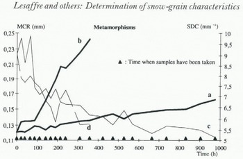
Fig. 11. Evolution of the mean convex radius (MCR) and the standard deviation of convex curvature (SDC) during two snow-metamorphism experiments. Isothermal metamorphism: (a) MCR; (c)SDC; Large-gradient metamorphism: (b)MCR: (d) SDC.

Fig. 12. Semi-automatic determination of snow types during the metamorphism experiments.
5. Conclusion
Fresh snow is characterized by a great variety of shapes. Therefore, it is not possible to distinguish them by using the five parameters described in this study. During the metamorphism process, the different states can be more easily determined and the results of the semi-automatic determination of snow types are largely positive (e.g. 62% looking only at the main types and another 35% if intermediate snow types are also rated as successful).
For fresh snow, only dendricity and sphericity are given.
The mean convex radius given by the system is very precise and stable as shown in the metamorphism experiments. The standard deviation of curvature and the distribution of the convex radii also play an important role in the objective determination process.
The parameter ![]() is linked to dendricity but it is very sensitive to the grain arrangement in the images. It is necessary to improve the separation of the grains to avoid biases in the analysis.
is linked to dendricity but it is very sensitive to the grain arrangement in the images. It is necessary to improve the separation of the grains to avoid biases in the analysis.
A larger learning file would have allowed a more precise determination of the weightings used in the system.
Nevertheless, the different snow types are well characterized by the five parameters selected. The objective determination proposed here allows comparison of snow samples represented by a sufficient number of singular grains on criteria independent of human observers.
Acknowledgements
We are grateful to A. Duclos (Transmontagne) and many colleagues of the Centre d'Études de la Neige who provided us with some of the snow images analysed in this study.
This research was supported by the EC Environment and Climate Research Program (contract ENV4-CT95-0076, Climatology and Natural Hazards).


