


1. Introduction
In three-dimensional (3-D) homogeneous isotropic turbulence (HIT), the injected energy transfers at a constant rate by nonlinear interactions to small scales until dissipation occurs. In the inertial range, where the scales are away from the energy-containing scale and the dissipation scale, from the Kármán–Howarth–Monin (KHM) equation (von Kármán & Howarth Reference von Kármán and Howarth1938; Monin & Yaglom Reference Monin and Yaglom1975), Kolmogorov (Reference Kolmogorov1941) obtained an asymptotic result for the longitudinal velocity structure function
 \begin{equation} \langle \delta u_L^3 \rangle =-\tfrac{4}{5}\epsilon r, \end{equation}
where  $\langle {\cdot } \rangle$ denotes the ensemble average, $\delta u_L = (\boldsymbol {u}' - \boldsymbol {u}) \boldsymbol{\cdot } \boldsymbol {r}_0$ is the longitudinal velocity difference with $\boldsymbol {u}' = \boldsymbol {u}(\boldsymbol {x} + \boldsymbol {r})$ , $\boldsymbol {r}$ the separation vector of two points with $\boldsymbol {r}_0=\boldsymbol {r}/|\boldsymbol {r}|$ a unit vector and $\epsilon$ is the energy dissipation rate. The corresponding energy spectrum $E(k) \sim k^{-5/3}$ is also widely observed (Obukhov Reference Obukhov1941; Frisch Reference Frisch1995), here $k$ is the wavenumber.
For the dynamics of scales larger than the forcing scale (large scales hereafter), since energy cascades from the forcing scale down to small dissipation scales, leaving no averaged upscale energy to the large scales, it has been conjectured that the large-scale dynamics of forced 3-D HIT can be described by the absolute equilibrium (Hopf Reference Hopf1952; Lee Reference Lee1952; Kraichnan Reference Kraichnan1973; Rose & Sulem Reference Rose and Sulem1978; Frisch Reference Frisch1995; Lesieur Reference Lesieur1997). The spectra of this equilibrium state follow the statistical mechanics of the truncated Euler equations, where energy equally distributes among all Fourier modes and the velocity distribution is Gaussian (Rose & Sulem Reference Rose and Sulem1978). Based on Liouville's theorem (Lee Reference Lee1952) and the Gaussian equipartition ensemble (Orszag Reference Orszag1977), Kraichnan (Reference Kraichnan1973) predicted the energy and helicity spectra
 \begin{equation} E(k) = \frac{4 {\rm \pi}\alpha k^2}{\alpha^2 - \beta^2k^2} \quad \mathrm{and} \quad \ H(k) = \frac{4 {\rm \pi}\beta k^4}{\alpha^2 - \beta^2 k^2}, \end{equation}
respectively. The coefficients  $\alpha$ and $\beta$ are determined by the energy and the helicity of flow. For non-helical flow, $\beta = 0$, leading to an energy spectrum $E(k) \sim k^2$. Numerical and experimental results have justified the large-scale statistical equilibrium in 3-D HIT (Cichowlas et al. Reference Cichowlas, Bonaïti, Debbasch and Brachet2005; Dallas, Fauve & Alexakis Reference Dallas, Fauve and Alexakis2015; Cameron, Alexakis & Brachet Reference Cameron, Alexakis and Brachet2017; Alexakis & Biferale Reference Alexakis and Biferale2018; Alexakis & Brachet Reference Alexakis and Brachet2019, Reference Alexakis and Brachet2020; Gorce & Falcon Reference Gorce and Falcon2022; Hosking & Schekochihin Reference Hosking and Schekochihin2023). The dynamics of scales larger than the forcing scale are of interest for many flows where the energy flux is zero, e.g. geophysical and astrophysical flow, and turbulent mixing in industrial processes (Dallas et al. Reference Dallas, Fauve and Alexakis2015). The large-scale statistical equilibrium is also reported in magnetohydrodynamic turbulent flows (Linkmann & Dallas Reference Linkmann and Dallas2016, Reference Linkmann and Dallas2017) and wave turbulence, such as capillary waves (Balkovsky et al. Reference Balkovsky, Falkovich, Lebedev and Shapiro1995; Michel, Pétrélis & Fauve Reference Michel, Pétrélis and Fauve2017), bending waves (Miquel, Naert & Aumaître Reference Miquel, Naert and Aumaître2021) and optical waves (Baudin et al. Reference Baudin, Fusaro, Krupa, Garnier, Rica, Millot and Picozzi2020).
However, the large-scale dynamics of the forced 3-D HIT differ from the absolute equilibrium of the truncated Euler equations. In the absolute equilibrium, the energy and helicity are conserved in an isolated system, where the initial conditions solely determine the statistical dynamics. Although the energy flux is zero on average for the large scales of forced 3-D HIT, Alexakis & Brachet (Reference Alexakis and Brachet2019) pointed out that the large-scale dynamics depend on the details of forcing. Due to the nonlinear interactions, there are transient energy transfers between the large and small scales. Here, the small scales include the forcing, inertial-range and dissipation scales. Therefore, the spectra quantitatively depart from those predicted by the absolute equilibrium.
In the free-decaying turbulence, ‘Saffman turbulence’ (Saffman Reference Saffman1967) predicts a similar spectrum, which, however, has different mechanisms from those of the forced turbulence (Batchelor & Proudman Reference Batchelor and Proudman1956; Davidson Reference Davidson2015). In the forced turbulence, averages over statistically steady states are considered and the large scales interact with small scales. In contrast, the flow is transient in the free-decaying turbulence and the forcing effect is absent.
An alternative way to distinguish different scales is to consider the separation space (Davidson & Pearson Reference Davidson and Pearson2005). This article focuses on the statistics of velocity structure functions at separations larger than the forcing scale. Gorce & Falcon (Reference Gorce and Falcon2022) studied the second- and third-order structure functions and found that they are independent of separation  $r$ of two measured points, which we believe is a result of low resolution. This article shows that the probability density functions (p.d.f.s) of velocity difference at large separations are close to, but deviate from, the Gaussian distribution. This deviation is measured by the p.d.f.s’ non-zero odd part, for which we propose a universal separate-variable form by normalizing the velocity difference using the combination of the downscale energy flux rate $\epsilon$ and the forcing wavenumber $k_f$. This is a conjugate of Kolmogorov's theory (Kolmogorov Reference Kolmogorov1941), where the invariant velocity difference p.d.f. in the inertial range is independent of the forcing scale and is obtained after normalizing the velocity by $(\epsilon r)^{1/3}$. Using the separate-variable-form p.d.f. and the exact expressions for the third-order structure functions, we calculate the analytical expressions for the odd-order structure functions, whose magnitudes’ slow decay in the limit of large separation implies a strong interaction between large- and small-scale structures.
2. Theory
We study the forced 3-D incompressible Navier–Stokes equations
 $$\begin{gather} \frac{\partial{\boldsymbol{u}}}{\partial{t}} + \boldsymbol{u} \boldsymbol{\cdot } \boldsymbol{\nabla} \boldsymbol{u} =- \boldsymbol{\nabla} p + \nu \nabla^2\boldsymbol{u} + \boldsymbol{F}, \end{gather}$$
 $$\begin{gather}\boldsymbol{\nabla}\boldsymbol{\cdot }\boldsymbol{u} = 0, \end{gather}$$
where  $p$ is the pressure, $\nu$ is the viscosity and $\boldsymbol {F}$ is the external forcing.
From the KHM equation (Frisch Reference Frisch1995), we have the relation between the longitudinal third-order structure function and energy injection rate in statistically steady 3-D homogeneous isotropic turbulence:
 \begin{equation} \frac{1}{r^2}\frac{\mathrm{d} }{\mathrm{d} r}\left( \frac{1}{r}\frac{\mathrm{d} }{\mathrm{d} r}\left({r^4 \langle \delta u_L^3 \rangle}\right) \right) =- 6{ \langle{\boldsymbol{F}\boldsymbol{\cdot }\boldsymbol{u}'+\boldsymbol{F}'\boldsymbol{\cdot }\boldsymbol{u}} \rangle}. \end{equation}
Here, the external forcing is delta-correlated in time. Since the divergent part of  $\boldsymbol {F}$ is absorbed by the fluid pressure, we assume $\boldsymbol {\nabla }\boldsymbol{\cdot }\boldsymbol {F} = 0$. So the power input term is known a priori, i.e. $\langle \boldsymbol {F}\boldsymbol{\cdot }\boldsymbol {u}'+\boldsymbol {F}'\boldsymbol{\cdot }\boldsymbol {u} \rangle = 2\langle \boldsymbol {F} \boldsymbol{\cdot }\boldsymbol {F}'\rangle$ (Bernard Reference Bernard1999; Srinivasan & Young Reference Srinivasan and Young2012; Xie & Bühler Reference Xie and Bühler2018). Since we focus on the dynamics for scales larger than the forcing scale, let us assume that the forcing effect is confined in the displacement space, i.e. there exists a finite scale $r_c<\infty$ such that the right-hand side of (2.2) equals $0$ when $r>r_c$, or the forcing effect decays fast enough, e.g. the right-hand side of (2.2) decays exponentially, then in the limit of large displacement, (2.2) gives
 \begin{equation} \langle{\delta u_L^3}\rangle \sim r^{-2}, \end{equation}
which is a universal scaling.
The neglect of forcing impact on the scales larger than the forcing scale is similar to the calculation of the third-order structure function in the energy inertial inverse-cascading range. In two-dimensional turbulence, due to the upscale energy flux, (2.2) contains an extra term, the large-scale damping (Xie & Bühler Reference Xie and Bühler2018) or energy temporal increasing (Lindborg Reference Lindborg1999), to dominate over the forcing effect. However, in our current 3-D turbulence scenario, the forward energy cascade prevents such a term. So, we seek a scenario where the forcing decays fast enough in the displacement space to avoid the impact of specific forcing forms and focus on the property of the Navier–Stokes equation. The choice of locality is stronger than the asymptotic locality, which has a power-function decay (Eyink Reference Eyink2005).
Thus, we introduce the type-I forcing, which decays exponentially, i.e.
 \begin{equation} \langle \boldsymbol{F}\boldsymbol{\cdot }\boldsymbol{F}' \rangle \sim \exp(-(rk_f)^2/4). \end{equation}
From dimensional analysis, the longitudinal third-order structure can be expressed as
 \begin{equation} \langle \delta u_L^3 \rangle = \frac{\epsilon}{k_f} g(k_fr). \end{equation}
Substituting (2.4) into (2.2), the type-I forcing leads to (Xie & Bühler Reference Xie and Bühler2019)
 \begin{equation} g_{I}(z) =-12\frac{\sqrt{\rm \pi} (z^2-6) \mathrm{erf}(z/2) + 6z\exp(-z^2/4)}{z^4}, \end{equation}
and in the large-scale limit,  $r \rightarrow \infty$, we obtain
 \begin{equation} \langle \delta u_L^3 \rangle_{I} \rightarrow -12 \sqrt{\rm \pi} \frac{\epsilon}{k_f^3 r^2}, \end{equation}
which is consistent with (2.3).
Considering that the strongly localized forcing in the displacement space is not always realized, e.g. the delta-forcing in the spectral space is usually used in numerical simulations, we discuss the structure functions in the spectral space. Noting that by using a Fourier transform, we can also express the right-hand side of (2.2) with the spectral energy injection rate  $\epsilon (k)$ as
 \begin{equation} - 12 \int_{0}^{\infty}\mathrm{d} k \,\frac{\varepsilon(k)}{kr} \sin(kr), \end{equation}
the confined forcing effect in the displacement space also implies a constraint of  $\varepsilon (k)$. Under the constraint of a finite total energy injection rate, an extreme case is associated with a delta concentrated energy injection rate, $\varepsilon (k)=\epsilon \delta (k-k_f)$. Here, $\varepsilon (k)$ is not an integrable function but is understood as a Dirac measure. So we introduce the type-II forcing with energy injected at a spherical shell, i.e. $|\boldsymbol {k}|=k_f$ with $\boldsymbol {k}$ the wavenumber vector. Now, solving (2.2), we obtain
 \begin{equation} g_{II}(z) =-12\frac{-z^2\sin(z) - 3z\cos(z)+3\sin(z)}{z^4}, \end{equation}
and it presents a  $r^{-2}$ envelope for $\langle {\delta u_L^3}\rangle$ in the limit of large displacement:
 \begin{equation} \langle \delta u_L^3 \rangle_{II} \rightarrow 12 \frac{\epsilon}{k_f^3 r^2} \sin(k_f r). \end{equation}
It should be noted that while the type-II forcing is local in spectral space, the corresponding forcing correlation follows  $\langle \boldsymbol {F}\boldsymbol{\cdot }\boldsymbol {F}' \rangle \sim \sin (K_fr)/r$, whose magnitude decays as a power function. So it is not strongly localized in the displacement space, but asymptotic local.
2.1. Expressions of p.d.f. and high-odd-order structure functions
In the first case, while the forcing decays exponentially with separation  $r$, the third-order structure function still decays slowly as $r^{-2}$, suggesting strong interactions between forcing and large scales. Since the large and forcing scales are well coupled, we hypothesize that the forcing mechanism dominates the dynamics of the no-flux regime (large scales). Therefore, the odd part of the probability distribution of velocity difference at large separations has a separate-variable form where the velocity difference is normalized by the combination of characteristic wavenumber $k_f$ and energy injection rate $\epsilon$:
 \begin{equation} \mathcal{P}_{odd}\left(\delta u_L, \epsilon, k_f, r\right) = \mathcal{P}_0\left(\delta u_L/\left({\epsilon}/{k_f}\right)^{1/3}\right) g(k_f r). \end{equation}
This expression is quite remarkable as a conjugate of Kolmogorov's theory, where the inertial-range p.d.f. of velocity difference is normalized using displacement as a characteristic spatial scale following  $\delta u_L/(\epsilon r)^{1/3}$.
Thus, in the no-flux range, the odd-order structure functions are obtained from a direct integration using (2.11):
 \begin{equation} \langle \delta u_L^n \rangle = \int \delta u_L^n \mathcal{P}_{odd}(\delta u_L, \epsilon, k_f, r)\, {\rm d}\delta u_L =C_n \left(\frac{\epsilon}{k_f}\right)^{{n}/{3}} g(k_f r), \end{equation}
where
 \begin{equation} C_n = \int z^n \mathcal{P}_0(z) \,{\rm d}z, \end{equation} $n$ is an odd integer, and $g(k_fr)$ is universal and can be obtained from the already calculated analytical third-order structure function expressions (cf. (2.6) and (2.9)).
In the next section, we numerically justify the expressions of the third-order structure function and the conjecture on the separate-variable form of odd-part p.d.f. (2.11) and high odd-order structure function expressions (2.12).
3. Numerical results
We employ a direct numerical simulation (DNS) using a pseudo-spectral method to test theoretical results. The Navier–Stokes equations are solved using the pseudo-spectral algorithm in a cubic box with periodic boundary conditions. The domain size and resolution are  $\mathcal {L} = 2{\rm \pi}$ and $N^3 = 512^3$, respectively. We use a 2/3 dealiasing and an eighth-order hyper-viscosity for dissipation (Borue & Orszag Reference Borue and Orszag1996). This algorithm explicitly solves the linear viscous term and uses the Adams–Bashforth method for the nonlinear term (cf. Chen & Shan Reference Chen and Shan1992).
We employ type-I (exponential) and type-II (spherical shell) forcings with  $k_f = 20$ to an initial weak, random field and collect data in statistically steady states. As suggested by Alexakis & Brachet (Reference Alexakis and Brachet2019), we also performed a simulation where forcing is added on six modes: ( $\pm k_f,0,0$), ( $0,\pm k_f,0$), ( $0,0,\pm k_f$) to generate a $k^2$ spectrum at large scales. In this case, the forcing effect on the dynamics of large scales is weaker compared with type-II forcing. To justify the odd-order structure function expression (2.12), we also employed simulations with different energy injection rates $\epsilon$ of the type-II (spherical shell) forcing.
Figure 1(a,c) shows the energy spectrum  $E(k)$ and the energy flux across scales $\varPi (k)$. For scales smaller than the forcing scale ( $k/k_f > 1$), an inertial range associated with a forward energy cascade and a $k^{-5/3}$ energy spectrum is observed, which are consistent with Kolmogorov's theory. The averaged energy flux is zero for the scales larger than the forcing scale ( $k/k_f < 1$), referred to as the no-flux range. The energy spectra scale as $k^{3/2}$ and $k^{1/2}$ for the two forcing types, respectively. These apparent deviations from the $k^2$ spectrum of the absolute equilibrium state are related to the nonlinear interactions between large scales and forcing scale, which are also observed and explained by Alexakis & Brachet (Reference Alexakis and Brachet2019).

Figure 1. (a,c) Normalized energy flux  $\varPi (k)/\epsilon$ with inset the energy spectrum $E(k)$. (b,d) P.d.f.s of the normalized fluid velocity fluctuations $\mathcal {P}(u/\langle u^2 \rangle ^{1/2})$ of all modes (blue) and large-scale modes (orange). The dashed black line denotes the Gaussian distribution with inset the corresponding kurtosis. Panels (a,b) and (c,d) represent the exponential (type-I) and spherical shell (type-II) forcing, respectively.
We obtain the velocity fluctuations of large-scale modes by applying a spectral low-pass filter, which sets the modes with  $k>k_f$ to zero. In figures 1(a) and 1(c), p.d.f.s of the normalized velocity fluctuations $\mathcal {P}_u(u/\langle u^2 \rangle ^{1/2})$ of large-scale modes are shown to be close to Gaussian with kurtosis near $3$.
$3$.
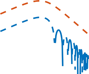
We check in figure 2 that the theoretical expressions (2.5), (2.6) and (2.9) well capture the longitudinal third-order structure function  $\langle \delta u_L^3 \rangle$ obtained from DNS in the inertial range, forcing scale and the no-flux range (large scales). In the inertial range, $\langle \delta u_L^3 \rangle$ scales as $r$, consistent with Kolmogorov's theory. In the no-flux range, $r > l_f$ with $l_f={\rm \pi} /k_f$ the forcing scale, as $r \rightarrow \infty$, the envelope of $\langle \delta u_L^3 \rangle$ scales as $r^{-2}$. Since we employed a triple periodic boundary condition, the theoretical and numerical results collapse to a range smaller than the domain size.

Figure 2. Theoretical solution (black) and results from DNS (blue) for the longitudinal third-order structure function  $\langle \delta u_L^3 \rangle$. (a) Exponential (type-I) forcing and (b) spherical shell (type-II) forcing. Solid lines represent the positive values and dashed lines represent the absolute value of the negative values.
In figure 3, we justify the decay rate with data from numerical simulations with six-mode forcing. In the no-flux range of figure 3, the spectrum has a  $k^2$ scaling, consistent with the absolute equilibrium. The longitudinal structure function, however, decays slowly as $r^{-2}$, the same as the other two forcing methods.

Figure 3. Results for forcing on six modes: ( $\pm k_f,0,0$), ( $0,\pm k_f,0$), ( $0,0,\pm k_f$). (a) Spectra and energy flux. (b) Third-order longitudinal structure function. Solid lines represent the positive values and dashed lines represent the absolute value of the negative values.
In figure 4, we present the p.d.f. of the normalized longitudinal velocity difference  $\mathcal {P}(\delta u_L / \langle \delta u_L^2 \rangle ^{1/2})$ with separations $r = 0.37$, $0.54$ and $0.70$, which correspond to the local extrema of the third-order structure function expression divided by the decaying rate $r^{-2}$ (cf. (2.10)) and are larger than the forcing scale $r_f = {\rm \pi}/k_f \approx 0.16$. The observed p.d.f.s are close to Gaussian distributions and we quantify the small departure from Gaussian using the odd parts of the p.d.f.s, which are shown in figure 5.

Figure 4. P.d.f.s of the normalized longitudinal velocity difference  $\mathcal {P}(\delta u_L / \langle \delta u_L^2 \rangle ^{1/2})$ at large scales (greater than the forcing scale $r_f \approx 0.16$). The black line represents the Gaussian distribution. Inset is the kurtosis of $\delta u_L / \langle \delta u_L^2 \rangle ^{1/2}$ at large separations $r$. (a) Exponential (type-I) and (b) spherical shell (type-II) forcing.

Figure 5. Odd part of the p.d.f. of normalized  $\delta u_L$ by $(\epsilon /k_f)^{1/3}$ at large separations and the absolute value of that divided by $r^{-2}$ (inset). (a) Exponential (type-I) and (b) spherical shell (type-II) forcing.
We justify the separate-of-variable form of the p.d.f. (2.11) in the insets of figure 5. When the p.d.f.s are normalized by  $g(k_f r)$, the curves collapse well, suggesting a universal $\mathcal {P}_0$. For the no-flux range (large scales), $g(k_f r) \sim r^{-2}$ for turbulence driven by type-I forcing. The $r$-dependence of $\mathcal {P}_{odd}$ representing the forcing effect, along with the universal of $\mathcal {P}_0$, indicates that the forcing dominates the dynamics of large scales. Thus, even though the non-Gaussian odd-part p.d.f. of the longitudinal velocity difference, $\mathcal {P}_{odd}$, is small, its slower decay rate than that of the forcing effect implies a strong interaction between large and small scales.
In figure 6, we justify the odd-order structure function expression (2.12) up to order 11 and find that  $C_{n} \approx -12 c^{n-3}$, with $c = 7$ and $c=6.6$ for the two forcing types, respectively. The convergence of the high-order structure functions is shown in the Appendix. This expression is further justified by the collapse of structure functions with different energy injection rates $\epsilon$ using the type-II forcing in figure 7.

Figure 6. Normalized high-odd-order structure function  $\langle \delta u_L^n \rangle / (\epsilon / k_f)^{n/3}/c^{n}$. (a) Exponential (type-I) forcing ( $c=7.0$) and (b) spherical shell (type-II) forcing ( $c=6.6$). Solid lines represent the positive values and dashed lines represent the absolute value of the negative values.

Figure 7. Normalized high-odd-order structure functions in numerical simulations with type-II forcing and varying energy injection rates.
4. Summary and discussion
In summary, we study the large-scale statistics of the forced 3-D homogeneous isotropic turbulence in the real separation space and find that the p.d.f.s of the longitudinal velocity difference are close to, but depart from, a Gaussian distribution. We measure this departure by the odd-part p.d.f.s. From the argument that large scales and forcing scale are well coupled, the large-scale dynamics ( $r > r_f$) are dominated by the forcing mechanism, where the odd-part p.d.f. of velocity difference $\mathcal {P}_{odd}$ for large separations can be written to a separate-variable form by separating the $r$-dependence, which leads to a universal $r$-dependence for odd-order structure functions. Even though the odd part of the p.d.f. has a smaller magnitude than the even part, the analytical solutions of the third-order structure function calculated from the KHM equation prove that the odd-part p.d.f. is non-zero. Also, when the forcing is localized in the spatial displacement space, e.g. exponentially decays as $r \rightarrow \infty$, the odd-order structure functions decay slowly following a power-law $r^{-2}$, implying that the long-range interaction between large and small scales is strong. Here we consider a localization that is more strict than the asymptotic locality which is used to study local energy transfer (cf. Eyink Reference Eyink2005).
Interestingly, this large-scale regime with a characteristic scale given by the forcing scale is conjugate to the inertial range of Kolmogorov's theory, where the characteristic scale is the separation. This discovery provides a more comprehensive understanding of turbulence because previous turbulence theory focuses on the inertial range, which cannot exist solely. Additionally, we need an understanding of dynamics at scales larger than the forcing scale. In free-decaying turbulence, when  $r \rightarrow \infty$, the longitudinal third-order structure function decays as $r^{-4}$ (Chapter 7 in Monin & Yaglom Reference Monin and Yaglom1975; Hosking & Schekochihin Reference Hosking and Schekochihin2023), which is weaker than the present forced turbulence situation. In our formulation, the forcing impact manifests itself by normalizing the velocity structure function using the energy injection rate and forcing scale, which is missing in the decaying turbulence.
An interesting implication is that if we have an observation of 3-D turbulence which cannot resolve the forcing scale, we can still know if there is unresolved energy injection, which could be a foundation for turbulence super-resolution. This implication is reasonable: even though there is no averaged upscale energy flux, the large-scale field needs to adjust accordingly to reach a statistically steady state with a forward cascade. From another perspective, if the 3-D turbulence is driven from an initially zero state, a transient energy flux to large scales must exist before reaching the statistically steady state, which links the small and large scales through energy injection and is remembered by the statistically steady state.
Acknowledgements
We greatly appreciate the anonymous reviewers for their comments, which significantly improved the manuscript.
Funding
This work was supported by the National Natural Science Foundation of China (M.D. and J.-H.X., grant nos. 92052102, 12272006, 42361144844; J.W., grant no. 12172161); and the Laoshan Laboratory (grant nos. LSKJ202202000, LSKJ202300100).
Declaration of interests
The authors report no conflict of interest.
Appendix. Convergence of the p.d.f. of the normalized longitudinal velocity difference
The p.d.f.s of the normalized longitudinal velocity difference  $\mathcal {P}(\delta u_L / \langle \delta u_L^2 \rangle ^{1/2})$ are well resolved as shown in figure 8 for the exponential (type-I) forcing and figure 9 for the spherical shell (type-II) forcing.

Figure 8.  $\mathcal {P}(\delta u_L / \langle \delta u_L^2 \rangle ^{1/2})$ multiplied by $\delta u_L^n / \langle \delta u_L^2 \rangle ^{n/2}$ ( $n=2,3,4,5,6,7,8,9,10,11$) at different scales for the exponential (type-I) forcing.

Figure 9.  $\mathcal {P}(\delta u_L / \langle \delta u_L^2 \rangle ^{1/2})$ multiplied by $\delta u_L^n / \langle \delta u_L^2 \rangle ^{n/2}$ ( $n=2,3,4,5,6,7,8,9,10,11$) at different scales for the spherical shell (type-II) forcing.


