


1. Introduction
Near-wall coherent structures are occasionally formed around the surface-mounted square cylinder subjected to oblique inflow (Thomas & Williams Reference Thomas and Williams1999; Ono, Tamura & Kataoka Reference Ono, Tamura and Kataoka2008); and regularly encountered in various engineering applications (building Cao et al. Reference Cao, Tamura, Zhou, Bao and Han2022, vehicles Zhang et al. Reference Zhang, Su, Tsubokura, Hu and Wang2022, aircraft Morris & Williamson Reference Morris and Williamson2020, high-speed trains Li et al. Reference Li, Chen, Liang, Liu and Xiong2021 and rough wall-bounded turbulent flow Nugroho, Hutchins & Monty Reference Nugroho, Hutchins and Monty2013; Chung et al. Reference Chung, Hutchins, Schultz and Flack2021). These structures include conical, horseshoe, arch-shaped vortices and Kelvin–Helmholtz instability because of the nonlinear interaction between the turbulent boundary layer and the obstacle. While severe structural damage and failure caused by the conical vortex were early reported and studied in civil engineering (Ginger & Letchford Reference Ginger and Letchford1993), the comprehensive study of those vortices and their interference to the reattachment and separation regions on obstacle's surfaces has seldomly been conducted. For simplicity, the oblique flow around surface-mounted square cylinder is considered as the typical idealization for capturing those vortex structures (Kawai & Nishimura Reference Kawai and Nishimura1996; Kawai Reference Kawai1997, Reference Kawai2002). In this paper, the characteristics of turbulent oblique flow past a surface-mounted square cylinder, including the mechanism of near-wall coherent vortex structures, their interference and spectral analysis are numerically carried out for comprehensive understanding of the underlying fluid mechanics.
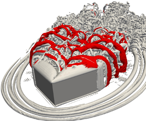
Figure 1(a) shows the schematic plot of coherent structures attached to a flat roof (conical vortex, Kelvin–Helmholtz instability), rear surface (arch-shaped vortex) and the ground (horseshoe vortex) when the turbulent oblique flow attacks the square cylinder roof. The cores of the conical and arch-shaped vortices are strongly correlated with the formation of Kelvin–Helmholtz (KH) and shear layer instabilities, respectively. As shown in figure 1(b), a pair of conical vortices occasionally evolves on the top surface, inducing the strong negative pressure suction along the square cylinder's windward edges. This pressure suction causes the switching of the conical vortices, producing unequal vortex cores of conical vortices at the square cylinder sides (shown in figure 1b i,iii). In addition, the suction also induces the flapping of the KH instability (shown in figure 1b ii,iv), thus interfering with the asymmetry of the arch-shaped vortex (shown in figure 1a). As listed in table 1, previous research ranges from semi-empirical theory, wind-tunnel experiments to large-eddy simulation; where the flow characteristics are classified into a relationship between conical vortex and negative pressure suction, effect of incident turbulent inflow and parapets on the pressure fluctuation and visualization of vortex structures. For the study related to vortex-suction correlation, Banks and Meroney (Banks & Meroney Reference Banks and Meroney2001a,Reference Banks and Meroneyb,Reference Banks and Meroneyc) utilized the quasi-steady theory to model the vortex flow mechanism to connect the increase in suction towards the roof corner. While Banks et al. (Reference Banks, Meroney, Sarkar, Zhao and Wu2000) performed the mean position and size of the corner vortices to prove no relationship between cross-stream vortex size and suction, the strong association between large peak suction and large conical vortex was reported by many works (Kind Reference Kind1986; Mehta et al. Reference Mehta, Levitan, Iverson and McDonald1992; Ginger & Letchford Reference Ginger and Letchford1993; Lin, Surry & Tieleman Reference Lin, Surry and Tieleman1995; Kawai Reference Kawai1997, Reference Kawai2002; Wu & Sarkar Reference Wu and Sarkar2006; Richards & Hoxey Reference Richards and Hoxey2008; Kozmar Reference Kozmar2020). Two spiral cores of conical vortices, developing from the roof corner, were observed by these authors. They alternately increase and decrease in size and vortex strengths, inducing the strong negative pressure fluctuation.

Figure 1. Illustration of coherent structures developed behind the surface-mounted square cylinder; (a) three-dimensional view; (b) the switching of the conical vortex and the flapping of the KH instability.
Table 1. Selected works of flow around surface-mounted square cylinders in oblique flows.
 $^{a}$SBL-smooth inflow, TBL – turbulent boundary layer, GTI – grid turbulent inflow. $^{b}$Theory: QST – quasi-steady theory, BLT – boundary layer theory. $^{c}$Experiment: WTE – wind-tunnel experiment, LLS – laser light sheet, LDA – laser Doppler anemometer, SDA – synchronized data acquisition, PWA – pulsed-wire anemometer, NICA – non-parametric independent component analysis. $^{d}$Simulation: LES – large-eddy simulation, LBE – lattice Boltzmann equation.
For the effect of incident turbulent inflow, Kawai (Reference Kawai1997, Reference Kawai2002) observed that the strength of conical vortices in smooth inflow is stronger than that in turbulent inflow. Also, the inclined angle of the conical vortex core to the windward edges in smooth inflow is larger than that in turbulent inflow. Otherwise, he also found that the strong conical vortex starts to form when the turbulent inflow approaches the roof at the angle of attack of  $\alpha =25^{\circ }$ to the windward edges. While Wu et al. (Reference Wu, Sarkar, Mehta and Zhao2001a,Reference Wu, Sarkar and Mehtab) pointed out the strong correlation of the vertical component of turbulent inflow with negative pressure suction, Castro & Robins (Reference Castro and Robins1977) elucidated that the turbulence inflow addition suppresses the strength of the conical vortex, thus reducing the streamwise velocity component. Marwood & Wood (Reference Marwood and Wood1997) investigated thoroughly the effect of lateral and vertical component turbulence on the roof pressure beneath conical vortices. They pointed out that the lateral wind component with large excursions causes the extremes in pressure.
For the pressure fluctuation observed on the roof conner, it is clarified that the switching phenomenon of the conical vortex induces the extremely negative pressure fluctuation (Kind Reference Kind1986; He et al. Reference He, Ruan, Mehta, Gilliam and Wu2007; Banks Reference Banks2013). Marwood & Wood (Reference Marwood and Wood1997) indicated that the instantaneous variation of the position of the conical vortex core significantly alters the pressure fluctuation. In particular, the extremely low pressure fluctuation occurs when the core is furthest from the windward edge and highest above the roof surface. Nishimura & Kawai (Reference Nishimura and Kawai2010) investigated the connection and interference between the switching conical vortex and wake vortex by adding a splitter plate onto the roof and in the wake. They found that the switching of the conical vortex disappeared when a splitter plate set in the wake. Hence, it is concluded that the wake vortex controls the conical vortex switching. Kawai & Nishimura (Reference Kawai and Nishimura1996) pointed out that the spiral rotation around the conical vortex core and its switching remarkably cause the travelling-wave-type suction fluctuations at the high and low frequency, respectively. Furthermore, the parapet configurations attached to the roof edge also have a significant impact on the high peak local suction (Baskaran & Stathopoulos Reference Baskaran and Stathopoulos1988; Bienkiewicz & Sun Reference Bienkiewicz and Sun1992).
While the pressure fluctuation on the top surface of the square cylinder is largely determined by the inlet turbulence intensity, parapet configuration, type of boundary layer and its thickness, the aspect ratio (AR) of the cylinder significantly alters the near-wake large-scale coherent structures (Sakamoto & Arie Reference Sakamoto and Arie1983; Kawamura et al. Reference Kawamura, Hiwada, Hibino, Mabuchi and Kumada1984; Okamoto & Sunabashiri Reference Okamoto and Sunabashiri1992; Sumner, Heseltine & Dansereau Reference Sumner, Heseltine and Dansereau2004). Pattenden, Turnock & Zhang (Reference Pattenden, Turnock and Zhang2005) found that the antisymmetrical Kármán and tip vortices transformed into an arch-shaped vortex as long as the AR is less than a critical value of  ${(h/w)_{cr}=2-6}$ (where $h$ and $w$ are the height and width of the square cylinder, respectively), depending on the boundary layer thickness and inflow turbulence intensity. While the intermittent occurrence of Kármán and arch-shaped vortices was observed in the near wake of the cylinder at AR $\approx (h/w)_{cr}$, an alternate Kármán vortex occurs along the square cylinder at AR $> (h/w)_{cr}$ (Okamoto & Sunabashiri Reference Okamoto and Sunabashiri1992). Hwang & Yang (Reference Hwang and Yang2004), Yakhot, Liu & Nikitin (Reference Yakhot, Liu and Nikitin2006) and Diaz-Daniel, Laizet & Vassilicos (Reference Diaz-Daniel, Laizet and Vassilicos2017) found only hairpin-like vortices in the wake of small AR square cylinders, often generated at low Reynolds numbers. These studies found that destabilizing the shear layer that detached from the square cylinder's top leading edge caused hairpin-like structures. Hearst, Gomit & Ganapathisubramani (Reference Hearst, Gomit and Ganapathisubramani2016) found that arch-shaped and tip vortices only apply to time-averaged flow in a wall-mounted cube ( ${\rm AR}=1$), whereas instantaneous wake structures, such as conical and KH vortices, are more complex and three-dimensional, causing highly fluctuating pressure suction on the top surface of a square cylinder ( ${\rm AR}=0.5$) (Kawai & Nishimura Reference Kawai and Nishimura1996; Thomas & Williams Reference Thomas and Williams1999; Kawai, Okuda & Ohashi Reference Kawai, Okuda and Ohashi2012). In addition, the instantaneous horseshoe and alternate Kármán vortices have not been reported in the literature for a square cylinder of AR $<2$ both experimentally and numerically.
Although the aforementioned studies have been conducted for many years using quasi-steady theory and wind-tunnel experiments, large-eddy simulations were rarely used to understand the detailed mechanism and characteristics of the near and far wake structures. A few studies have used large-eddy simulation to gain a thorough understanding of the conical vortex. He & Song (Reference He and Song1997) resolved the three-dimensional roof corner vortex, which produces large suction pressure on the roof surface, resulting in house roof damage. Thomas & Williams (Reference Thomas and Williams1999) successfully captured the three-dimensional near-wall and wake structures, including conical and KH vortices. In particular, the conical vortex dynamics, primary unsteady shedding of KH instability in the near wake, and the formation of a two-cell swirl pattern in the far wake, is investigated. Ono et al. (Reference Ono, Tamura and Kataoka2008) thoroughly investigated the switching conical vortex and its spiral motion. While the turbulence inflow was used by He & Song (Reference He and Song1997), the uniform and turbulent boundary layer inflows are utilized in the works of Thomas & Williams (Reference Thomas and Williams1999) and Ono et al. (Reference Ono, Tamura and Kataoka2008). It was pointed out that the coherent structures were well captured with and without the effect of the turbulent boundary layer except for the magnitude of the negative pressure peak near the suction edges.
To the best of the authors’ knowledge, the previous studies have been mainly performed for the effect of turbulent inflow and appearance of a conical vortex on the extremely negative pressure suction and fluctuation, while the comprehensive study of near-wall coherent structures, including KH and shear layer instability, horseshoe, arch-shaped and Kármán vortices, has not taken place. Particularly, three unclear points in the literature motivate this study, despite many attempts to describe the wake coherent structures of the square cylinder in oblique flow. The first is the incomplete identification of instantaneous near-wall structures related to horseshoe, arch-shaped, KH and Kármán vortices and their associations with the existence of a conical vortex and separated shear layer at AR  $<2$. The second is the previously weak visualization techniques (as listed in table 1) to capture these vortex structures. Therefore, taking the advantage of present direct numerical simulation (only large-eddy simulation (LES) performed in previous works), several advanced methods based on spectral analysis, vortex identifications and the critical-point concept are proposed in the present study; so that the small-to-large-scale coherent structures are comprehensibly distinguished with both instantaneous and time-averaged fields. The third is the effect of the Reynolds number on the near-wall and near-wake flow, specifically the vortex formation and its interference with the ground and square cylinder surfaces to crucially alter the reattachment and separation regions.
Naturally, this paper's originality is to deal with these three points. The uniform flow of oblique angle  $\alpha =45^{\circ }$ past a surface-mounted square cylinder of AR 0.5 is comprehensively studied at moderate Reynolds numbers of 3000 and 10 000. Without loss of generality, the uniform oblique inflow of $45^{\circ }$ and the cylinder's AR of 0.5 are followed from the work of Ono et al. (Reference Ono, Tamura and Kataoka2008) in the present study to sufficiently extract the complex flow features. Richards & Hoxey (Reference Richards and Hoxey2008) reported that the time-mean pressure coefficient on the separation corner of the square cylinder is lowest at $\alpha =45^{\circ }$. Although Saeedi, LePoudre & Wang (Reference Saeedi, LePoudre and Wang2014) observed nearly independent flow structures for Reynolds numbers greater than 2000, the effect of Reynolds number is significant in this study for manifesting distinct near-wall coherent vortex structures due to the interference of the approaching boundary layer and square cylinder's vortices. As listed in the literature review, the present Reynolds numbers are representative of higher Reynolds number cases and range within the previous investigations in order to capture the dominant flow physics.
The rest of this paper is organized as follows. Section 2 expresses the governing equations and numerical method based on the multiple-relaxation-time lattice Boltzmann equation combined with topology-confined block refinement. The flow configurations and computational set-up are discussed in § 3. Section 4 shows the results and discussions before the major conclusions summarized in § 5.
2. Methodology
2.1. Multiple-relaxation-time lattice Boltzmann equation
This present study uses an indoor code based on the mesoscopic approach known as the lattice Boltzmann equation (LBE). The LBE is a potential numerical method used in computational fluid dynamics (CFD) for turbulence, heat, multi-component and micro-flow applications (Succi Reference Succi2015). In contrast to typical CFD approaches (Higuera & Jiménez Reference Higuera and Jiménez1989; Higuera & Succi Reference Higuera and Succi1989; Higuera, Succi & Benzi Reference Higuera, Succi and Benzi1989), the Navier–Stokes equations (NSE) in the hydrodynamic limit are recovered using discretized particle distribution functions  $\varGamma$ (Ladd & Verberg Reference Ladd and Verberg2001). The LBE reconstructs the physical dynamics of viscous flows. By using the Bhatnagar–Gross–Krook (BGK) collision model (Chen & Doolen Reference Chen and Doolen1998), the LBE can be written as
 \begin{equation} \varGamma_i(\boldsymbol{x}+\boldsymbol{e}_i \Delta t,t+\Delta t)=\varGamma_i(\boldsymbol{x},t)-\omega(\varGamma_i(\boldsymbol{x},t)-\varGamma_i^{eq}(\boldsymbol{x},t)), \end{equation}
where  $\varGamma _i$, $\varGamma _i^{eq}$, $\boldsymbol {x}$, $\boldsymbol {e}_i$, $\Delta t$ and $\omega =1/\tau$ are the discrete-velocity distribution function, the local equilibrium distribution function, the corresponding physical location in space, particle velocity in the $i$th direction, time streaming step and relaxation frequency with a single relaxation time $\tau$. A general LBE procedure is divided into collision and streaming. While the collision process performs the right-hand side of (2.1), the streaming process accomplishes the full (2.1). In the current work, the D3Q27 (27 discrete velocities in 3 dimensions) particle velocity model is used; because it has been demonstrated that the LBE may meet the rotationally invariant flow condition in turbulence (Kang & Hassan Reference Kang and Hassan2013; Suga et al. Reference Suga, Kuwata, Takashima and Chikasue2015). The expression for this discretized velocity set is
 \begin{equation} \boldsymbol{e}_i= \begin{cases} 0, & i=0; \\ ({\pm} 1,0,0),(0, \pm 1,0),(0,0, \pm 1)c, & i=1,2,3,4,5,6; \\ ({\pm} 1,\pm 1,0),({\pm} 1, 0, \pm 1),(0,\pm 1, \pm 1)c, & i=7,8,\ldots,17,18; \\ ({\pm} 1,\pm 1,\pm 1)c, & i=19,20,\ldots,25,26, \\ \end{cases} \end{equation}
here,  $c$
$c$  $(=\Delta x/\Delta t)$ is taken as 1, where $\Delta x$ is the lattice spacing. For the D3Q27 model, the second-order local equilibrium distribution function is parametrized by the local values of density $\rho$ and flow velocity $\boldsymbol {u}$
 \begin{equation} \varGamma_i^{eq}(\boldsymbol{x}, t)=\rho w_i\left[1+\frac{\boldsymbol{e}_i \boldsymbol{\cdot} \boldsymbol{u}}{c_{s}^2}+\frac{\left(\boldsymbol{e}_i \boldsymbol{\cdot} \boldsymbol{u}\right)^2-\left(c_{s}|\boldsymbol{u}|\right)^2}{2 c_{s}^4}\right], \end{equation}
where  $w_0=8/27$, $w_i=2/27$ for $i=1-6$, $w_i=1/54$ for $i=7-18$, $w_i=1/216$ for $i=19-26$ and $c_{s}=c/\sqrt {3}$ represents the lattice sound speed.
Using the Chapman–Enskog analysis, the kinematic viscosity  $\nu$ associated with the single relaxation time $\tau$ as a connection between the LBE and the NSE (Huang Reference Huang2008), $\nu =c_{{s}}^2(\tau -0.5\Delta t)$. As a result, the results obtained from LBE can reveal values in macroscopic behaviour. However, the numerical stability of the BGK operator is limited when the value of the kinematic viscosity is sufficiently small. This issue often occurs in grid refinement attempts (discussed in the next section), cutting the single relaxation time (Wang Reference Wang2020). Based on the collision procedure (Lallemand & Luo Reference Lallemand and Luo2000), the multiple-relaxation-time (MRT) LBE is therefore performed to raise the free parameters of the relaxation time. In particular, the particle population relaxes in moment space instead of normal velocity space. Hence, (2.1) is replaced by
 \begin{equation} \varGamma_i(\boldsymbol{x}+\boldsymbol{e}_i \Delta t,t+\Delta t)=\varGamma_i(\boldsymbol{x},t)-\boldsymbol{M}^{{-}1}\boldsymbol{S}\left[m_{i}(\boldsymbol{x}, t)-m_{i}^{e q}(\boldsymbol{x}, t)\right]\Delta t, \end{equation}
where  $\boldsymbol {M}$, $\boldsymbol {S}$ and $m_i$ are the transformation matrix, collision matrix and moment space for distribution function $\varGamma$, respectively. In the current study, the matrices $\boldsymbol {M}$ and $\boldsymbol {S}$ are chosen from the results of the study of Suga et al. (Reference Suga, Kuwata, Takashima and Chikasue2015) for turbulent flow. In particular, $\boldsymbol {S}$ is a $27\times 27$ diagonal matrix with $s_{0-3}=0$, $s_{4}=1.54$, $s_{5-9}=1/(0.5+3\nu )$, $s_{10-12}=1.5$, $s_{13-15}=1.83$, $s_{16}=1.4$, $s_{17}=1.61$, $s_{18-22}=1.98$ and $s_{23-26}=1.74$. The formulation of transformation matrix $\boldsymbol {M}$ is established through the analysis of Dubois & Lallemand (Reference Dubois and Lallemand2011). A detailed performance of matrix $\boldsymbol {M}$ can be observed in Suga's study. All processes in the MRT method greatly improve the accuracy and stability of the single-relaxation-time lattice Boltzmann model.
Finally, macroscopic flow quantities (mass density  $\rho$, flow velocity $\boldsymbol {u}$ and intrinsic average pressure $p$) in the LBE framework can be obtained from moments of the particle distribution function
 \begin{equation} \rho(\boldsymbol{x}, t)=\sum_i \varGamma_i(\boldsymbol{x}, t), \quad \rho \boldsymbol{u}(\boldsymbol{x}, t)=\sum_i \boldsymbol{e}_i \varGamma_i(\boldsymbol{x}, t), \quad p(\boldsymbol{x}, t)=\rho(\boldsymbol{x}, t) c_{s}^2. \end{equation}
2.2. Boundary condition for bounded flows
In order to define the presence of rigid bodies in the fluid field, the input geometry uses the standard triangle language data, which provide the normal vector and vertex coordinates of triangular facets, defining the body surface as shown in figure 2(a). On the Cartesian mesh as depicted in figure 2(b), three types of cells are determined, including solid cells  $\boldsymbol {x}_s$, boundary cells $\boldsymbol {x_b}$ and fluid cells $\boldsymbol {x}_f$. Initially, the type of fluid cell is put in the full computational domain. The solid cells are then found using a fast ray-triangle intersection algorithm proposed by Möller & Trumbore (Reference Möller and Trumbore2005). Specifically, the exploration of solid cells is an inside/outside check of fluid cells with all triangular facets based on the ray parameterization. Then, the boundary cells $\boldsymbol {x}_b$ are the cells between the fluid cell and the solid cell. Finally, figure 2(c) demonstrates the three cell types after performing the ray-triangle intersection algorithm. At the boundary cell, the streaming process is performed to take into account the intentional neglect of lattice directions prevented by solid cells. This omission is compensated by the interpolated bounce-back (IBB) method (Bouzidi, Firdaouss & Lallemand Reference Bouzidi, Firdaouss and Lallemand2001) that satisfies the flow behaviour of second-order accuracy on the curved wall surface. The basic idea of the IBB method is to store the information of the intersection point between particle velocity vector $\boldsymbol {e}_i$ and the triangle facet. Determining the point of intersection is also performed by the ray-triangle intersection algorithm. According to Bouzidi et al. (Reference Bouzidi, Firdaouss and Lallemand2001), the reflection of a distribution function is predicted by linear interpolation. The a priori unknown bounced-back population is constructed from known populations at $\boldsymbol {x}_b$ and $\boldsymbol {x}_f$ as
 \begin{equation}
\varGamma_{\bar{i}}\left(\boldsymbol{x}_{b}, t+\Delta
t\right)=\left\{\begin{array}{@{}ll} 2 q
\varGamma_{i}^{+}\left(\boldsymbol{x}_{b}, t\right)+(1-2 q)
\varGamma_{i}^{+}\left(\boldsymbol{x}_{f}, t\right), & q
\leq \dfrac{1}{2},\\ \dfrac{1}{2 q}
\varGamma_{i}^{+}\left(\boldsymbol{x}_{b},
t\right)+\dfrac{2 q-1}{2 q}
\varGamma_{\bar{i}}^{+}\left(\boldsymbol{x}_{b}, t\right),
& q \geq \dfrac{1}{2}, \end{array}\right.
\end{equation}
\begin{equation}
\varGamma_{\bar{i}}\left(\boldsymbol{x}_{b}, t+\Delta
t\right)=\left\{\begin{array}{@{}ll} 2 q
\varGamma_{i}^{+}\left(\boldsymbol{x}_{b}, t\right)+(1-2 q)
\varGamma_{i}^{+}\left(\boldsymbol{x}_{f}, t\right), & q
\leq \dfrac{1}{2},\\ \dfrac{1}{2 q}
\varGamma_{i}^{+}\left(\boldsymbol{x}_{b},
t\right)+\dfrac{2 q-1}{2 q}
\varGamma_{\bar{i}}^{+}\left(\boldsymbol{x}_{b}, t\right),
& q \geq \dfrac{1}{2}, \end{array}\right.
\end{equation}
where  $q$ is the distance ratio between the distance $d$ measured from the boundary cell $\boldsymbol {x}_b$ to the intersection point and the magnitude of the discrete-velocity vector $\boldsymbol {e}_i$. As a result, $q=d/(|\boldsymbol {e}_i| \Delta t)\in [0,1]$ represents the reduced wall location information. Total fluid forces acting on the three-dimensional rigid body's surface ( $\boldsymbol {F}(F_x,F_y,F_z)$) are computed by the momentum exchange method (Chen et al. Reference Chen, Cai, Xia, Wang and Chen2013) on the boundary cell layer.

Figure 2. Interpolated bounce-back boundary condition (a); topology-confined block refinement with three levels (b); three partitions of solid cell, boundary cell and fluid cell (c).
2.3. Topology-confined block refinement
Based on the block-structured grids of Duong et al. (Reference Duong, Nguyen, Nguyen and Ngo2022), a framework of topology-confined block refinement is developed, as shown in figure 2(b). The computational domain is partitioned into areas of different grid sizes, called cube-shaped blocks. This spatial difference is characterized by an indicator called refinement level  $l$. Therefore, the mesh system is constructed with the value $l$ ranging from 0 to $l=m-1$, where $m$ is the number of the expected refinement level. The refinement level $l$ increases from the confined flow region near the solid bodies to far-field regions. In each block, the uniform Cartesian grid (cells) is used to store and solve the variables in the LBE. The efficiency and robustness of the management of the informational communication between refined and unrefined blocks are demonstrated in the numerical studies of Kamatsuchi (Reference Kamatsuchi2007) and Ishida, Takahashi & Nakahashi (Reference Ishida, Takahashi and Nakahashi2008). In each block, the index, coordinates, spatial size, cell number, grid refinement level and neighbouring block information are stored to provide detailed instructions within the cache environment for parallel computing. For parallelism, the block distribution on each grid refinement level is performed by a load-balanced linear distribution algorithm based on the space-filling curve theory (Bader Reference Bader2012). This procedure is implemented with the message passing interface technique, which is specially designed to function on parallel computing architectures. After distributing block data to each node, independent workloads are numerically performed by open multi-processing thread parallelization. Due to the space limitation, the interested readers are referred to the work of Duong et al. (Reference Duong, Nguyen, Nguyen and Ngo2022) for the detailed algorithm of topology-confined block refinement.
3. Numerical set-up
The numerical set-up is schematically shown in figure 3. A model of the surface-mounted square cylinder is shown in figure 3(a). The square cylinder width ( $w$) is used to normalize length scales and dimensions. The height of the square cylinder is $h=0.5w$, implying an AR of AR= $h/w=0.5$, which is identically considered in previous numerical and experimental studies (shown in table 1). Figure 3(b) shows the schematic of the computational domain and the definition of the coordinate system. The axis origin is located at the centre of the square cylinder's bottom surface. The streamwise ( $x$), spanwise ( $y$) and vertical ( $z$) dimensions are illustrated in the schematic by the red, dark blue and green arrows, respectively. The uniform free-stream velocity is set as $U_\infty$ at the inlet boundary. The lateral and upper boundaries of the domain are set to free-slip boundary conditions (Succi Reference Succi2001; Falcucci et al. Reference Falcucci, Aureli, Ubertini and Porfiri2011). The outlet boundary was set as the open boundary condition $\partial u/{\partial x}=0$. The no-slip boundary condition was applied on the bottom surface of the square cylinder using the half-way bounce-back method (Ladd Reference Ladd1994). The IBB method mentioned in § 2.2 is used to model the no-slip boundary condition on the square cylinder's surfaces.

Figure 3. Schematic of the computational domain; (a) three-dimensional view of the flow configuration; (b) set-up of the boundary condition enforcement; (c) symmetry plane view of the computational domain with the representation of topology-confined block-based grid; (d)  $x\unicode{x2013}y$ half-plane view of the computational domain with the representation of topology-confined block-based grid and the detailed cell distribution of confined regions; (e) grid system in $y\unicode{x2013}z$ planes of $x/w=0, 5$ and 12.5.
The computational domain size is selected as  $L_{up}+L_{do}=20w$, $W=15w$ and $H=10w$. The lateral length ( $W$) was reported as at least $10w$ for the sufficient accuracy by AIJ (2017). In this study, the current lateral length ( $15w$) is larger than the recommended value, thus ensuring the adequate lateral length of the computational domain. The present vertical length of $H=10w$ is contemplated based on the fact that the blockage effect of the top boundary on the separated shear layer developed above the top surface of the square cylinder should be sufficiently small. Furthermore, in the case of the set-up of the turbulent boundary layer at the inlet boundary, this vertical length should be adequately large to retain the streamwise development of the boundary layer. Cao et al. (Reference Cao, Tamura, Zhou, Bao and Han2022) proposed the minimum height ( $10w$) of the top boundary from the thickness of the turbulent boundary layer ( $\delta /y=20.1$). Therefore, in the present study, due to the set-up of uniform inflow (no turbulent boundary layer at the inlet), the vertical length of $10w$ is sufficiently large to capture the flow physics.
The spatial block distribution in the symmetry plane is shown in figure 3(c) while the  $x\unicode{x2013}y$ half-plane on the bottom surface of the square cylinder of $z/w=0$ and the $y\unicode{x2013}z$ planes are respectively shown in figure 3(d,e). The finer cell distribution is arranged in a confined region where the boundary layer is developed. Figure 3(c) shows $m=4$ levels where the cell sizes of $\varDelta$, $2\varDelta$, $4\varDelta$ and $8\varDelta$ represent levels $l=0,1,2,3$, respectively. The level $l=0$ is set up based on the fact that the finest resolution region should cover the development of the separated shear layers on the top and side surfaces of square cylinder. Hence, the grid generation strategy is based on three steps, including selection of block level, the dimensions of similar-level blocks in the computational domain, indication of uniform cell size (the cells are uniformly distributed in three directions of the cubed block). The total number of grids is computed as the multiplication between blocks and cells in one block.
In order to determine the minimum cell size, the thickness ( $\delta _B$) of the boundary layer developed on the cylinder's surfaces is calculated as $\delta _B=5.5 \times 0.5w/ \sqrt {Re_{0.5w}}$ based on the work of White (Reference White2006). In the present work, the maximum Reynolds number is $Re_w=U_{\infty } w/\nu =10\,000$, where $\nu$ is the kinematic viscosity. Five levels of grid refinement are employed, where the maximum level of finest resolution ( $\varDelta =w/256=0.0039w$ – the cell size) is confined to the square cylinder region. Therefore, the thickness of the boundary layer is $\delta _B=0.0388w$, thus expanding approximately 10 cells in the normal direction, which is identical to the resolution used in the work of Cao et al. (Reference Cao, Tamura, Zhou, Bao and Han2022). In other directions, the uniform cell size is applied as mentioned in § 2.3, indicating the $256 \times 256 \times 256$ cells distributed in a $1w \times 1w \times 1w$ volume of the surface-mounted square cylinder. The number of cells is also distributed for each cubic block, maintaining the block/cell ratio of $1/256=0.0039$ for three directions. This ratio is approximately equivalent to the range of $0.00285\unicode{x2013}0.0033$ investigated by Cao & Tamura (Reference Cao and Tamura2020) and Trias, Gorobets & Oliva (Reference Trias, Gorobets and Oliva2015), where the $0.00285$ and $0.0033$ ratios are on the lateral width and upper, lower and back walls of the square cylinder, respectively. Generally, the present resolution is higher than that of most numerical simulations or experimental measurements (PIV: particle image velocimetry) at the same Reynolds number, pointing out the total of 210 million cells utilized in this study. The examination of sufficient cell sizes is performed in § 3.1.
3.1. Verification and validation
First, we investigate the uniform flow past a square cylinder of lateral length ( $L^*=L/w=6$) at the angle of attack $\alpha =14^\circ$ to determine the sufficient grid resolution. The computational domain and the boundary conditions in this case are established based on the study of Oka & Ishihara (Reference Oka and Ishihara2009). Reynolds number is pointed as $10^4$; and topology-confined block refinement is used to generate a 5-level block system. For the space limitation, the computational domain is briefly described as ( $40w \times 15w \times 40w$). Here, we examine two different resolutions at the maximum level, including the coarse grid ( $\varDelta =w/256=0.0039w$) and the fine grid ( $\varDelta =w/400=0.0025w$), which correspond to approximately 210 and 330 million cells based on the above grid design (see figure 3), respectively. The time step $\Delta t^*=(\Delta t U_{\infty })/w$ is $5 \times 10^{-4}$, which is approximately equivalent to the time step of LES (Cao & Tamura Reference Cao and Tamura2020) and direct numerical simulation (DNS) (Trias et al. Reference Trias, Gorobets and Oliva2015).
Before comparing the present numerical results with references, the sufficient integration period of time for time-averaged values is investigated. The instantaneous, mean and root-mean-square aerodynamic coefficients exhibit temporal variation with normalized time of  $t^*=tU_\infty /w$, as shown in figure 4. The instantaneous drag and lift coefficients obtained by the fine grid are plotted in figure 4(a) with $t^*$ ranging from 0 to 1000. In figure 4(b), the mean drag in time is defined as $\bar {C}_D(t^*)= 1 /(t^*-t_{{start }}^*) \int _{t_{{start }}^*}^{t^*} C_D(t^*) d t^*$, where $t_{{start }}^*$ is the initial time at which the statistical average is calculated after the flow becomes statistically stationary ( $t_{{start }}^*=50$ in the present work). Root-mean-square drag in time is defined as $C_D^{\prime }(t^*)=1 /(t^*-t_{{start }}^*) \int _{t_{{start }}^*}^{t^*}[C_D(t^*)-\bar {C}_D(t^*)]^2 d t^*$. It is similar to mean and root-mean-square lift in time. To ensure clarity, the statistical values are scaled by those computed from $t_{{start }}^*$ until the end time (denoted by $t_{{end }}^*$); hence, the integration period of time is determined as $t_{{end }}^*-t_{{start}}^*$. The statistical values converged well from $t_{{end}}^*=680$ to $t_{{end}}^*=1000$ over the present simulation. In particular, the small vortex C at $t_{{end}}^*=1000$ is captured better than that at $t_{{end}}^*=500$ in the streamline contours. Figure 4(c,d) shows the comparison of the present $\bar {C}_p$ and $C_p^\prime$ along the square cylinder surfaces with those of Oka & Ishihara (Reference Oka and Ishihara2009); Nishimura & Taniike (Reference Nishimura and Taniike2000). The results of $t_{{end}}^*=1000$ collapse the references better than those of $t_{{end}}^*=500$. Therefore, the sufficient time-mean data are taken in the sampling range of $t^*=[50,1000]$, corresponding to approximately 95 Kármán vortex sheddings. The quantities for the pressure are defined as follows:
 \begin{equation} \bar{p}=\frac{1}{N}\sum_{1}^{N}p, \quad \bar{C}_p=\frac{\bar{p}-p_{\infty}}{0.5\rho_\infty U_\infty^2}, \quad C_p^\prime=\sqrt{\frac{1}{N}\sum_{1}^{N}\left(C_p-\bar{C}_p\right)^2}, \end{equation}
where  $p$,
$p$,  $p_{\infty }$, $\bar {p}$, $\bar {C}_p$ and $C_p^\prime$ are instantaneous pressure, reference pressure, time-mean pressure, time-mean pressure coefficient and root-mean-square pressure coefficient, respectively. Figure 5 shows the $\bar {C}_p$ and $C_p^\prime$ comparison of the present results with those of the references. As shown in figure 5(a,c), the $\bar {C}_p$ distributions of the present results along the cross-section of the square cylinder show a good agreement with those reported by Nishimura & Taniike (Reference Nishimura and Taniike2000) and Oka & Ishihara (Reference Oka and Ishihara2009). Along the BC surface the results obtained by coarse and fine grids approach that of Oka & Ishihara (Reference Oka and Ishihara2009). As depicted in figure 5(c,d), the present values of $C_p^\prime$ collapse those of Nishimura & Taniike (Reference Nishimura and Taniike2000) although the fine grid results show a better approach than the coarse results, especially along the BC and CD surfaces. Figure 6 depicts the time-mean streamline contour of the present results compared with those of the reference. As shown in the figure, the present positions of vortex centres behind the rear surfaces (A and B) and near the lower surface (C) agree well with those of the reference. The positions of vortex centres near the rear (E) and upper (F) surfaces resolved by the coarse grid are almost identical to those resolved by the fine grid; while the position of vortex centre (D) near the lower surface obtained by the fine grid tends to move upstream along the lower surface from that obtained by the coarse grid. For the comparison of hydrodynamic coefficients, the global hydrodynamic coefficients are computed as follows:
 \begin{gather} \bar{C}_{D}=\frac{1}{N}\sum_{1}^{N}\frac{F_x}{\tfrac{1}{2}\rho_\infty U_{\infty}^2 w}, \quad \bar{C}_{L}=\frac{1}{N}\sum_{1}^{N}\frac{F_y}{\tfrac{1}{2}\rho_\infty U_{\infty}^2 w}, \quad St=\frac{f w}{U_{\infty}}, \end{gather}
 \begin{gather} C_D^\prime=\sqrt{\frac{1}{N}\sum_{1}^{N}\left(C_D-\bar{C}_D\right)^2}, \quad C_L^\prime=\sqrt{\frac{1}{N}\sum_{1}^{N}\left(C_L-\bar{C}_L\right)^2}, \end{gather}
where  $C_{L}$, $C_{D}$, $\bar {C}_{L}$, $\bar {C}_{D}$, $C_L^\prime$, $C_D^\prime$ and $St$ are the instantaneous, time-mean and root-mean-squared lift and drag coefficients, and the Strouhal number, respectively. Here, $N$ represents the number of data instants. Table 2 indicates that the present results (time-averaged and root-mean-square values) obtained by the coarse and fine grids generally agree well with those of Oka & Ishihara (Reference Oka and Ishihara2009) (approximately ${<}5\,\%$); while a great scatter ( ${>}10\,\%$) is found among the experimental data (Igarashi Reference Igarashi1984; Nishimura & Taniike Reference Nishimura and Taniike2000). Specifically, Nishimura & Taniike (Reference Nishimura and Taniike2000) tested two cylinders with square cylinder aspect ratios of $AR_{sc}=8.3\unicode{x2013}16.7$ (where the $AR_{sc}$ is defined as the ratio of the spanwise length to the square cylinder width); and Igarashi (Reference Igarashi1984) performed the square cylinder of $AR_{sc}=3.75\unicode{x2013}10$. The discrepancy is due to the sensitivity to the experimental conditions, including $AR_{sc}$, end-plate condition, Reynolds number, free-stream turbulent intensity and blockage ratio. Therefore, the coarse grid is chosen for the rest of simulations to not only minimize the computational cost but also retain sufficient numerical accuracy.
Table 2. Comparison of time-mean hydrodynamic coefficients ( $\bar {C}_D$, $\bar {C}_L$, $St$,
$St$,  $C_D^\prime$ and $C_D^\prime$) between the present results and previous research for the uniform flow past the square cylinder at an angle of attack of $14^{\circ }$. The effect of sampling ranges of $t^* \in [50,1000]$ on these coefficients is shown corresponding to approximately 95 Kármán vortex sheddings.


Figure 4. Temporal and mean coefficients; (a) instantaneous drag and lift coefficients obtained by the fine grid of  $\varDelta =w/400$. The sampling range indicates the time range used for time-averaging quantities; (b) temporal convergence of aerodynamic coefficients; (c,d) comparison of $\bar {C}_p$ and $C_p^\prime$ along the square cylinder surfaces with references (Nishimura & Taniike Reference Nishimura and Taniike2000; Oka & Ishihara Reference Oka and Ishihara2009).

Figure 5. Comparison of the present results (with two different grids: coarse ( $\varDelta =w/256$) and fine ( $\varDelta =w/400$)) with references in the case of uniform flow past square cylinder at the angle of attack of $\alpha =14^\circ$; (a,c) the time-mean pressure coefficients; (b,d) the root-mean-square pressure coefficients.

Figure 6. Time-mean streamlines of uniform flow past square cylinder at the angle of attack of  $\alpha =14^\circ$; (a) the present result using coarse grid; (b) the present result using fine grid; (c) the reference result (Oka & Ishihara Reference Oka and Ishihara2009).
Second, we perform the simulation of uniform flow past a surface-mounted square cylinder of AR=1 at  $Re=10\,000$, and compare it with Castro & Robins (Reference Castro and Robins1977), using the grid resolution of $\Delta =w/256$. The computational domain is exactly identical to that mentioned in § 3. The time step $\Delta t^*$ is also selected as $5 \times 10^{-4}$. The time-mean data are taken in the sampling range of $200t^*$, corresponding to approximately 20 Kármán vortex sheddings. Figure 7 shows surface values of time-mean pressure coefficients, where red-filled nodes and continuous black lines stand for the reference and present results, respectively. As shown in the figure, at the corner edges, the present results deviate from those of experiment because of the different Reynolds numbers. Generally, the present results are in a good agreement with those of experiment. For the last validation, the simulation of uniform flow past a surface-mounted square cylinder of ${\rm AR}=0.5$ is performed at $Re=10\,000$. The set-up of the simulation is the same as the second one except for the AR of the square cylinder. The present results are shown in figure 8 to ensure the sufficient spatial and temporal resolutions based on the Kolmogorov length and time scales. In turbulent flow analysis, the Kolmogorov length and time scales are examined as dynamical parameters in space and time. According to Moin & Mahesh (Reference Moin and Mahesh1998) and Li et al. (Reference Li, Zhang, Dong and Abdullah2020), the closeness between the smallest resolved length and time scales and the Kolmogorov length and time scales determines the accuracy in resolving the fluctuations of turbulent flow. To confirm the validity of numerical computation, the present study investigated the ratio of the local grid size to the Kolmogorov length and time scales for both time-mean and instantaneous data fields. Here, the Kolmogorov length and time scales are respectively formulated as $\eta =(\nu ^3 / \epsilon )^{1/4}$ and $\tau =(\nu / \epsilon )^{1/2}$, with $\epsilon =(\nu /2)\overline {(\partial u_i'/\partial x_j^\ast +\partial u_j'/\partial x_i^\ast )^2}$ denoting the dissipation rate of turbulent energy per unit of cell volume, where $u_i^{'}$ is the fluctuating velocity.

Figure 7. Surface values of time-mean pressure coefficients where red-filled nodes and continuous black lines stand for the reference and present results, respectively.

Figure 8. (a) Schematic of the rectangular considered area is limited by the region of  $x/w=[-2,6]$, $y/w=[-2.5,2.5]$ and $z/w=[0,2]$. (b) Histogram of the ratio between the local grid size ( $\varDelta =\sqrt [3]{\Delta x^* \Delta y^* \Delta z^*}$) and the Kolmogorov length scale ( $\eta$), where the maximum and mean values of these are approximately $7.3$ and $0.6$. (c,d) Time-mean and instantaneous distributions of the ratio in the symmetry plane ( $y/w=0$) and $x\unicode{x2013}y$ plane ( $z/w=0.25$), respectively.
Figure 8(a) shows the schematic of two different planes of  $y/w=0$ and $z/w=0.25$ to show the distribution of $\varDelta /\eta$ in the regions near the square cylinder. A histogram of the ratio of the local grid size to the Kolmogorov length scale for this region is shown in figure 8(b). The results show that the maximum and time-mean values of these are approximately $7.3$ and $0.6$, respectively. In other research, Yakhot et al. (Reference Yakhot, Liu and Nikitin2006) and Saeedi et al. (Reference Saeedi, LePoudre and Wang2014) highlighted that the ratio of $\varDelta /\eta$ should be less than 5 in the critical regions containing the wakes behind the surface-mounted square cylinder at $Re=5610$ and 12000, respectively. Furthermore, the study conducted by Cao et al. (Reference Cao, Tamura, Zhou, Bao and Han2022) indicated that most of the turbulent kinematic energy is dissipated on a scale of $\varDelta /\eta =10$, which was the constraint used by most previous DNSs. As shown in figure 8(b), the present grid system has ensured that the ratio of $\varDelta /\eta$ is maintained below $7.3$. Both the time-mean (figure 8c) and instantaneous (figure 8d) contours of $\varDelta /\eta$ scale fall into the required range of $\varDelta /\eta =5-10$ discussed by previous investigators. In particular, the $\varDelta /\eta$ contour shown in the time-mean field is smaller than 5, while the $\varDelta /\eta$ contour greater than 5 in the instantaneous field is only $0.3\,\%$. Figure 9 shows a contour of the instantaneous and time-mean ratios of the computing time step ( $\Delta t^*$) to the Kolmogorov time scale ( $\tau$) for the near-cylinder region. The results show that the maximum and time-mean ratios are approximately $0.05$ and $0.015$, respectively. In other research, Li et al. (Reference Li, Zhang, Dong and Abdullah2020) highlighted that the time-mean ratio of $\Delta t^*/\tau$ should be less than 0.0205 to obtain the high-resolution results. Furthermore, as expressed in figure 9(a), $99.8\,\%$ of the computational domain shows the time-mean ratio of $\Delta t^*/\tau < 0.02$ while $0.2\,\%$ of the area confined to the upstream edges of square cylinder shows a time-mean ratio of $0.02 \le \Delta t^*/\tau \le 0.05$. For the instantaneous ratio shown in figure 9(b), the ratio of $0.02 \le \Delta t^*/\tau \le 0.05$ is confined to the boundary layer and side shear layers. Therefore, our time step and grid size are sufficiently small in order to capture the turbulent fluctuation in the present numerical simulations.

Figure 9. Contour of the ratio between the local time step ( $\Delta t^*$) and the Kolmogorov time scale ( $\tau$), where the maximum and mean values are approximately $0.05$ and $0.015$. (a,b) Depict the time-mean and instantaneous distributions of the ratio in the symmetry plane ( $y/w=0$) and $x\unicode{x2013}y$ plane ( $z/w=0.25$), respectively.
4. Results and discussions
This section focuses on the characteristics of instantaneous and time-mean coherent structures generated by a square cylinder of AR = 0.5 in an oblique flow of  $45^{\circ }$ at moderate Reynolds numbers of 3000 and 10 000 (based on $w$). Initially, the instantaneous fields are introduced to classify the coherent structures into five types, including horseshoe, hairpin, arch-shaped, conical, KH instability and Kármán vortices. Then, the spectrum analysis is performed to distinguish these flow structures in the frequency domain. Lastly, the time-mean fields are investigated, including the reconstruction of separated flow topologies based on critical-point concepts, characteristics of time-mean structures and Reynolds stress analysis.
4.1. Instantaneous field
4.1.1. Classification of instantaneous coherent structures
Figure 10 shows the instantaneous coherent structures developed behind the surface-mounted square cylinder in an oblique flow of  $45^{\circ }$ at $Re=3000$. Figure 10(a) clearly visualizes the horseshoe, hairpin and KH instability vortices by visualizing the contour of Q-criterion $Q=0.5(\|\overline {\boldsymbol {\varOmega }^*}^2\|-\|\overline {\boldsymbol {S}^*}^2\|)$, where $S^*_{ij}=0.5(\partial u_i^* / \partial x_j^*+ \partial u_j^* / \partial x_i^*$) and $\varOmega ^*_{ij}=0.5(\partial u_i^* / \partial x_j^*- \partial u_j^* / \partial x_i^*$). The horseshoe vortex is established in front of the square cylinder near the bottom surface-cylinder junction region. The horseshoe vortex formation is based on the fact that the shear development of the boundary layer from the bottom surface produces the vertical pressure gradient in front of the square cylinder. Hence, it causes the high momentum downflow stream towards the bottom surface; then the major deflection of this wall occurs in the upstream direction, forming the horseshoe vortex. In this study, the primary and secondary horseshoe vortices, observed due to the strong upstream flow, are developing around the square cylinder's junction region. The relative distance of the primary horseshoe vortex to the frontal surface of the $45^{\circ }$ square cylinder is closer than that of the $0^{\circ }$ square cylinder (Cao et al. Reference Cao, Tamura, Zhou, Bao and Han2022) and circular cylinder (Eckerle & Langston Reference Eckerle and Langston1987). That is because of the high favourable pressure gradient caused by the $45^{\circ }$-inclined front surfaces of the present square cylinder, generating the strong suction to the horseshoe vortex. The primary and secondary vortices remain stable at the distances of $x/w=3.5$ and $x/w=1.9$, respectively, thus indicating that the primary vortex is stronger than the secondary one. The KH vortices of C-shape are detected near the top and rear surfaces of the square cylinder. These vortices are formed due to the instability (breakup) of the shear layers that is highly dependent on the viscosity. Furthermore, it is interesting to note that the breakup of the secondary horseshoe vortex generates a hairpin-shaped vortex at $x/w=2.2$, including the hairpin tail (longitudinal structure) and the hairpin head (lateral structure). The hairpin head rolls up the primary horseshoe vortex as a result of the interaction between two counter-rotating vortex tubes (primary and secondary horseshoe vortices). Otherwise, the hairpin vortex observed in another downstream region is identical to that observed by Tufo et al. (Reference Tufo, Fischer, Papka and Szymanski1999).

Figure 10. Instantaneous coherent structures developed behind the surface-mounted square cylinder at  $Re=3000$; (a) isovalues of $Q=10$ represented by grey surfaces; (b) isovalues of $Q=10$ represented by grey surfaces while those of kinetic energy $0.5 \le E^*=0.5 {\boldsymbol {u}^*}^2\Delta x^*\Delta y^*\Delta z^*\le 0.9$ are represented by red surfaces; (c) isovalues of $Q = 10$ are represented by grey surfaces while positive and negative isovalues of the helicity $H^* = \boldsymbol {u}^{*} \boldsymbol {\cdot } \boldsymbol {\omega }^{*} = \pm 10$ are represented by yellow and blue surfaces, respectively.
Figure 10(b) shows the isovalues of  $Q=10$ represented by grey surfaces; and those of kinetic energy of $0.5 \le E^*=0.5 {\boldsymbol {u}^*}^2\Delta x^*\Delta y^*\Delta z^*\le 0.9$ are represented by red surfaces. Based on the kinetic energy contour, the formation of the arch-shaped vortex is captured at the distance $x/w=1.5$ downstream. Initially, the C-shape KH instability vortices are asymmetrically formed near two rear surfaces of the square cylinder and develop their size downstream. Then, when the size of two C-shape vortices is sufficiently large, the two vortices combine into one arch-shaped vortex. Hence, the leg and arch parts of the vortex are formed by the instability of the shear layer separated from the rear and top surfaces of the square cylinder, respectively. Time-averaged experimental data (Ahmed, Ramm & Faltin Reference Ahmed, Ramm and Faltin1984; Hucho & Sovran Reference Hucho and Sovran1993; Lienhart & Becker Reference Lienhart and Becker2003; Liu et al. Reference Liu, Zhang, Zhang and Zhou2021) reported C-shaped vortices attached to two side edges of the Ahmed model in oblique flow of $\alpha =30^{\circ }$. However, for $\alpha > 30^{\circ }$, the wake development of C-shaped vortices was not observed. One significant observation in the present result is that, at $\alpha = 45^{\circ }$, the C-shaped KH vortices remain at some distance downstream and then develop into a three-dimensional (3-D) arch-shaped vortex before transforming into complex 3-D structures in the intermediate wake. Otherwise, the current work clearly visualizes the M-shaped instantaneous arch vortex, which is similar to those found by Wang & Zhou (Reference Wang and Zhou2009) and Zhu et al. (Reference Zhu, Wang, Wang and Wang2017) in the case of a circular cylinder. Furthermore, in the context of a square cylinder, the current 3-D arch-shaped vortex has a more distinct shape compared with the 2-D arch-shaped vortex discovered by Kawai et al. (Reference Kawai, Okuda and Ohashi2012).
Figure 10(c) shows isovalues of  $Q = 10$ represented by grey surfaces; and the positive and negative isovalues of the helicity $H^* = \boldsymbol {u}^{*} \boldsymbol {\cdot } \boldsymbol {\omega }^{*} = \pm 10$ are represented by yellow and blue surfaces, respectively. The yellow and blue surfaces also signify the clockwise and counterclockwise rotations of the vortex structures, respectively. As shown in the figure, the counter-rotating conical vortex tubes are observed above the top surface of the square cylinder. The clockwise-rotating conical vortex (yellow surface) shows its broken part because of the KH instability. He et al. (Reference He, Ruan, Mehta, Gilliam and Wu2007) and Banks et al. (Reference Banks, Meroney, Sarkar, Zhao and Wu2000) utilized visualization techniques to capture the instantaneous position of conical vortex cores in the selected cross-sections along the streamwise direction while Marwood & Wood (Reference Marwood and Wood1997), Kawai (Reference Kawai1997) and Kawai (Reference Kawai2002) employed the velocity vector plot technique to visualize the time-mean core and reattachment points. The latest numerical model by Ono et al. (Reference Ono, Tamura and Kataoka2008) for a square cylinder in $45^{\circ }$ oblique flow used particle trace, velocity vector and streamwise vorticity techniques to extract the instantaneous core. One important observation in the present result is that the contour of helicity can clearly detect not only the instantaneous core but also the vortex rotation of the conical vortex. Moreover, the helicity contour reconfirms that the primary and secondary horseshoe vortices on each lateral side are counter-rotating in the downstream region (only co-rotating in the near frontal surface); and the hairpin vortex tail and head are also counter-rotating. In the region behind the rear surfaces of the square cylinder, the vortex structures are three-dimensional.
Figure 11 shows the time histories of the pressure coefficients at four probe points located near the upstream edges of the square cylinder at  $Re=10\,000$. The pressure values recorded at probe points $a$ and $c$ are nearly the same, similarly at probe points $b$ and $d$. This means that the conical vortex develops its size at the corner of the cylinder's top surface. The switching of the conical vortex occurs at $t^*=115, 135$ and 152, inducing a high jump in the local pressure coefficient ranging from $-$1.2 to $-$0.5. This observation is generally similar to that observed by the numerical method of Ono et al. (Reference Ono, Tamura and Kataoka2008) and experiments of Kawai (Reference Kawai2002) and Nishimura & Kawai (Reference Nishimura and Kawai2010). The only difference is that the asymmetric feature is observed in the present result for the instantaneous pressure coefficients at two symmetric probe points with respect to the wake centreline. The identical asymmetry is also observed in the data obtained by other numerical simulations (Ono et al. Reference Ono, Tamura and Kataoka2008) while the symmetry is observed using an experimental method (Kawai Reference Kawai2002). It can be noticed that the asymmetry might be caused by the limitation of the present computational domain length ( $20w$). Nishimura & Kawai (Reference Nishimura and Kawai2010) tried to see the main factor of the wake vortices causing the conical vortex switching by using a splitter plate on the roof surface or in the wake of the square cylinder. They observed that the switching of the conical vortex still occurs with a splitter plate on the roof surface while it does not appear with a splitter plate in the wake, implying a strong effect of wake vortices on the switching. For this interesting point, we will discuss more details of the major factor related to wake vortex structures in the following subsections.

Figure 11. Time histories of pressure coefficients at four probe points (a–d) located near the upstream edges of the square cylinder at  $Re=10\,000$.
4.1.2. Dependence of Reynolds number
Figure 12 depicts the instantaneous coherent structures and pressure coefficient contours on the top surface of a square cylinder at  $Re=3000$ and 10 000 during a switching process of a conical vortex. While figure 12(a,c) shows the switching process of a conical vortex at $Re =3000$, figure 12(b,d) shows the switching process of a conical vortex at $Re =10\,000$. The coherent structures around the square cylinder are highly changeable because of the Reynolds number effect, although the switching process of a conical vortex occurs independently of the change of Reynolds number. The highly negative pressure suction region is observed to be switched on upstream sides of the top surface of the square cylinder. The appearance of the conical vortex is identical to that observed by numerical and experimental methods (Kawai Reference Kawai1997, Reference Kawai2002; Ono et al. Reference Ono, Tamura and Kataoka2008). However, this appearance was detected based on the time history record of the pressure coefficient along the upstream edges of a square cylinder's top surface while the present observation is made clearer using the Q-criterion contour of the flow field. The switching of the conical vortex is highly correlated with the Kármán vortex shedding behind the square cylinder due to the Reynolds number effect. This Kármán vortex is induced by the arch-shaped vortex deformation, occasionally developing from side to side of the square cylinder. At higher Reynolds number, the pressure suction region spreads along two upstream sides of the cylinder's top surface (shown in figure 12b,d); while it spreads along one upstream side at lower Reynolds number (shown in figure 12a,c). That is because the KH instability forms during the development of a conical vortex at higher Reynolds number ( $Re=10\,000$), thus causing the waving reattachment lines. Therefore, it can be noted that the conical vortex pair strongly attaches to the top surface at $Re =10\,000$ while it weakly attaches to the top surface at $Re =3000$. Furthermore, due to the Reynolds number effect, the angle between the reattachment line and the upstream edge of the square cylinder at $Re=3000$ ( $28.4^{\circ }$) is larger than that at $Re=10\,000$ ( $20.6^{\circ }$). The large pressure suction on the top surface of the square cylinder caused by a conical vortex was previously detected using extraction of the time-mean and root-mean-square pressure coefficient and reattachment lines by Kawai & Nishimura (Reference Kawai and Nishimura1996), Kawai (Reference Kawai1997), Marwood & Wood (Reference Marwood and Wood1997), Kawai (Reference Kawai2002) and Banks (Reference Banks2013). They found that the reattachment line is inclined relative to the square cylinder's edge from $19.5^{\circ }$ to $28.5^{\circ }$ while the vortex core centreline is inclined from $12^{\circ }$ to $14^{\circ }$ to the square cylinder's edge. Therefore, our results fall into the observed range of references. In addition, the distinct observation in the present work is that the variation of the Reynolds number plays a crucial role in determining the inclination of conical vortex reattachment, showing the inverse proportion of the Reynolds number increase to the inclination.

Figure 12. Instantaneous coherent structures and pressure coefficient contour on the top surface of square cylinder at  $Re=3000$ and 10 000 during a switching process of a conical vortex; (a,c) the switching process of conical vortex at $Re =3000$ (jfm.2023re3000); (b,d) the switching process of conical vortex at $Re =10\,000$ (jfm.2023re10000). Panels show (a) $Re =3000$, $t^*=195$, (b) $Re =10\,000$, $t^*=125$, (c) $Re =3000$, $t^*=236$, (d) $Re =10\,000$, $t^*=145$.
At  $Re=3000$, the arch-shaped vortex is asymmetrical and controlled by the pair of conical vortices. In particular, as shown in figure 12(a), when the conical vortex attaches to the top surface (shown by the reattachment line), the smaller part of the arch-shaped vortex is observed. In an opposite manner, when the conical vortex detaches from the top surface, the larger part of arch-shaped vortex is observed. A similar observation is obtained at higher Reynolds number (shown in figure 12b). Hence, it is fair to note that the formation of the arch-shaped vortex does not depend on the Reynolds number as long as the conical vortex develops on the top surface of the square cylinder. Otherwise, the instability of the horseshoe vortex in the front and wake of the square cylinder occurs at a higher Reynolds number of $Re=10\,000$. The primary and secondary horseshoe vortices are observed at $Re =3000$ while the primary horseshoe vortex is clearly detected at $Re =10\,000$ (the secondary horseshoe vortex is weakly formed).
4.1.3. Undulation of Kelvin–Helmholtz instability
Figure 13 expresses the instantaneous pressure coefficients at two probe points located along the side shear layer developed behind the rear surfaces of the square cylinder at  $Re=3000$. Figure 13(a) shows the instantaneous pressure coefficients at two probe points (A and B) located on the $x\unicode{x2013}y$ plane ( $z/w=0.5$) while figure 13(b) depicts the contour of the pressure coefficient at four instants of $t^*=195, 236, 277$ and 319. As shown in figure 13(a), the instantaneous pressure coefficients denote the sway process of the shear layer, being related to the Kármán vortex shedding. The sway of the shear layer of low frequency starts from $t^*=175$, where the signal of KH instability of relatively higher frequency appears intermittently with larger amplitude. The visualization of the shear layer sway and the development of KH instability along the shear layers (red and yellow curved lines) are clearly depicted in figure 13(b). During the sway process, the KH instability is signified by small portions of negative pressure coefficient along the shear layers. These KH vortices move downstream with the free-stream velocity and join with the 3-D vortices in the far field. The signals of these low and high frequency vortices are transformed to elucidate the quantitative details of these coherent motions. The identical occurrences of the KH instability in the cylinder's wake are characterized by other investigators of 2-D circular and square cylinders (Prasad & Williamson Reference Prasad and Williamson1997; Lander et al. Reference Lander, Moore, Letchford and Amitay2018; Liu, Hamed & Chamorro Reference Liu, Hamed and Chamorro2018) and surface-mounted square cylinders (Thomas & Williams Reference Thomas and Williams1999). Furthermore, it is interesting to note that, when the shear layer sways itself from up to down (based on top view), the negative pressure suction region caused by the conical vortex also switches itself from one to another upstream side of the square cylinder. This also reconfirms the strong correlation between the switching of the conical vortex and the Kármán vortex shedding, as observed in figure 12. Nishimura & Kawai (Reference Nishimura and Kawai2010) described the interaction between the conical vortex and Kármán vortex in the wake although Bienkiewicz & Sun (Reference Bienkiewicz and Sun1992) and Kawai & Nishimura (Reference Kawai and Nishimura1996) insisted that the conical vortex switching appeared irregularly without the effect of wake vortices. Therefore, the present scrutiny reconfirms the work of Nishimura & Kawai (Reference Nishimura and Kawai2010), revealing the identical frequency of conical vortex and Kármán vortex sheddings.

Figure 13. Instantaneous pressure coefficients at two probe points located along the side shear layer developed behind the rear surfaces of the square cylinder at  $Re=3000$; (a) instantaneous pressure coefficients at two probe points (A and B) located on the $x\unicode{x2013}y$ plane ( $z/w=0.5$); (b) the contour of pressure coefficient at four instants of $t^*=195, 236, 277$ and 319.
Figure 14 shows the flapping process of KH instability developed on the top surface of a square cylinder where the left-hand side and right-hand side columns indicate the downward and upward flapping, respectively. As shown in figure 14(a,c), two shear layers, developed from the leading and trailing edges of the square cylinder, are observed in flapping-down process. In this stage, the shear layers are strongly suctioned by the low pressure region distributed on the cylinder's surface. In figure 14(e), the separated shear layer remains laminar in the range between the separation point near the leading edge of  $x/w=0$ and $x/w=0.25$. The instability region is shown in the range between $x/w=0.25$ and $x/w=1.5$. During this process, the KH vortex starts to shed from the laminar shear layer at $x/w=0.25$ because of the amplification of the disturbance. Then, it evolves and gets larger in size at $x/w=0.45$. The KH vortex is stretched and interacts with other discrete vortices at $x/w=0.8$. The stretching process includes vortex splitting, forming the transition region of the KH instability. In the flapping-down process (shown in figure 14b–d), only one shear layer, developed from the leading edge of the square cylinder, is observed. At this stage, the shear layer undulates upward because of the higher surface pressure distribution compared with the downward process. Due to the upward undulation of the shear layer, the KH vortex starts to shed from the laminar shear layer at $x/w=0$ because of the amplification of the disturbance. Then, it evolves with larger deformation at $x/w=0.65$. The KH vortex is stretched and interacts with other discrete vortices at $x/w=1.2$ by diffusing vorticity, causing vortex breakdown into random eddies. Generally, the KH vortices on the top surface of the surface-mounted square cylinder are identical with those observed by Brun et al. (Reference Brun, Aubrun, Goossens and Ravier2008) for a 2-D square cylinder at $Re=2000$. However, in this study, it is interesting to note that the position, where the KH vortex starts to shed, tends to move upstream along the shear layer during the flapping-up process compared with that during the flapping-down process.

Figure 14. Flapping process of KH instability developed on the top surface of square cylinder at  $Re=3000$ where the left-hand side and right-hand side columns indicate downward and upward flapping, respectively; (a,b) the contour of velocity magnitude; (c,d) the contour of vorticity magnitude; (e,f) the contour of Q-criterion.
Figure 15 analyses the spectra ( $\phi$) of streamwise velocity fluctuations ( $u^{'}=u^{*}-\tilde {u}^{*}$, where $\tilde {u}^{*}$ stands for the moving-averaged streamwise velocity) at nine probe points located along the core of the conical vortex developed on the top surface of the square cylinder at $Re =3000$. As shown in the figure, the frequencies of von Kármán vortex shedding ( $f_{VK}$) and KH instability ( $f_{KH}$) are clearly observed at six locations from point 1 to point 6, where only the sign of KH instability is identified at points 7, 8 and 9. At the separation point close to the leading edge of the square cylinder (point 1), the signature of the von Kármán vortex is unclear while it is obvious at points 2, 3, 4, 5 and 6, where two peaks of $f_{VK}$ and $0.5f_{VK}$ are detected. From point 3 to point 9, two signatures of KH vortices of $f_{KH}$ and $0.5f_{KH}$ are also observed, revealing the occurrence of vortex pairing. The frequencies $f_{KH}$ and $0.5f_{KH}$ are remarkably noticeable at points 1, 2 and 3, signifying the development of KH vortices along the conical vortex on the top surface of the square cylinder. The frequencies $f_{KH}$ and $0.5f_{KH}$ at points of 4 to 9 are signified by the KH vortices shed from the shear layer of the rear surfaces of the square cylinder. At points 7, 8 and 9, the energy spectrum cascade of the flow approaches the $k^{-5/2}$ slope. The present results of $f_{KH}$ and $0.5f_{KH}$ are identical at all probe points along the shear layer while those spectral frequencies are lower with an increase in distance along the shear layer, as observed by Lander et al. (Reference Lander, Moore, Letchford and Amitay2018). The change of spectral frequencies is because of the reduction of convection velocity of the KH vortices in the shear layer of the 2-D square cylinder; and the reverse flow between the cylinder’s surface and the shear layer also reduces the convection velocity. However, the reverse flow is neglected in the present 3-D square cylinder because of the occurrence of strong conical vortex tubes on the cylinder's top surface, as observed in figure 10(c).

Figure 15. Spectra of streamwise velocity fluctuations ( $\phi$) at nine probe points located along the core of the conical vortex developed on the top surface of the square cylinder at $Re =3000$.
Figure 16 expresses the scaling of the ratio of KH and von Kármán frequencies ( $f_{KH}/f_{VK}$) as a function of Reynolds number ( $Re$). The continuous and dash-dotted lines are the scaling models of square and circular cylinders proposed by Lander et al. (Reference Lander, Moore, Letchford and Amitay2018) and Prasad & Williamson (Reference Prasad and Williamson1997), respectively. The frequency ratio scaling of the square and circular cylinders, represented by the power-law relations, are $f_{KH}/f_{VK}=0.18Re^{0.6}$ and $f_{KH}/f_{VK}=0.0235Re^{0.67}$, respectively. Right-pointing triangle is the LES data of Brun et al. (Reference Brun, Aubrun, Goossens and Ravier2008). Square is the DNS data of Trias et al. (Reference Trias, Gorobets and Oliva2015). Circle is the laser Doppler velocimetry data of Lander et al. (Reference Lander, Moore, Letchford and Amitay2018). Diamond is the present LBE data at $Re =3000$ and 10 000 where the inset depicts the spectra of three components of the velocity fluctuation at probe point 2 $(-0.598w,-0.046w,0.02w)$ at $Re =10\,000$. The present results show a good agreement with the power-law relation of the square cylinder. It is interesting to note that the energy spectrum approaches the $k^{-5/3}$ slope of Kolmogorov's similarity hypothesis at $Re =10\,000$; while the $k^{-5/2}$ slope is obtained at $Re =3000$. The higher inclination of the energy spectra at higher Reynolds number is correlated with the vortex structures formed behind the square cylinder. As can be seen in figure 12, the larger coherent structures (KH instability and arch-shaped vortex) occur in the wake at $Re=3000$ while smaller structures appear at $Re=10\,000$. Hence, it is fair to note that the smaller coherent structures demonstrate the more inclined energy spectrum slope of Kolmogorov's similarity hypothesis, reconfirming the present finding of a Reynolds number effect discussed in the previous subsection. As reported by Prasad & Williamson (Reference Prasad and Williamson1997), Brun et al. (Reference Brun, Aubrun, Goossens and Ravier2008) and Liu et al. (Reference Liu, Hamed and Chamorro2018), the frequency of Kármán vortex shedding slightly increases in the range of $10^3 < Re <5.4*10^4$ for the case of a 2-D circular cylinder while it remains nearly unchanged for the case of a 2-D square cylinder in the range of $1.5*10^4 < Re <7.4*10^4$ (Lander et al. Reference Lander, Moore, Letchford and Amitay2018). Therefore, it primarily depends on the kinematic viscosity of the flow. In the present work, the frequency of Kármán vortex shedding at $Re=10\,000$ (figure 16) is slightly larger than that at $Re=3000$ (figure 15), following the trend obtained by the circular cylinder references. Therefore, it should be noted that the Kármán vortex shedding frequency is not controlled by the spanwise length of the 2-D circular cylinder or the package of vortices (arch-shaped, conical and KH) of a low-AR surface-mounted square cylinder.

Figure 16. Ratio scaling of KH frequency and von Kármán frequency,  $f_{KH}/f_{VK}$ as a function of Reynolds number ( $Re$). The continuous and dash-dotted lines are the scaling models of square and circular cylinders proposed by Lander et al. (Reference Lander, Moore, Letchford and Amitay2018) and Prasad & Williamson (Reference Prasad and Williamson1997), respectively. Right-pointing triangle ( $\triangleright$) is the numerical data of Brun et al. (Reference Brun, Aubrun, Goossens and Ravier2008). Square ( $\square$) is the numerical DNS data of Trias et al. (Reference Trias, Gorobets and Oliva2015). Circle ( $\circ$) is the experimental data of Lander et al. (Reference Lander, Moore, Letchford and Amitay2018). Diamond ( $\blacklozenge$) is the present data, where the inset depicts the spectra of three velocity fluctuation components at probe point 2 $(-0.598w,-0.046w,0.02w)$ at $Re =10\,000$.
4.1.4. Association of coherent structures with flow separation
It was thoroughly discussed in previous sections that the large pressure suction is generated along the upstream edges close to a roof corner of the square cylinder. This local suction is induced by a pair of conical vortices on the roof resulting from flow separation from these edges. Otherwise, the horseshoe, arch-shaped, KH, hairpin and Kármán vortices were also observed. In this section, we will extract the association and correlation with flow separation of these coherent structures. Figure 17 shows the correlation of a conical and KH vortex with a horseshoe vortex at  $Re =3000$. Instantaneous contours of vorticity magnitude ( $|\boldsymbol {\omega }|$) and velocity vector distribution on $y\unicode{x2013}z$ planes of $x/w=0$ and $x/w=0.9$ are expressed during a switching process of conical vortices at $t^{*}=195$ and $t^{*}=236$. As shown in the figure, the flow pattern changed suddenly from $t^*=195$ to $t^*=236$ and vice versa in the $y\unicode{x2013}z$ plane of $x/w=0$, as the left and right parts of the conical vortex core grew and decayed alternately. The conical vortex part showing oppositely rotating spiral cores attaches closely to the roof surface, corresponding to the maximum suction on the roof directly underneath the conical vortex. This phenomenon is identical to what was observed by Kawai (Reference Kawai1997) and Taniguchi & Taniike (Reference Taniguchi and Taniike1996). The difference in the current study is that we recognize the conical vortex by contour of vorticity magnitude, which is better than the wind-tunnel visualization in the previous research. In $y\unicode{x2013}z$ plane of $x/w=0.9$, the conical vortex core continuously elongates downstream and drives the roof's KH vortex to roll in the clockwise direction, generating the re-entrant part of the arch-shaped vortex expressed in figure 17(a), which was similarly observed by Kawai et al. (Reference Kawai, Okuda and Ohashi2012). However, this study shows that the arch-shaped vortex is formed by the KH vortices from the roof and side surfaces (as also observed in figure 10a). Moreover, during the switching process, the leg parts of the arch-shaped vortex alternately grew and decayed in vorticity magnitude. Simultaneously, the primary horseshoe vortex rolls toward the side surface of the square cylinder ( $0.67w$) near the stronger vorticity part. Meanwhile, the opposite primary horseshoe vortex was driven away ( $0.8w$) from the side surface of the square cylinder near the weaker vorticity part as a result of the sway process of the side shear layers (figure 13). It was oppositely observed in figure 17(b). Therefore, it demonstrates the strong correlation of KH vortex with horseshoe vortex.

Figure 17. Correlation of conical and KH vortex with horseshoe vortex at  $Re =3000$. Instantaneous contours of vorticity magnitude ( $|\boldsymbol {\omega }|$) and velocity vector distribution on $y\unicode{x2013}z$ planes of $x/w=0$ and $x/w=0.9$ are expressed during a switching process of conical vortices at $t^{*}=195$ (a) and $t^{*}=236$ (b).
Figure 18 clearly shows not only the association of coherent structures with flow separation, but also the crucial role of the Kármán vortex at  $Re=10\,000$ in affecting the oscillating frequency of KH, conical and horseshoe vortex structures. Two probe points A and B are respectively located near the side shear layer and horseshoe vortex to capture the dominant frequencies around these vortices. As seen in figure 18(a), the dominant frequencies at probe point A include the Kármán ( $f_{VK}$) and KH ( $f_{KH}$) frequencies; meanwhile those at probe point B involve the Kármán and hairpin frequencies ( $f_H$ shown in figure 18d). It is interesting to note that the hairpin frequency is lower than the KH frequency; while the Kármán frequency dominates both the side shear layer and the horseshoe vortex. The detection of $f_{KH}$ in the present study is also similar to that observed by Kawai & Nishimura (Reference Kawai and Nishimura1996). Figure 18(b,c) expresses the sway process of the horseshoe vortex at $Re=10\,000$ due to the dominance of the Kármán vortex, which is generated due to the instability of the arch-shaped vortex shown in figure 18(d). The sway of the present horseshoe vortex is in agreement with the observations of Pattenden et al. (Reference Pattenden, Turnock and Zhang2005) and Krajnović (Reference Krajnović2011) for a circular cylinder.

Figure 18. Association of coherent structures at  $Re =10\,000$; (a) spectra of streamwise velocity fluctuations ( $\phi$) at two probe points A (located near the side separated shear layer) and B (located near horseshoe vortex); (b,c) sway process corresponding to one Kármán vortex shedding; (d) instantaneous coherent structures developed behind the surface-mounted square cylinder at $Re=10\,000$ with isovalues of $Q=10$ coloured by velocity magnitude.
4.2. Time-averaged field
4.2.1. Flow separation
To comprehensively interpret the 3-D complex separation of oblique flow past a surface-mounted square cylinder, critical-point theory is employed to obtain the logical elucidation of this complex flow in a time-mean sense. That is because the instantaneous surface flow pattern is identical to the time-mean surface flow pattern when the shear layer is close to the surface (Cao, Tamura & Kawai Reference Cao, Tamura and Kawai2019). The theory distinguishes the critical points, where the indeterminate streamlines or skin-friction lines are obtained from high-resolution numerical simulation or experiment (Délery Reference Délery2001). Accordingly, the flow topology is introduced by critical points, detachment/reattachment lines, separation/reattachment surfaces and topological rules to describe consistently the complex flow separation. Figure 19 shows classification of the critical point in the  $p$–
$p$– $q$ chart (defined by the eigenvalues $\lambda _1$ and $\lambda _2$ of the velocity derivative tensor, $F_{ij}=\partial \tau _{wi}/\partial x_{j}$, where $\tau _{wi}$ stands for surface shear stress), reproduced following Délery (Reference Délery2001). The purple-filled points represent unstable and stable foci and the centre while the green- and red-filled points stand for isotropic, attachment and separation nodes and saddle points, respectively. In this study, foci, nodes, saddle points, half-saddle points, half-node points, attachment lines and separation lines are respectively denoted by $F$,
$F$,  $N$,
$N$,  $S$,
$S$,  $S^{'}$, $N^{'}$, $(A)$ and $(S)$. These critical points satisfy the topological basic rules (Délery Reference Délery2013) as follows:
 \begin{equation} \left(\sum N+ \frac{1}{2} \sum N^{'}\right) - \left(\sum S+ \frac{1}{2} \sum S^{'}\right) = 1-n. \end{equation}
For a simply connected domain,  $n = 1$; for a doubly connected domain, $n = 2$.

Figure 19. Classification of critical point in the  $p$–
$p$– $q$ chart, reproduced following Délery (Reference Délery2001). The purple-filled points represent unstable and stable foci and the centre while the green- and red-filled points stand for isotropic, attachment and separation nodes and saddle points, respectively.
Figure 20 shows the separated flow topologies projected on the  $x\unicode{x2013}y$ planes of $z/w = 0.05, 0.25$ and $0.5$. Figure 20(a i,b i,c i) shows the surface flow patterns of the present simulation results, visualizing the pseudo-streamlines with respect to the velocity vector; figure 20(a ii,b ii,c ii) reconstructs the flow topology based on critical-point concepts from figure 20(a i,b i,c i). The colour shows the contour of the time-mean pressure coefficient ranging from $-1$ to 1.4. Figure 20(a) shows the topology of the bottom-surface flow, represented by foci ( $F_1$ and $F_2$), saddle points ( $S_1$, $S_2$, $S_3$ and $S_4$), half-saddle points ( $S_1^{'}$, $S_2^{'}$ and $S_3^{'}$), nodes ( $N_1$ and $N_2$), half-node point ( $N_1^{'}$), separation lines ( $(S_1)$, $(S_2)$, $(S_3)$, $(S_4)$ and $(S_5)$) and attachment line $(A)$. Generally, the present result of $S_3$, $S_4$, $N_1$ and $S_1$ agrees well with that obtained by Thomas & Williams (Reference Thomas and Williams1999). Furthermore, all critical points of the bottom-surface flow in this study satisfy the topological constraint of a doubly connected domain (4.1), such as ( $\sum N+ \tfrac {1}{2} \sum N^{'}) - (\sum S+ \tfrac {1}{2} \sum S^{'})=-1$, where $\sum N=4$, $\sum N^{'}=1$, $\sum S=4$ and $\sum S^{'}=3$. The free-stream flow approaches and diverges from the separation line ( $S_1$), where the divergence point is the saddle point $S_1$. The separation line ( $S_1$) is the contact line of the secondary horseshoe vortex with the bottom surface. This vortex originates from the saddle point $S_1$, surrounds the square cylinder and extends downstream before entering the free-stream flow. The attachment line ( $A$) starts from the node $N_1$ and emanates around the square cylinder, forming the contact line of the primary horseshoe vortex with the bottom surface. Similarly, the primary horseshoe vortex also spreads around the square cylinder, and proceeds downstream before entering the free-stream flow. In the wake region, the shear flows (separated from the half-saddle points $S_2^{'}$ and $S_3^{'}$) and the reversed flows (started from the half-node point $N_1^{'}$) spin towards the symmetrical foci $F_1$ and $F_2$. These two foci $F_1$ and $F_2$ are isolated by separation lines $(S_3)$ and $(S_4)$, passing through the saddle points $S_3$ and $S_4$, respectively. In other bluff body studies, one saddle and two focus points are regularly observed in the time-mean wake while two saddle and two focus points are identified in the present study.

Figure 20. The separated flow topologies projected on the  $x\unicode{x2013}y$ planes: (a) $z/w = 0.05$; (b) $z/w = 0.25$; (c) $z/w = 0.5$. Figures (a i,b i,c i) show the surface flow patterns of the present simulation results, visualizing the pseudo-streamlines with respect to the velocity vector; figures (a ii,b ii,c ii) reconstruct the flow topology based on critical-point concepts from the left-hand side figures. The colour shows the contour of the time-mean pressure coefficient ranging from $-1$ to 1.4.
Figure 20(b) expresses the flow topology in the  $x\unicode{x2013}y$ plane of $z/w=0.25$, represented by foci ( $F_1$, $F_2$, $F_3$ and $F_4$), saddle point $S_1$, half-saddle points ( $S_1^{'}$, $S_2^{'}$, $S_3^{'}$, $S_4^{'}$, $S_5^{'}$, $S_6^{'}$, $S_7^{'}$ and $S_8^{'}$), separation lines ( $(S_1)$ and $(S_2)$). All critical points also satisfy the topological constraint of a doubly connected domain, where $\sum N=4$, $\sum N^{'}=0$, $\sum S=1$ and $\sum S^{'}=8$. The symmetrical foci $F_1$ and $F_2$ are formed by the reversed flows started from saddle points $S_6^{'}$ and $S_7^{'}$, respectively. The vortex foci $F_3$ and $F_4$ are symmetrical and isolated by the separation line $(S_2)$ of the saddle point $S_1$, which is identical to other bluff body studies. Figure 20(c) expresses the flow topology in the $x\unicode{x2013}y$ plane of $z/w=0.5$, represented by foci ( $F_1$ and $F_2$), node $N_1$, half-saddle points ( $S_1^{'}$, $S_2^{'}$, $S_3^{'}$, $S_4^{'}$, $S_5^{'}$, $S_6^{'}$, $S_7^{'}$ and $S_8^{'}$). All critical points also satisfy the topological constraint of a doubly connected domain, where $\sum N=3$, $\sum N^{'}=0$, $\sum S=0$ and $\sum S^{'}=8$. The formation of two symmetrical foci $F_1$ and $F_2$ is different from that in the middle plane of $z/w=0.25$. In particular, the reversed flows started from the saddle point $S_6^{'}$ and node $N_1$ roll themselves towards $F_1$; and similarly to $F_2$.
Figure 21 expresses the flow topology in the  $x\unicode{x2013}z$ plane of $y/w=0$, represented by foci ( $F_1$, $F_2$, $F_3$, $F_4$ and $F_5$), saddle point $S_1$, half-saddle points ( $S_1^{'}$, $S_2^{'}$, $S_3^{'}$, $S_4^{'}$, $S_5^{'}$, $S_6^{'}$, $S_7^{'}$, $S_8^{'}$, $S_9^{'}$ and $S_{10}^{'}$). All critical points also satisfy the topological constraint of a doubly connected domain, where $\sum N=5$, $\sum N^{'}=0$, $\sum S=1$ and $\sum S^{'}=10$. In the cylinder–surface junction region of the square cylinder, the foci $F_1$ and $F_2$ represent the primary and secondary horseshoe vortices. On the top surface, the focus $F_3$ is the vortex bubble that arises near the leading edge because of the reversed flow starting from the saddle point $S_6^{'}$. In the wake region, the shear layer developed from the trailing edge of the top surface (half-saddle point $S_{7}^{'}$) proceeds downstream and rolls itself towards the attachment region, originating from the half-saddle point $S_{10}^{'}$. The large recirculation zone of the node centre $F_5$ is manifested between the separated shear layer and small recirculation zone of node centre $F_4$ in the junction region.

Figure 21. The separated flow topology projected on the  $x\unicode{x2013}z$ plane of $y/w = 0$; (a) the surface flow pattern of the present simulation results, visualizing the pseudo-streamlines with respect to the velocity vector; (b) the reconstruction of the flow topology based on critical-point concepts. The colour shows the contour of the time-mean pressure coefficient ranging from $-1$ to 1.4.
Figure 22 depicts the flow topologies on the top and leeward surfaces of the square cylinder which are reproduced from the surface streamline contours. As shown in figure 22(a), the symmetrical separation lines of  $(S_1)$ and $(S_2)$, originating from the separation point near the upstream corner point of the square cylinder signify the detachment of the conical vortex from the top surface while the attachment line $(A_1)$ is the contact line of the conical vortex with the top surface. Therefore, the conical vortex manifests itself between the separation and attachment lines, forming the symmetrical conical vortices at two regions segregated by the attachment line $(A_1)$. The separation line $(S_2)$ continuously extends on the leeward surface of the square cylinder, as shown in figure 22(b). The $(S_2)$ line is finally prevented by attaching the separation node point $N_2$. Otherwise, the attachment node point $N_1$ is observed to firmly connect with two saddle points $S_1$ and $S_2$. The reversed flows from right to left caused by the adverse pressure gradient are isolated by the separation line $(S_5)$ of the saddle point $S_2$. The saddle point $S_3$ is observed in the cylinder–surface junction region with its two separation lines $(S_6)$ and $(S_7)$.

Figure 22. Reproduction of flow topologies on the square cylinder surfaces from the present results of surface streamline contours: (a) top-surface flow topologies; (b) leeward surface flow topologies.
4.2.2. Time-mean coherent structures
Figure 23 expresses time-mean streamline contours with critical points in the symmetry plane in the junction region near the front cylinder surface and compares the present results with those obtained by Jenssen et al. (Reference Jenssen, Schanderl, Strobl, Unglehrt and Manhart2021). In the reference data, the Reynolds number was investigated at  $Re_D=39\,000$ (where $D$ is the diameter of circular cylinder). In the present results, the blue and red contours represent the regions of the negative (called wall-parallel jet) and positive streamwise velocity, respectively. As shown in figure 23(c), these regions are isolated by the black layer, where the streamwise velocity approaches zero. Wall-parallel jet region is formed by the downflow intruding into the bottom surface at half-saddle point $S_3$, then deflecting in the upstream direction, and finally penetrating the bottom surface until the half-saddle point $N_1$. In the reference results shown in figure 23(a,b), a part of the downflow is redirected to the cylinder front surface at node point $V_3$, which is not observed in the present study. The primary and secondary horseshoe vortex centres at foci $V_1$ and $V_2$ are observed in the present study while only a primary horseshoe vortex centre is detected in the reference. The present location of $V_1$ ( $x/w+0.205=-0.621$) is closer to the cylinder surface than that of the reference ( $x/D=-0.73$, as shown in figure 23b). That is because the favourable pressure gradient at upstream surfaces of $45^{\circ }$ square cylinder is larger than those of a circular cylinder (Baker Reference Baker1980; Pattenden et al. Reference Pattenden, Turnock and Zhang2005; Jenssen et al. Reference Jenssen, Schanderl, Strobl, Unglehrt and Manhart2021). Although the present thickness of the wall-parallel jet is higher than that of the reference because of the occurrence of $V_2$, the present location of $N_1$ ( $x/w+0.205=-1.09$) is identical to that of the reference ( $x/D=-1.1$, as shown in figure 23b).

Figure 23. Time-mean streamline contours with critical points in the symmetry plane in the junction region near the front cylinder surface; (a,b) particle image velocimetry and LES data of a circular cylinder (Jenssen et al. Reference Jenssen, Schanderl, Strobl, Unglehrt and Manhart2021); (c) present results of a square cylinder where the blue and red contours represent the negative (wall-parallel jet) and positive time-mean streamwise velocities, respectively.
Figure 24 depicts 3-D separation flow visualization in the top-surface region projected on seven  $z\unicode{x2013}y$ planes of $x/w$ ranging from $-$0.6 to 0.9. According to the discussion of the development of a symmetrical conical vortex on the top surface of a square cylinder in figure 22(a), seven planes are arranged to capture the development of one time-mean conical vortex on a half-side of the square cylinder's top surface. Each plane visualizes the contour of vorticity magnitude with respect to the pseudo-streamlines. Starting from the separation point, the conical vortex core expands its size with an increase in $x/w$, forming the conical vortex core, as also observed in figure 10(c). From $x/w=-0.6$ to $x/w=0.25$ the conical vortex still attaches the top surface while it moves upwards and rolls in the counterclockwise direction at $x/w=0.6$ and 0.9 because of the sway of the shear layer on the leeward surface. It reconfirms the strong correlation between the sway of the shear layer and the switching of the conical vortex discussed in figure 13. Otherwise, the reattachment line is observed to be more inclined from the upstream edge than the conical vortex core, which is similar to other references (Kawai & Nishimura Reference Kawai and Nishimura1996; Kawai Reference Kawai1997; Marwood & Wood Reference Marwood and Wood1997; Kawai Reference Kawai2002; Banks Reference Banks2013). The 3-D coordinate of the conical vortex core is extracted by figure 25, where the attachment of the conical vortex is clearly shown on the top surface. While the upstream portion creates and time-mean angle of $26.4^{\circ }$ to the upstream edge, the downstream portion of the conical vortex core proceeds aloft when this vortex travels out from the top surface.

Figure 24. Three-dimensional separation flow visualization in the top-surface region projected on seven  $z\unicode{x2013}y$ planes of $x/w$ ranging from $-$0.6 to 0.9. Each plane visualizes the contour of vorticity magnitude with respect to the pseudo-streamlines.

Figure 25. The conical vortex core above the top surface of the square cylinder.
The aloft part of the conical vortices continuously travels downstream and establishes the arch-shaped vortex, as observed in figure 26. The arch-shaped vortex and its deformation projected on the  $y\unicode{x2013}z$ planes of $x/w$ ranging from 0.75 to 2 is visualized, where left-hand side figures indicate the streamwise time-mean vorticity contours; and right-hand side figure shows the Q-criterion contour of $Q=10$. The horseshoe, side shear layer and conical vortices are clearly captured around the square cylinder while the base streamwise vortex pair is also detected in the moderate wake of the square cylinder. The tip and base vortices are categorized as the streamwise counter-rotating vortices that always occur in the near- and moderate- wake of the 3-D square cylinder (da Silva et al. Reference da Silva, Chakravarty, Sumner and Bergstrom2020; Cao et al. Reference Cao, Tamura, Zhou, Bao and Han2022). In this study, the tip vortex pair is not observed due to the small cylinder AR of 0.5. In the in-plane flows at $x/w=0.75$, the symmetrical arch-shaped vortices are established by two counter-rotating parts, including clockwise (blue contours) and counterclockwise (yellow contours) parts. Each part contains a vortex head and tail. In particular, the upward flows travel vertically from the bottom surface of $z/w=0$ to $z/w=0.45$, then emanate in the opposite transverse directions, thus forming the symmetrical arch-shaped vortices. The development of these vortices is driven by the conical vortices. As a result, the head vortex starts to split from its tail at $x/w=0.9$ because of the aloft part of the conical vortex core. These vortices are partly split at $x/w=1.2$, and they are fully broken into the 3-D vortex structures at $x/w=2$. Simultaneously, the downflow caused by the downwash roll of the shear layer from the top surface (observed in figure 21) occurs to manifest the base vortices. Therefore, it is interesting to note that the formation of the base vortex is highly correlated to the streamwise termination of the arch-shaped vortex.

Figure 26. Visualization of arch-shaped vortex and its deformation projected on  $y\unicode{x2013}z$ planes of $x/w$ ranging from 0.75 to 2; (a–d) indicate the streamwise time-mean vorticity contours; (e) shows the Q-criterion contour of $Q=10$.
The arch-shaped vortex core in the wake of the square cylinder is shown in figure 27, where the vortex centres of the core are coordinated from the streamline contours shown in figures 20 and 21. The arch-shaped vortex was rooted by two foci on the  $x\unicode{x2013}y$ plane near the bottom surface. Furthermore, the inclination of the arch-shaped vortex core is clearly observed and driven by the aloft part of the conical vortex (as seen in figure 24), which connects to the sway of the separated shear layer from the square cylinder side (as seen in figure 13). The attachment of the downwash flow of the conical vortex pair at the attachment line $(A_1)$ (depicted in figure 22a) exhibits the re-entrance of the arch-shaped vortex, which is identical to that observed by Kawai et al. (Reference Kawai, Okuda and Ohashi2012).

Figure 27. The arch-shaped vortex core in the wake of square cylinder.
4.2.3. Reynolds stresses
To understand the detailed interaction between the coherent structures around the square cylinder and boundary layer on the bottom surface, the transport of turbulent fluctuations is investigated in this section. The Reynolds stresses connecting directly to the turbulence intensity is discussed, including normal ( $\overline {u^{'}u^{'}}$, $\overline {v^{'}v^{'}}$ and $\overline {w^{'}w^{'}}$) and shear ( $\overline {u^{'}v^{'}}$ and $\overline {w^{'}u^{'}}$) stresses. That is because the Reynolds stress component of $\overline {v^{'}w^{'}}$ is nearly zero due to statistical symmetry. The present examination of the Reynolds stress will shed some light on the characteristics of wake coherent structures in time-mean fluctuation sense, including primary and secondary horseshoe vortices (denoted as PHS and SHS, respectively), side shear layer (SSL), rolled shear layer (RSL), arch-shaped vortex (ASV) and base vortex (BV). Figure 28 depicts the Reynolds normal stress projected on the $x\unicode{x2013}y$ planes of $z/w=0.05, 0.25$ and 0.5 while figure 28(a,d,g) shows the spanwise-averaged Reynolds normal stress of $\overline {u^{'}u^{'}}$, (b,e,h) and (c,f,i) show the transverse- and vertically averaged Reynolds normal stresses of $\overline {v^{'}v^{'}}$ and $\overline {w^{'}w^{'}}$, respectively. For the distribution of $\overline {u^{'}u^{'}}$, at the bottom surface of $z/w=0.05$, the signature of the side shear layer, primary and secondary horseshoe vortices are clearly marked. At $z/w=0.25$, the PHS and SHS disappear while the SSL is intensified together with the existence of the arch-shaped vortex. At $z/w=0.5$, the SSL and ASV are greatly escalated. For the distribution of $\overline {v^{'}v^{'}}$, the attachment region (observed in figure 21) is intensively signified at the $z/w=0.05$ because of the rolled shear layer separated from the cylinder's top surface. The intensity of the shear layer is reduced at $z/w=0.25$ and 0.5, which is opposite to the distribution of $\overline {w^{'}w^{'}}$.

Figure 28. Averaged Reynolds normal stress projected on  $x\unicode{x2013}y$ planes of $z/w=0.05, 0.25$ and 0.5; (a,d,g) show the spanwise-averaged Reynolds normal stress of $\overline {u^{'}u^{'}}$; (b,e,h) show the transverse-averaged Reynolds normal stress of $\overline {v^{'}v^{'}}$; (c,f,i) show the vertically averaged Reynolds normal stress of $\overline {w^{'}w^{'}}$.
Figure 29 shows the time-averaged Reynolds shear stress projected on the  $x\unicode{x2013}y$ planes of $z/w=0.05, 0.25$ and 0.5. While the left-hand side column shows the Reynolds shear stress of $\overline {u^{'}v^{'}}$, the right-hand side column expresses the Reynolds normal stress of $\overline {w^{'}u^{'}}$. For the distribution of $\overline {u^{'}v^{'}}$, the PHS, SSL and BV are clearly marked at $z/w=0.05$ while the colour contours mean counter rotations. The counter-rotating base vortices reconfirm the identical observation to the previous studies (da Silva et al. Reference da Silva, Chakravarty, Sumner and Bergstrom2020; Cao et al. Reference Cao, Tamura, Zhou, Bao and Han2022). At $z/w=0.25$, only the SSL is intensively magnified while the ASV and SSL are simultaneously detected at $z/w=0.5$. For the distribution of $\overline {w^{'}u^{'}}$, the ASV is clearly observed at $z/w=0.25$ and greatly intensified at $z/w=0.5$ while it is weakly captured at the bottom surface. Figure 30 depicts averaged Reynolds normal and shear stresses projected on the symmetry plane. While the streamwise-, transverse- and vertical-averaged Reynolds normal stresses are respectively shown in figures 30(a), 30(b) and 30(c), the averaged Reynolds shear stress of $\overline {w^{'}u^{'}}$ is expressed in figure 30(d). The rolled shear layers are well captured in the distributions of $\overline {u^{'}u^{'}}$, $\overline {w^{'}w^{'}}$ and $\overline {w^{'}u^{'}}$ while the high intensity of $\overline {v^{'}v^{'}}$ is concentrated on the attachment region. Especially, the highest intensity of $\overline {v^{'}v^{'}}$ is around the half-saddle point $S_{10}^{'}$, as observed in figure 21.

Figure 29. Averaged Reynolds shear stress projected on  $x\unicode{x2013}y$ planes $z/w=0.05, 0.25$, and 0.5; (a,c,e) show the Reynolds shear stress of $\overline {u^{'}v^{'}}$; (b,d,f) show the Reynolds normal stress of $\overline {w^{'}u^{'}}$.

Figure 30. Averaged Reynolds normal and shear stresses projected on the symmetry plane of  $y/w=0$. (a) Averaged Reynolds normal stress $\overline {u^{'}u^{'}}$. (b) Averaged Reynolds normal stress $\overline {v^{'}v^{'}}$. (c) Averaged Reynolds normal stress $\overline {w^{'}w^{'}}$. (d) Averaged Reynolds shear stress $\overline {w^{'}u^{'}}$.
5. Conclusions
The complete near-wall coherent structures around a 3-D surface-mounted square cylinder of  ${\rm AR} =0.5$ in an oblique uniform flow of $\alpha = 45^{\circ }$ have been comprehensively investigated for the first time by using LBE combined with block-structured topology-confined mesh refinement and a fast ray-triangle intersection algorithm. A very high resolution Cartesian mesh ( $256 \times 256 \times 256$ cells for a volume of $1w \times 1w \times 1w$) is utilized to capture the detailed characteristics of coherent structures and the small-scale flow separation at moderate Reynolds numbers of 3000 and 10 000. The critical-point concept was employed to describe the reasonable and compatible topologies of flow separation around and on the square cylinder's surfaces. The detailed findings of the present study on the coherent structures with the topological description are encapsulated as follows.
The large-scale horseshoe vortices (primary and secondary) at two notable foci are frequently observed in the junction region in front of the square cylinder. The wall-parallel jet region developed on the bottom surface is formed by the downflow intruding into the bottom surface at the half-saddle point, then deflecting in the upstream direction and finally penetrating the bottom surface until the half-saddle point. The present location of primary horseshoe vortex centres is closer to the square cylinder surface than that of the reference. That is because the favourable pressure gradient at upstream surfaces of a  $45^{\circ }$ square cylinder is larger than those of a circular cylinder and a $0^{\circ }$ square cylinder.
A pair of conical vortices is usually observed on the cylinder's top surface. In the instantaneous field, the conical vortices switch themselves on two cylinder sides, where the switching frequency is identical to that of the sway of the side shear layer. In the time-mean field, the conical vortex core consists of two segments. While the upstream segment is attached to the cylinder surface, the downstream segment moves upwards because of the sway of the side shear layer. The undulation of the KH instability is observed in the instantaneous development of the conical vortex and side shear layer. The KH frequency is smaller than the Kármán frequency, which connects to the sway of the side shear layer. The scalings of the ratio of the KH and von Kármán frequencies show a good agreement with the power-law relation ( $f_{KH}/f_{VK}=0.18Re^{0.6}$) of the square cylinder proposed by Lander et al. (Reference Lander, Moore, Letchford and Amitay2018).
The large-scale arch-shaped vortex is often detected in the intermediate wake region of the square cylinder, involving two inter-connected portions, such as a leg portion separated from the side leeward surfaces and a head portion rolled up from the top surface. The leg portion of the arch-shaped vortex was rooted by two foci on the bottom-surface plane near the bottom surface. The inclination of the arch-shaped vortex core is driven by the aloft part of the conical vortex, connecting to the sway of the separated shear layer from the square cylinder side. The re-entrance of the arch-shaped vortex is exhibited by the attachment of the downwash flow of the conical vortex pair at the attachment line. The streamwise counter-rotating base vortices observed close to bottom surface are formed because of the downwash roll of the shear layer from the top surface. The formation of the base vortex is highly correlated to the streamwise termination of the arch-shaped vortex.
Supplementary movies
Supplementary movies are available at https://doi.org/10.1017/jfm.2024.554.
Acknowledgements
We are deeply grateful to all the anonymous reviewers for their invaluable, detailed and informative suggestions and comments on the drafts of this article. The authors are extremely grateful to Mr K. Uchibori for technical support and fruitful discussions regarding the numerical methods.
Funding
This research is funded by Vietnam National Foundation for Science and Technology Development (NAFOSTED) under grant number 107.03-2021.37.
Declaration of interests
The authors report no conflict of interest.


