


1. Introduction
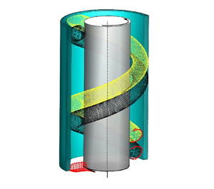
Spiral Poiseuille (SP) flow is the fluid motion developing within an annular geometry under the combined action of an axial pressure gradient and the relative cylinder rotation. A schematic representation of the resulting flow is shown in figure 1(a), which gives an idea of the spatial evolution of the rolls in the gap region at moderate rotation rates and pressure gradients. This set-up is relevant to several industrial applications, such as bearing lubrication or sealing and cooling of rotating machineries, all devices characterized by a narrow gap geometry ( $D \ll (R_i+R_o)/2$; see figure 1(a) for the meanings of the parameters). The problem is also worthy of theoretical interest since it belongs to the class of ‘canonical flows’ that benefit from a neat definition and can be used as benchmarks for the validation of numerical methods or the calibration of laboratory set-ups.

Figure 1. (a) Sketch of the problem with the main geometrical parameters. (b) Schematic diagram in the  ${Re}$– $\lambda$ plane for different Taylor numbers.
Since Pfleiderer & Petermann (Reference Pfleiderer and Petermann1952), the problem is parametrized by the bulk axial velocity  $U_b$ and the inner cylinder tangential velocity $W_i=\varOmega R_i$, which are used to compute the Reynolds number ( $Re=U_b D/\nu$) and Taylor number ( $Ta=W_iD/\nu$), where $\nu$ is the kinematic viscosity of the fluid. One of the most relevant output quantities is the axial friction coefficient $\lambda$ (defined later) whose dependence on $Re$ and $Ta$ is sketched in the $Re$–
$Re$– $\lambda$ plane with the help of figure 1(b).
For sufficiently small values of  $Re$ and $Ta$, the resulting flow is viscosity dominated with the azimuthal and axial velocity components depending only on the radial direction and the friction coefficient $\lambda \sim Re^\alpha$, with $\alpha =-1$ (Walker, Whan & Rothfus Reference Walker, Whan and Rothfus1955); in the following, such a regime will be referred to as laminar SP flow.
As the Taylor number increases, and  $Re/Ta<1$, the flow gradually transitions to turbulence (turbulent SP flow) with the $\lambda$ versus $Re$ curve that shifts upwards with essentially the same slope as for the laminar flow. This is an anomalous feature of the SP flow that does not show the typical increase of the $\alpha$ value from $-1$ to, say, $-1/4$, occurring during the laminar to turbulent transition. The increase of $\lambda$ depends on the Taylor number as well as on the radii ratio $\eta =R_i/R_o$. In contrast, for increasing $Re$,
$Re$,  $\lambda$ tends to the turbulent Poiseuille flow curve $\lambda \sim Re^{-1/4}$, although the matching Reynolds number depends on $Ta$.
$Ta$.
This problem has received considerable attention in the past, and many research groups have analysed different regions of the rich parameter space. Starting from the findings of Kataoka, Doi & Komai (Reference Kataoka, Doi and Komai1977) ( $\eta =0.617$) and Bühler & Polifke (Reference Bühler and Polifke1990) ( $\eta =0.8$), Lueptow, Docter & Min (Reference Lueptow, Docter and Min1992) investigated in a narrow gap geometry ( $\eta =0.848$) the occurrence of some of the above regimes, for $Ta \leq 3000$ and $Re\leq 40$. The study was oriented to a topological analysis of these regimes, visually and optically inspecting the flow field at the transparent (acrylic made) outer cylinder. Although the above studies give a clear flavour of the complexity of the transition mechanism, they cover a limited portion of the space and unfortunately do not offer any insight into the flow features taking place in the gap region.
Using laser Doppler velocimetry, Nouri & Whitelaw (Reference Nouri and Whitelaw1994) ( $\eta =0.5$) and Escudier & Gouldson (Reference Escudier and Gouldson1995) ( $\eta =0.506$) provided detailed measurements of the radial distribution of both mean velocities and Reynolds stresses. Friction coefficient data are also available. Both Newtonian and non-Newtonian fluids were considered, and several $(Ta,Re)$ pairs were investigated. Beside confirming the friction coefficient dependence upon the $(Ta,Re)$ pair, it has been shown that the intensities of the turbulence quantities are enhanced by the inner wall rotation. The effects of the rotation rate were put forward for both Newtonian and non-Newtonian fluids.
Turbulent SP flow with  $\eta =0.5$ has been studied numerically by Chung & Sung (Reference Chung and Sung2005) and Jung & Sung (Reference Jung and Sung2006). Chung & Sung (Reference Chung and Sung2005) carried out large eddy simulations (LES) with an inner rotating cylinder. The axial Reynolds number was $Re=4450$, and three rotation rates ( $W_i/U_b = 0.2145, 0.429, 0.858$) were considered. It has been confirmed that $\lambda$ increases with the $W_i/U_b$ ratio. An alteration of the turbulent structures has been found, along with an increase of sweep and ejection events. The case at $W_i/U_b = 0.429$ has been analysed thoroughly also by Jung & Sung (Reference Jung and Sung2006) by direct numerical simulations (DNS), which stressed the key role of the centrifugal forces in modifying the turbulent structures.
Turbulent SP flow in narrow gap geometries has been investigated numerically by Manna & Vacca (Reference Manna and Vacca2009), Poncet, Viazzo & Oguic (Reference Poncet, Viazzo and Oguic2014) and Ohsawa, Murata & Iwamoto (Reference Ohsawa, Murata and Iwamoto2016). Manna & Vacca (Reference Manna and Vacca2009) carried out several DNS ( $\eta =0.98$) for a small envelope of the Taylor number–Reynolds number space in the transitional region. Two moderate Taylor numbers were considered, namely $Ta=1000$ and $1500$, and the highest value of the Reynolds number was $Re=400$. It has been shown that for both Taylor numbers, the wall rotation does not substantially affect the axial friction, which agrees closely with the Poiseuille value for all $Re$. Conversely, the axial pressure gradient is seen to induce a progressive decrease and flattening of the turbulent kinetic energy radial profiles leading to a complete laminarization of the flow. Poncet et al. (Reference Poncet, Viazzo and Oguic2014) carried out several LES considering two values of the Reynolds number ( $3745$ and $5617$) and varying $Ta$. The maximum $W_i/U_b$ ratio was $4.47$, and the radius ratio was fixed at $\eta =0.89$. For both Reynolds numbers, it has been confirmed that the $Ta$ increase leads to larger values of the friction coefficient. Moreover, it has been shown that the rotor and stator boundary layers exhibit the main characteristics of two-dimensional boundary layers. Thin negative (resp. positive) spiral rolls are present along the rotor (resp. stator) side. Moreover, the inclination angle of these coherent structures depends strongly on the $W_i/U_b$ ratio.
The axial flow effects on the friction factor and the torque coefficient were investigated by Ohsawa et al. (Reference Ohsawa, Murata and Iwamoto2016), who performed LES in a geometry with  $\eta =0.87$; the Reynolds number was varied from $250$ up to $4000$, and only a single value of the Taylor number ( $Ta=4000$) was considered. In agreement with the experimental evidence, the friction factor was found to be enhanced by the wall rotation. Conversely, the torque coefficient decreased with $Re$.
$Re$.
Finally, Manna, Vacca & Verzicco (Reference Manna, Vacca and Verzicco2022) and Matsukawa & Tsukahara (Reference Matsukawa and Tsukahara2022), using DNS, studied the subcritical transition process with the rotation of the inner or both cylinders, respectively. In the above studies, the authors attempted to explain the impact of the cylinder rotation onto the occurrence of the reverse (turbulent to laminar) transition process. In particular, Manna et al. (Reference Manna, Vacca and Verzicco2022) focused on the discrepancies concerning the shape of critical and transitional boundaries in the  $Re\unicode{x2013}Ta$ plane, for a single low Taylor number ( $Ta=1500$) and sufficiently large Reynolds number ( $Re\sim 700\unicode{x2013}6000$).
In summary, while there is overwhelming experimental and numerical evidence supporting the increase of the axial friction (at constant  $Re$) as a consequence of the angular momentum input, a valid description of the underlying physical mechanism is still missing. In other words, the route through which this enhancement is produced has not been detailed, and this is the subject of the present study. In fact, unravelling the connection between the angular momentum transport and the axial wall shear stress increase may pave the way to the design of active or passive flow control devices aimed at reducing the near-wall turbulence production or enhancing the turbulent mixing.
The structure of the paper is as follows. The problem formulation with the governing equations and run parameters are reported in § 2. In the same section, a short description of the numerical method is given. The discussion of the results, in terms of both global and local quantities, is provided in § 3, and the closing remarks are given in § 4. Details concerning the adequacy of the computational domain and spatial resolution are given in the Appendix.
2. Problem formulation and numerical set-up
We consider the flow in an annulus of axial length  $L$, with the inner cylinder, of radius $R_i$, rotating at angular velocity $\varOmega$, and the outer cylinder, of radius $R_o$, at rest (figure 1a). Here, $\eta =R_i/R_o$ is the radii ratio, and $U_b$ is the bulk axial velocity.
The geometry is fully defined in dimensionless terms by the  $(\eta,\ell _z )$ pair, with $\ell _z =L/D$ the axial length, and $D=R_o-R_i$. Unless otherwise specified, the velocity field is normalized with the inner cylinder velocity $W_i$. As already mentioned, the two relevant dynamic parameters are the Taylor and Reynolds numbers, which account for the azimuthal and axial forcings, respectively.
The governing relations are the incompressible Navier–Stokes equations, which in primitive variables and dimensionless form read
 \begin{equation} \frac{{\partial {\boldsymbol{u}}} }{{\partial t}} ={-} \boldsymbol{\nabla} p - {\mathcal{N}} {\boldsymbol{u}} +\frac{1}{Ta}\,{\mathcal{L}} {\boldsymbol{u}}+ {\mathcal{F}},\quad \boldsymbol{\nabla} \boldsymbol{\cdot} {\boldsymbol{u}} = 0, \end{equation}
where  $p$ is the pressure, and ${\boldsymbol {u}} =(u, v,w)$ gives the axial ( $z$), radial ( $r$) and azimuthal ( $\theta$) velocity components, respectively.
In (2.1),  ${\mathcal {L}} {\boldsymbol {u}}$ and ${\mathcal {N}} {\boldsymbol {u}}$ denote the diffusive and convective terms, respectively. The source term ${\mathcal {F}}=({\mathcal {F}}_z,0,0)$ is the homogeneous and stationary (negative) pressure gradient driving the axial flow in the positive $z$ direction. Dirichlet boundary conditions are imposed at the cylinder surfaces, namely ${\boldsymbol {u}} =(0, 0, 1)$ and ${\boldsymbol {u}} =(0, 0, 0)$ at the inner and outer surfaces, respectively.
The study focuses on a portion of the  $Re$–
$Re$– $Ta$ plane that embodies the three relevant flow states termed laminar SP, transitional SP and turbulent SP. The transitional SP flow drew our attention, and most of data concern transitional flow states with very peculiar features in terms of both global and local parameters.
All simulations have been carried out in the narrow gap geometry with  $\eta =0.98$. Both Reynolds and Taylor numbers have been varied in a given range, for which experimental evidence exists (Yamada Reference Yamada1962). Table 1 summarizes the $(Re,Ta)$ pairs considered in the present study. Data from Yamada (Reference Yamada1962) evidence that in all cases, turbulence is sustained, except in the R1T1 case ( $Ta=1500$, $Re=600$), in which the flow laminarizes.
Table 1. Run matrix of the simulations ( $\eta =0.98$).

Assuming periodicity in both axial  $z$ and azimuthal $\theta$ directions, the spectral multi-domain-Chebyshev (in the $r$ direction) and Fourier (in the $z$ and $\theta$ directions) algorithm developed by Manna & Vacca (Reference Manna and Vacca1999) has been used to solve (2.1). The algorithm is of the pressure correction type (van Kan Reference van Kan1986), and it is second-order accurate in time. The viscous terms are time integrated implicitly by the Crank–Nicolson scheme, and the explicit Adams–Bashforth scheme is employed for the remaining terms. The solver has been validated extensively by both statistically steady (Manna & Vacca Reference Manna and Vacca2001, Reference Manna and Vacca2009) and unsteady (Manna, Vacca & Verzicco Reference Manna, Vacca and Verzicco2012, Reference Manna, Vacca and Verzicco2015, Reference Manna, Vacca and Verzicco2020) turbulent flows.
To save on computational time, only a portion of the annulus is solved, limiting the axial and azimuthal lengths. Thus the computational domains have different sizes ( $\ell _z,\ell _{\theta }$), selected in order to ensure the statistical independence of the computed fields in both the axial and azimuthal directions (see the Appendix). Accordingly, details of the runs are given in table 2, in which $y_{w,i}$ is the distance of the first computational point from the inner wall, and $\ell _{\theta,i}$ and $\ell _{\theta,o}$ denote the azimuthal length at the inner and outer cylinder, respectively. In table 2, data are reported in both outer and inner scalings. The latter is obtained using the total wall shear stress computed with the inner and outer wall data $\bar {\tau }_{tot,w}= ( r_i \bar {\tau }_{wi}+r_o\bar {\tau }_{wo})/ (r_i+ r_o)$, where $\bar {\tau }_{wi}= \sqrt {\bar {\tau }_{rz,wi}^2+\bar {\tau }_{r\theta,wi}^2}$ and $\bar {\tau }_{wo}= \sqrt {\bar {\tau }_{rz,wo}^2+\bar {\tau }_{r\theta,wo}^2}$, with obvious meanings for ${\tau }_{rz,w}$ and ${\tau }_{r\theta,w}$ and having denoted with an overbar time- and surface-averaged quantities. Therefore, in the present section, inner scaling is achieved using the viscous length $\delta ^*_{tot}=\nu /u_{\tau,tot}$, with $u_{\tau,tot}=\sqrt {\bar {\tau }_{tot,w}/\rho }$, and $\rho$ the fluid density.
Table 2. Dimensions of the computational domains in inner and outer coordinates, and discretization parameters. Inner scaling is obtained using the viscous length  $\delta ^*_{tot}$.

To give a preliminary idea of the complexity of the flow field under investigation, we present in figure 2 the instantaneous velocity vectors  $(v^\prime, u^\prime )$ superposed on the $w^\prime$ scalar field, in the $y\unicode{x2013}z$ plane (in outer coordinates, $y=r-r_i$), for the $R2^*$ cases.

Figure 2. Instantaneous velocity vector plot  $(v^\prime, u^\prime )$ superposed on the $w^\prime$ colour map in outer coordinates ( $y=r-r_i$), with $Re=1825$.
The discretization of the computational domain in the radial direction relies on eight subdomains ( $N_{sub} =8$), whose sizes, as percentages of the gap size, are $5\,\%$, $8\,\%$, $17\,\%$, $20\,\%$, $20\,\%$, $17\,\%$, $8\,\%$, $5\,\%$. The number of Chebyshev modes in each domain is $N_r=15$. In the lowest Reynolds number case, i.e. $Re=600$, it has been reduced to 10. The number of modes in the homogeneous directions has been selected in order to ensure the resolution of all relevant turbulent scales. Velocity spectra at $y^*=5$ do not exhibit any pile-up at the highest wavenumbers (see the Appendix). Further validation of the present results will be given in the next section, when comparisons of some integral quantities with dynamically similar experiments will be shown and discussed.
Numerical results have been obtained collecting about  $1500$ statistically independent fields separated in time by $\approx 0.2 D/u_{\tau,tot}$ dimensionless units. Data collection started only once the time- and space-averaged wall shear stresses and total kinetic energy attained statistically constant values. In what follows, we will denote with a prime the deviations from space- and time-averaged quantities.
3. Results
3.1. Global parameters and mean velocity profiles
Table 3 lists some of the flow global parameters for the cases reported in table 1. First, we note that for a given Reynolds number, increasing  $Ta$ always causes a growth of the axial friction coefficient defined as
 \begin{equation} \lambda \equiv
8\,\frac{Ta^2}{Re^2}\,\frac{{\bar{\tau}_{rz,wo}}-
{\bar{\tau}_{rz,wi}} \eta}{1+\eta} =
\frac{8}{1+\eta}\,\frac{Ta}{Re^2}\biggl[\biggl(\frac{{\rm d}
\bar{u}}{{\rm d}r}\biggr)_{r_i} \eta - \biggl(\frac{{\rm d}
\bar{u}}{{\rm d}r}\biggr)_{r_o} \biggr].
\end{equation}
\begin{equation} \lambda \equiv
8\,\frac{Ta^2}{Re^2}\,\frac{{\bar{\tau}_{rz,wo}}-
{\bar{\tau}_{rz,wi}} \eta}{1+\eta} =
\frac{8}{1+\eta}\,\frac{Ta}{Re^2}\biggl[\biggl(\frac{{\rm d}
\bar{u}}{{\rm d}r}\biggr)_{r_i} \eta - \biggl(\frac{{\rm d}
\bar{u}}{{\rm d}r}\biggr)_{r_o} \biggr].
\end{equation}
Table 3. Global parameters.

As shown in figure 3(a), this quantity is always equal to or larger than the reference values given by the laminar curve (Manna & Vacca Reference Manna and Vacca2009),
 \begin{equation} \lambda_P=\frac{32}{Re}\,\frac{\left(1-\eta\right)^2} {1+\eta^2 +\dfrac{1-\eta^2}{\log{\eta}}}, \end{equation}
and the turbulent curve (Yamada Reference Yamada1962),
 \begin{equation} \lambda_B=0.26\,Re^{{-}0.25}. \end{equation}
Figure 3. (a) Friction coefficient  $\lambda$ versus $Re$. (b) Torque coefficient $C_\tau$ versus $Re$. Open symbols (Yamada Reference Yamada1962): green for $Ta=1500$, red for $Ta=3000$, black for $Ta=5000$. Solid bullets for the present results. The solid lines in (b) are linear extrapolations from the data of Yamada (Reference Yamada1962) in order to provide a comparison for the present highest $Re$ results.
Furthermore, the increase of the friction coefficient is amplified when the Reynolds number is reduced; for example, raising the Taylor number from  $1500$ up to $5000$ yields in the R3 $^*$ cases $\Delta \lambda \approx 7\,\%$, while at the lowest Reynolds number ( $Re=600$, R1 $^*$ cases), it becomes $\Delta \lambda \approx 158\,\%$. At the highest $Re$ and lowest $Ta$ case (R3T1), the friction coefficient differs only slightly from the Blasius correlation value, while at the lowest $Re$ and $Ta$ (R1T1), $\lambda$ drops to the theoretical diffusive value ( $\lambda _P=0.080$). In this condition, the flow has reverted to the laminar state. Simultaneously, the torque coefficient
 \begin{equation} C_\tau \equiv \bar{\tau}_{r\theta,wi}={-}\frac{r_i}{Ta}\,\frac{{\rm d}}{{\rm d} r}\left (\frac{\bar{w}}{r}\right)_{r_i} \end{equation}
attains the laminar (Couette) value (Manna & Vacca Reference Manna and Vacca2009)
 \begin{equation} C_{\tau,C}=\frac{2}{Ta}\,\frac{1}{\eta\left(1+\eta\right)} \end{equation}
(see figure 3b). Incidentally, let us observe that at  $Ta=1500$ laminar flow conditions occur in the range $400 \leq Re \leq 850$ (Yamada Reference Yamada1962). In these conditions, the decoupled velocity field can be computed analytically from the Navier–Stokes equations:
 \begin{gather} u_{LSP}\left(r \right) = \displaystyle{ 2\,\frac{Re}{Ta}\,\frac{ [ 1- r^2 (1-\eta)^2 ] \log{\eta} - \log{[r (1-\eta) ] } (1 - \eta^2)} {(1 + \eta^2) \log{\eta} + (1 - \eta^2) } }, \end{gather}
 \begin{gather} w_{LSP}\left(r \right)= \displaystyle{ \frac{\eta}{1-\eta^2} \left[ \frac{1}{r(1-\eta)} - r (1-\eta) \right]}. \end{gather}
Figure 4 shows the velocity profiles for all cases, and the results confirm that indeed the R1T1 case overlaps with the theoretical solution.

Figure 4. Mean profiles of (a–c) axial and (d–f) azimuthal velocity in outer coordinates: green dashed line indicates  $Ta=1500$; red solid line indicates $Ta=3000$; black solid line indicates ${Ta=5000}$; black circles indicate laminar SP. Plots for (a,d) $Re=5765$, (b,e) $Re=1825$, (c, f) $Re=600$. The outer coordinate of the abscissa is defined as $y=r-r_i$; $\bar {u}$ is normalized with the dimensionless bulk velocity $u_b$ ( $u_b=U_b/W_i$).
Further diagnostic quantities are given by the ratio of maximum ( $U_m$) to bulk ( $U_b$) axial velocity and $Re_{\tau,z}$, computed using the axial friction velocity
 \begin{equation} u_{\tau,z}= \sqrt{\frac{1}{\rho}\,\frac{ r_i \bar{\tau}_{rz,wi}+r_o\bar{\tau}_{rz,wo}}{r_i+ r_o}}. \end{equation}
These indicators, reported in table 3 for all cases, confirm the theoretical values for the R1T1 flow, and provide relevant information for the transitional and turbulent cases. In fact, depending on the values of  $Re$ and $Ta$, a rich variety of behaviours is found that are evidenced by both the integral parameters of figure 3 and table 3 as well as the radial profiles of figure 4.
In agreement with the analysis of the integral parameters, figures 4(a–c) show that the growth of  $Ta$ produces always steeper wall velocity gradients, which yield larger friction coefficients. A symmetric effect is produced by the Reynolds number on the azimuthal velocity profiles for a given $Ta$; also in this case, the boundary layers become thinner and the torque coefficient increases, as observed also by Nouri & Whitelaw (Reference Nouri and Whitelaw1994).
Figure 5 reports the radial profiles of the mean axial velocity component in inner coordinates, with the scaling performed using the axial friction velocity  $u_{\tau,z}$. In the present section, $u_{\tau,z}$ is used as velocity scale.

Figure 5. Mean profiles of axial velocity in inner coordinates close to inner cylinder: black solid line indicates  $Ta=5000$; red solid line indicates $Ta=3000$; green dashed line indicates $Ta=1500$. Plots for (a) $Re=5765$, (b) $Re=1825$, (c) $Re=600$.
For the highest Reynolds numbers (R3 $^*$ cases), a region with a logarithm layer forms, consistent with the $Re_{\tau,z}$ values of table 3 always above the threshold ${\approx }180$, commonly used to deem turbulence sustained. The $Ta$ increase induces a modest downward shift of the log region caused by the increase of the friction coefficient. In the remaining cases (R2 $^*$ and R1 $^*$), the flow is at most transitional, and the turbulence level is too low for the logarithmic layer to develop, as shown by figures 5(b,c).
3.2. Reynolds stress tensor
In order to further investigate the interaction between axial and azimuthal forcings, we analyse the terms of the Reynolds stress tensor in the region next to the rotating inner cylinder. The diagonal terms  $R_{ii}=\overline {u_i^\prime u_i^\prime }$ are shown in figure 6, where it is evident that for increasing $Ta$, a general growth of the stresses is produced at all $Re$, even if the increase is more significant for low Reynolds numbers. The only anomalous trend is observed for $R_{zz}^+$ at intermediate Reynolds number, showing a reverse $Ta$ dependence in the region $10 < y^+<30$; the consequence of this behaviour will be addressed later in terms of turbulent production.

Figure 6. Radial distributions of (a–c)  $R_{zz}^+=\overline {u^\prime u^\prime }^+$, (d–f) $R_{rr}^+=\overline {v^\prime v^\prime }^+$, (g–i) $R_{\theta \theta }^+=\overline {w^\prime w^\prime }^+$ in inner coordinates: black solid line indicates $Ta=5000$; red solid line indicates $Ta=3000$; green dashed line indicates $Ta=1500$. Plots for (a,d,g) $Re=5765$, (b,e,h) $Re=1825$, (c, f,i) $Re=600$.
Figure 7 reports the radial distribution of the off-diagonal terms  $R_{rz}^+=\overline {u^\prime v^\prime }^+$ and $R_{r \theta }^+=\overline {v^\prime w^\prime }^+$, which are negative and positive, respectively, in the first half of the gap. In the remaining part of the gap, $R_{rz}^+$ changes sign owing to symmetry. The signs of both $R_{rz}^+$ and $R_{r \theta }^+$ follow directly from the momentum balance, averaged in time and in the homogeneous directions, on account of the two velocity gradients driving the flow. From the above results it follows that, similarly to the diagonal Reynolds stresses, the increase of $Ta$ induces a growth also of the relevant off-diagonal terms of the Reynolds stress tensor. However, while the increase of $\overline {v^\prime w^\prime }^+$ is an expected consequence of the $\bar {w}$ modifications with $Ta$, the growth of $-\overline {u^\prime v^\prime }^+$ is less obvious; this will be discussed in the next section. Finally, figure 8 shows the radial distribution of the off-diagonal term $R_{z\theta }^+=\overline {u^\prime w^\prime }^+$, which is a peculiarity of three-dimensional boundary layer flows. Close to the inner rotating wall, $R_{z\theta }^+$ is comparable with both $R_{rz}^+$ and $R_{r\theta }^+$. Such a result can be attributed to the tilting of the near-wall vortical structures that strengthen the correlation between $u^\prime$ and $w^\prime$ (Orlandi & Fatica Reference Orlandi and Fatica1997). However, owing to the homogeneity of the mean flow in the axial and azimuthal directions, the $R_{z\theta }^+$ stress does not directly influence the mean velocity components and therefore the axial friction coefficient.

Figure 7. Radial distributions of  $R_{rz}^+=\overline {uv}^+$ and $R_{r \theta }^+=\overline {vw}^+$ in inner coordinates: black solid line indicates $Ta=5000$; red solid line indicates $Ta=3000$; green dashed line indicates $Ta=1500$. Plots for (a) $Re=5765$, (b) $Re=1825$, (c) $Re=600$.

Figure 8. Radial distributions of  $R_{z\theta }^+=\overline {uw}^+$ in inner coordinates: black solid line indicates $Ta=5000$; red solid line indicates $Ta=3000$; green dashed line indicates $Ta=1500$. Plots for (a) $Re=5765$, (b) $Re=1825$, (c) $Re=600$.
3.3. Energy production and redistribution terms
As a premise, let us recall that the power input from the inner cylinder rotation causes enhancement of the turbulent production which, in turn, induces the growth of turbulent intensities. However, the generation of the Reynolds stresses is not trivial since it involves the inter-component energy transfer. Indeed, in the absence of inner cylinder rotation (resp. axial pressure gradient), only the axial (resp. azimuthal) mean velocity exists. Therefore, axial (resp. azimuthal) fluctuations are generated mainly by the mean flow shear, while the radial and azimuthal (resp. axial) counterparts are sustained by the inter-component energy transfer, through the pressure–strain terms. When the axial pressure gradient and the inner cylinder rotation drivings coexist, the mechanism through which turbulence is generated and transferred among the components is far more involved. Data reveal that while the shear-driven production terms are always positive, the sign of the inter-component energy transfer is strongly affected by the  $Re/Ta$ ratio. This applies equally to axial and azimuthal turbulence intensities.
Conversely,  $\overline {v^\prime v^\prime }$ Reynolds stress is not supported by a significant production term
 \begin{equation} P_{rr}=2 \overline{v^\prime w^\prime}\,\frac{\bar{w}}{r}, \end{equation}
since its magnitude is limited by the annulus geometry through the gap width, and it quickly drops to zero as  $\eta$ approaches unity. Thus given the actual $\eta =0.98$ value, radial turbulence intensity is essentially sustained by the energy flux from the other two directions.
With the aim of clarifying the  $Ta$ dependence of the Reynolds stresses, we present in figures 9 and 10 the radial distribution of the production terms $P_{zz}$, $P_{\theta \theta }$, $P_{r \theta }$ and $P_{rz}$ in inner coordinates. The definitions are
 \begin{equation} P_{zz}={-}2\overline{u^\prime v^\prime}\,\frac{{\rm d}\bar{u}}{{\rm d}r},\quad P_{\theta \theta}={-}2\overline{v^\prime w^\prime}\,\frac{{\rm d}\bar{w}}{{\rm d}r} \end{equation}
and
 \begin{equation} P_{r\theta}={-}\left( \overline{{v^\prime}^2}\,\frac{{\rm d}\bar{w}}{{\rm d}r}- \overline{{w^\prime}^2}\, \frac{\bar{w}}{r}\right), \quad P_{rz}={-}\left( \overline{{v^\prime}^2}\, \frac{{\rm d}\bar{u}}{{\rm d}r}- \overline{u^\prime w^\prime}\,\frac{\bar{w}}{r}\right). \end{equation}
Figure 9. Radial distributions of (a–c)  $P^+_{zz}$ and (d–f) $P^+_{\theta \theta }$: black solid line indicates $Ta=5000$; solid line indicates $Ta=3000$; green dashed line indicates $Ta=1500$. Plots for (a,d) $Re=5765$, (b,e) $Re=1825$, (c, f) $Re=600$.

Figure 10. Radial distributions of (a–c)  $P^+_{r\theta }$ and (d–f) $P^+_{rz}$: black solid line indicates $Ta=5000$; red solid line indicates $Ta=3000$; green dashed line indicates $Ta=1500$. Plots for (a,d) $Re=5765$, (b,e) $Re=1825$, (c, f) $Re=600$.
Figure 9(a) shows that at the highest Reynolds number,  $P_{zz}^+$ is quite insensitive to $Ta$, in agreement with the behaviour of $\overline {u^\prime u^\prime }^+$ already discussed in figure 6(a). At intermediate $Re$, the radial profiles of $\overline {u^\prime u^\prime }^+$ of figure 6(b) show a fair correlation with $P_{zz}^+$, while at the lowest Reynolds number, $P_{zz}^+$ and $\overline {u^\prime u^\prime }^+$ do not correlate significantly (see figures 6c and 9c). In fact, in this case, the variation of $\overline {u^\prime u^\prime }^+$ should be attributed to the energy transfer from $\overline {w^\prime w^\prime }$ via pressure–strain interaction $\varPhi _{zz}$; it will be shown, in fact, that the magnitude of $\varPhi _{zz}^+$ is significantly larger than $P_{zz}^+$, and this determines the increase of $\overline {u^\prime u^\prime }^+$ with $Ta$.
$Ta$.
Figures 9(d–f) and 10(a–c) show that the  $Ta$ increase induces a considerable growth of both $P_{\theta \theta }^+$ and $P_{r \theta }^+$ production terms in the wall region, which agrees with the results reported in figures 6(g–i) and 7. Likewise, the magnitude of the $P_{rz}^+$ term is sensitive to the angular rotation rate (see figure 10), in agreement with the results shown in figure 7. Preliminarily, let us observe that the second term appearing in the second equation of (3.11a,b) is negligibly small compared to the first term because of the mild curvature of the flow, i.e. the large $\eta$ value. Moreover, the growth of the $P_{r z}^+$ magnitude with $Ta$ is essentially attributed to the $\overline {v^\prime v^\prime }^+$ Reynolds stress (see figures 6d–f).
As mentioned already, the increase with  $Ta$ of $\overline {v^\prime v^\prime }^+$ may be caused only by the inter-components energy transfer mechanism, from the axial and azimuthal directions. With the aim of investigating such a mechanism, in what follows the pressure–strain terms
 \begin{equation} \varPhi_{zz}=2\,\overline{p^\prime\,\frac{\partial u^\prime} {\partial z}}, \quad \varPhi_{rr}=2\,\overline{p^\prime\,\frac{\partial v^\prime} {\partial r}}, \quad \varPhi_{\theta\theta}=\frac{2}{r}\,\overline{p^\prime \left( \frac{\partial w^\prime}{\partial \theta} +v^\prime\right)} \end{equation}
are analysed. As is well known, a positive (negative) value of  $\varPhi _{ii}$ denotes a gain (loss) of energy from the $i$th component (towards the other two). Figure 11 shows in inner coordinates the radial distributions of $\varPhi _{zz}^+$, $\varPhi _{rr}^+$ and $\varPhi _{\theta \theta }^+$.

Figure 11. Radial distributions of (a–c)  $\varPhi ^+_{zz}$, (d–f) $\varPhi ^+_{rr}$ and (g–i) $\varPhi ^+_{\theta \theta }$: black solid line indicates $Ta=5000$; red solid line indicates $Ta=3000$; green dashed line indicates $Ta=1500$. Plots for (a,d,g): $Re=5765$, (b,e,h) $Re=1825$, (c, f,i) $Re=600$.
At the highest Reynolds number,  $\varPhi _{zz}^+$ is negative (except for a small region very close to the wall), and $\varPhi _{\theta \theta }^+$ is positive (see figures 11a,g). These trends are common to all Taylor numbers. Therefore, a major energy transfer from the axial component toward the azimuthal one is occurring. Figure 11(d) indicates that $\varPhi _{rr}^+$ is negative for $y^+<10$ and positive at larger distances. The former result is usually attributed to the splatting phenomenon, i.e. a release of radial energy towards the axial and azimuthal directions (Moin & Kim Reference Moin and Kim1982), while the latter means that the radial component is receiving energy from the axial one.
At the lowest Reynolds number, a different scenario is found; figures 11(c,i) show that  $\varPhi _{zz}^+$ is positive while $\varPhi _{\theta \theta }^+$ (except for a small region very close to the wall) is negative. Therefore, turbulent energy is released from $\overline {w^\prime w^\prime }$ towards $\overline {u^\prime u^\prime }$. The $Ta$ increase from $3000$ up to $5000$ induces a considerable growth of $\varPhi _{zz}^+$ that at $Ta=5000$ overwhelms the $P_{zz}^+$ distribution (see figure 11c), thus the energy contribution coming through $\varPhi _{zz}^+$ into the $\overline {u^\prime u^\prime }^+$ budget is the main thing responsible for the $\overline {u^\prime u^\prime }^+$ increase with $Ta$ (figure 6c). Once more, this result is neither expected nor trivial. In pure shear flow, the production behaves as a source while the pressure–strain correlation is a sink. Here, the coexistence of two different mean shears at sufficiently large $Ta/Re$ ratio not only turns $\varPhi _{zz}^+$ from sink to source, but also enhances the role of the pressure–strain term compared to the production one, i.e. $\varPhi _{zz}^+ > P_{zz}^+$ across all the gap.
Figure 11( f) shows that at the lowest Reynolds number, there is still considerable energy transfer towards  $\overline {v^\prime v^\prime }^+$, except next to the wall, where splatting occurs. Such an energy transfer, which increases strongly with the Taylor number, stems from $\overline {w^\prime w^\prime }^+$.
In summary, the mechanism leading to the enhancement of  $-\overline {u^\prime v^\prime }^+$ with $Ta$ at constant Reynolds number is as follows. The power input from the inner cylinder rotation is released into the bulk flow through the work done by the viscous and turbulent stresses against the deformation tensor. As $Ta$ increases, for sufficiently low $Re$,
$Re$,  $P_{\theta \theta }^+$ starts dominating the $\overline {w^\prime w^\prime }^+$ budget. Concurrently, the energy transfer from the tangential to the radial component via pressure–strain correlation becomes relevant. The final result is a remarkable growth of the radial term $\overline {v^\prime v^\prime }^+$, which induces a corresponding enhancement of $-P_{rz}^+$. From the $\overline {u^\prime v^\prime }^+$ budget, it can be inferred readily that the increase of the production term implies a corresponding increase of the turbulent shear stress $-\overline {u^\prime v^\prime }^+$, which ultimately governs the friction coefficient. This is better understood with the help of the decomposition
 \begin{equation} \lambda= \underbrace{ 8\,\frac{Ta^2}{Re^3}\,\frac{1-\eta}{1+\eta} \int_{ri}^{ro} \left(\frac{{\rm d} \bar{u}}{{\rm d}r}\right)^2 r\,{\rm d}r }_{\lambda_v} + \underbrace{ 8\left(\frac{ Ta}{Re}\right)^3 \frac{1-\eta}{1+\eta} \int_{ri}^{ro} \left(-\overline{u^\prime v^\prime}\right) \frac{{\rm d} \bar{u}}{{\rm d}r}\,r \, {\rm d}r}_{\lambda_t}. \end{equation}
This relation follows directly from the mean axial kinetic energy budget integrated across the gap (Renard & Deck Reference Renard and Deck2016). In (3.13),  $\lambda _v$ and $\lambda _t$ are related to the viscous dissipation and the turbulent production term in the axial direction, respectively.
Figure 12 shows the ratios  $\hat {\lambda }=\lambda /\lambda _P$ and $\hat {\lambda }_v=\lambda _v/\lambda _P$ versus $Ta$ for the cases at the lowest Reynolds number, with $\lambda _P$ given by (3.2). The increase of Taylor number induces a monotone increase of both turbulent and viscous $\lambda$ contributions, which is consistent with the growth of the $-\overline {u^\prime v^\prime }^+$ radial distributions shown in figure 7(c). Thus figure 12 supports the central role of the $\overline {u^\prime v^\prime }$ stress as the key actor determining the upward shift of the friction coefficient with $Ta$ either directly or indirectly.

Figure 12. Plots of  $\hat {\lambda }=\lambda /\lambda _{P}$, $\hat {\lambda }_v=\lambda _v/\lambda _{P}$ ratios versus Taylor number at $Re=600$: red circles indicate $\hat {\lambda }$; black squares indicate $\hat {\lambda }_v$.
Whether the above conclusions obtained in a narrow gap environment apply equally to wider gaps, remains to be investigated.
4. Conclusions
In the present paper, the mechanisms governing the axial friction coefficient in spiral Poiseuille flows developing in a narrow gap geometry have been investigated. The study, performed by highly resolved and accurate direct numerical simulations, has explored a limited region of the governing parameters ( $600 \leq Re \leq 5766$ and $1500 \leq Ta \leq 5000$), for which reference experimental data exist.
Through the analysis of the radial profiles of the Reynolds stress tensor, the following enhancement mechanism of the friction coefficient with  $Ta$, at fixed Reynolds number, has been identified. The increase of the inner cylinder rotation rate leads to a growth of azimuthal component turbulence production, causing, through pressure–strain interaction, a steep rise of $\overline {v^\prime v^\prime }^+$. The work done by the latter against the mean shear acts as a source in the $\overline {u^\prime v^\prime }^+$ budget, thus determining its magnitude growth. The ultimate reason for the axial friction coefficient increase is therefore attributed to the (direct and indirect) primary role played by $\overline {u^\prime v^\prime }$ in the axial kinetic energy budget.
The present results support the idea that considerable drag reduction could be attained by active or passive flow control devices capable of altering the wall-normal turbulence intensity in the buffer layer.

Figure 13. Velocity spatial correlations in (a)  $z$ and (b) $\theta$ directions at $y^*=5$ ( $Re=5765$): black solid line indicates $C_u$; red solid line indicates $C_v$; green dashed line indicates $C_w$.
Acknowledgements
A.V. acknowledges the support from grant PRIN, 2022 – 20227AMAYL – from the Italian Ministry of Education. R.V. acknowledges the support from grant PRIN, 2022 – 2022AJT27Y – from the Italian Ministry of Education.
Declaration of interests
The authors report no conflict of interest.
Appendix. Box size and accuracy check
The computational domain and grid resolution in the homogeneous directions have been chosen to ensure that the turbulence fluctuations are uncorrelated at a separation of one half-period, and the smallest relevant turbulent scales are well resolved. In this appendix, inner scaling is obtained using the viscous length  $\delta ^*_{tot}$.
Figures 13, 14 and 15 report the two-point correlations for all the velocity components in both axial and azimuthal directions at  $y^*=5$, for the R3, R2 and R1 cases, respectively. All correlations attain negligibly small values, indicating that the computational domain used is large enough to contain all the near-wall coherent structures in both directions.

Figure 14. Velocity spatial correlations in (a)  $z$ and (b) $\theta$ directions at $y^*=5$ ( $Re=1825$): black solid line indicates $C_u$; red solid line indicates $C_v$; green dashed line indicates $C_w$.

Figure 15. Velocity spatial correlations in (a)  $z$ and (b) $\theta$ directions at $y^*=5$ ( $Re=600$): black solid line indicates $C_u$; red solid line indicates $C_v$; green dashed line indicates $C_w$.

Figure 16. Instantaneous contour plot of  $u^\prime$ in the $\theta \unicode{x2013}z$ plane in inner coordinates at $y^* = 5$, for $Re=1825$.

Figure 17. Velocity power spectra in (a)  $z$ and (b) $\theta$ directions at $y^*=5$ ( $Re=5765$): black solid line indicates $E^*_u$; red solid line indicates $E^*_v$; green dashed line indicates $E^*_w$.

Figure 18. Velocity power spectra in (a)  $z$ and (b) $\theta$ directions at $y^*=5$ ( $Re=1825$): black solid line indicates $E^*_u$; red solid line indicates $E^*_v$; green dashed line indicates $E^*_w$.

Figure 19. Velocity power spectra in (a)  $z$ and (b) $\theta$ directions at $y^*=5$ ( $Re=600$): black solid line indicates $E^*_u$; red solid line indicates $E^*_v$; green dashed line indicates $E^*_w$.
The tilting of the coherent wall structures can be also appreciated in figure 16, showing the instantaneous contour plot of  $u^\prime$ in the $\theta \unicode{x2013}z$ plane (in inner coordinates at $y^* = 5$) for $R2^*$ cases. The increase with $Ta$ of the $\overline {u^\prime w^\prime }^+$ Reynolds stress presented in figure 8(b) is consistent with the aforementioned streaks tilting phenomenon.
Unlike SP flows at low Reynolds and Taylor numbers, the large-scale coherent structures filling the gap appear to be suppressed as shown in figure 2.
One-dimensional energy spectra in the axial and azimuthal directions at  $y^*=5$, for all velocity components and for all Reynolds numbers, are reported in figures 17–19. Data show that there is no energy pile-up at high wavenumbers, and the magnitude of the energy density between the smallest and the largest wavenumbers has dropped more than one order of magnitude. These results confirm that the grid resolution in both directions is enough to solve all the energy-containing scales.


