


1 Introduction
Since the first realization of Ti:sapphire pumped Rb vapor laser operating on the resonance at 795 nm by Krupke et al. in 2003[Reference Krupke, Beach, Kanz and Payne1], diode-pumped alkali vapor laser (DPAL) has become a research focus in the high-power laser field owing to its good beam quality with high output power and efficient energy conversion with excellent thermal management[Reference Krupke, Beach, Kanz and Payne2–Reference Pitz, Hager, Tafoya, Young, Perram and Hostutler7]. However, the huge spectral mismatch between the pump line of commercial semiconductors and the absorption line of alkali atoms becomes a non-negligible issue encountered in the development of DPAL[Reference Pitz, Fox and Perram8]. A new class of laser device, the exciplex-pumped alkali vapor laser (XPAL), was invented to resolve such a problem. XPAL was first experimentally reported by Readle et al. in 2008[Reference Readle, Wagner, Verdeyen, Carroll and Eden9] while the idea can be dated to 2002[Reference Markov, Plekhanov and Shalagin10]. The kinetic processes and lasing properties of XPAL significantly differ from DPAL as the intermedium energy states introduced by the buffer gas not only broaden the atomic resonance line to nanometers, but also directly take part in the optical pump process, promising an efficient use of pump power[Reference Readle, Wagner, Verdeyen, Carroll and Eden9, Reference Palla, Carroll, Verdeyen and Heaven11]. Owing to these advantages, Palla et al. extended the theoretical studies in detail[Reference Palla, Carroll, Verdeyen and Heaven11–Reference Carroll and Verdeyen15], in which the operating mechanism and output performance of XPALs were simulated and predicted. Until now, four-level and five-level XPALs with Cs–Ar, Cs–Kr, Cs–Xe, and Rb–Kr as gain media have been realized in experiments[Reference Readle, Wagner, Verdeyen, Carroll and Eden9, Reference Readle, Verdeyen, Eden, Davis, Galbally-Kinney, Rawlins and Kessler16–Reference Endo, Nagai and Wani19]. However, a sharp radial temperature gradient caused by severe thermal effects will occur in the gain medium during a continuous-wave (CW) operation XPAL, resulting in an uneven distribution of the number density of Cs particles, thereby reducing the output power of the laser[Reference Xu, Shen, Xia and Pan20]. To solve this issue, on the one hand, a multi-pulse pump can be used instead of a CW pump to alleviate the heat loading[Reference Su, Shen, Xu, Xia and Pan21, Reference Su, Xu, Huang and Pan22]; on the other hand, studies show that longitudinal gas flow at the sonic level is required to control the thermal accumulation in a CW XPAL[Reference Xu, Shen, Huang, Xia and Pan23–Reference Huang, Xia, Xu, Su and Pan25], which is difficult to realize in experiment.
In this paper, combining rate equations, heat conduction equations, and fluid heat transfer equations, a three-dimensional exciplex-pumped Cs vapor laser (XPCsL) model is established to study more effective methods on heat dissipation. The effects of pump intensity, wall temperature, and direction and velocity of gas flow on laser output performance are simulated and analyzed, where the three-dimensional distributions of temperature and particle number density of Cs are presented in detail.
2 Description of model
The schematic diagram of the XPAL device is shown in Figure 1. Transverse and longitudinal gas flow XPAL systems are depicted in Figures 1(a) and 1(b), respectively, where the pump light is introduced by the polarization beam splitter (PBS) and oscillates in the resonant cavity formed by the output coupler (OC) and high reflector (HR), and the Cs–Ar mixed gas is filled in a circulating flow structure. As can be seen in Figure 1(c), the cell is divided into small cuboids having a length, width, and height of  $\Delta x\times \Delta y\times \Delta z$. Regarded as Gaussian beams, the radius of pump and laser beam in the z-axis direction and the light intensity distribution of them on the x–y plane are described by ${w}_{p,l}(z)$ and ${f}_{p,l}\left(x,y,z\right)$, respectively.

Figure 1 Sketch of optical systems of XPCsL.
2.1 Kinetic processes of XPAL
The kinetic processes involved in the simulation are presented in Figure 2. The rate equations in each volume element can be written as follows:
 $$\begin{align}\frac{\mathrm{d}{n}_1\left(x,y,z\right)}{\mathrm{d}t}&={k}_{01}{n}_0\left(x,y,z\right)\left[\mathrm{Ar}\right]-{k}_{10}{n}_1\left(x,y,z\right)-{P}_{12}\left(x,y,z\right),\end{align}$$
 $$\begin{align}\frac{\mathrm{d}{n}_2\left(x,y,z\right)}{\mathrm{d}t}&={P}_{12}\left(x,y,z\right)-{k}_{23}{n}_2\left(x,y,z\right)\notag\\&\quad+{k}_{32}{n}_3\left(x,y,z\right)\left[\mathrm{Ar}\right],\end{align}$$
 $$\begin{align}\frac{\mathrm{d}n_3\left(x,y,z\right)}{\mathrm{d}t}&=-{L}_{30}\left(x,y,z\right)+{k}_{23}{n}_2\left(x,y,z\right)\notag\\&\quad{}-{k}_{32}{n}_3\left(x,y,z\right)\left[\mathrm{Ar}\right]+{A}_{43}\left(x,y,z\right)\notag\\&\quad{}-{A}_{30}\left(x,y,z\right)-{Ep}_{34}\left(x,y,z\right)-{Phe}_{34}\left(x,y,z\right)\notag\\&\quad{}- Pen\left(x,y,z\right),\end{align}$$
 $$\begin{align}\frac{\mathrm{d}{n}_4\left(x,y,z\right)}{\mathrm{d}t}&=E{p}_{34}\left(x,y,z\right)- Pen\left(x,y,z\right)-{A}_{43}\left(x,y,z\right)\notag\\&\quad{}+{R}_2\left(x,y,z\right)- Ph{i}_{45}\left(x,y,z\right)+ Ph{e}_{34}\left(x,y,z\right),\end{align}$$
 $$\begin{align}\frac{\mathrm{d}{n}_5\left(x,y,z\right)}{\mathrm{d}t}&= Ph{i}_{45}\left(x,y,z\right)+ Pen\left(x,y,z\right)-{R}_1\left(x,y,z\right),\end{align}$$
 $$\begin{align}\frac{\mathrm{d}{n}_6\left(x,y,z\right)}{\mathrm{d}t}&={R}_1\left(x,y,z\right)-{R}_2\left(x,y,z\right),\end{align}$$
 $$\begin{align}\frac{\mathrm{d}{n}_0\left(x,y,z\right)}{\mathrm{d}t}&={N}_{\mathrm{Cs}}\left(x,y,z\right)-{\sum}_{i=1}^{i=6}{n}_i\left(x,y,z\right),\end{align}$$
where  ${n}_i\;\left(i=0,\ 1,\ 2,\ 3,\ 4,\ 5,\ 6\right)$ denote the population densities of energy states; subscripts of 0–6 represent different atomic states including atomic ground state, ${6}^2{S}_{1/2}$, excimer ground state, ${X}^2{\varSigma}_{1/2}^{+}$, excimer excited state, ${B}^2{\varSigma}_{1/2}^{+}$, atomic D2 states, ${6}^2{P}_{3/2}$, atomic higher excited states, ${6}^2{D}_{3/2,5/2}\left({8}^2{S}_{1/2}\right)$, ionized ground state, ${\mathrm{Cs}}^{+}$, and associative state, $\mathrm{Cs}_2^{+}$, respectively. Here ${N}_{\mathrm{Cs}}\left(x,y,z\right)={n}_{\mathrm{Cs}}{T}_w/T\left(x,y,z\right)$ denotes the density of Cs vapor at the temperate of $T\left(x,y,z\right)$, ${n}_{\mathrm{Cs}}$ is the total density of Cs at ${T}_w$, and ${k}_{ij}\;\left(i,\ j=0,\ 1,\ 2,\ 3\right)$ are the thermal equilibrium constants between the energy levels.
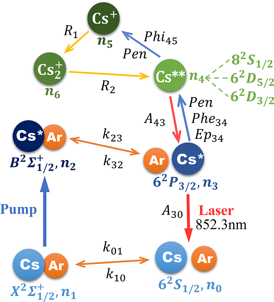
Figure 2 Diagram of energy states in high-power XPCsL system.
The rates of laser emission  ${L}_{30}$ and pump absorption ${P}_{12}$ are formulated as
 $$\begin{align}{L}_{30}\left(x,y,z\right)&=\left[{n}_3\left(x,y,z\right)-2{n}_0\left(x,y,z\right)\right]{\sigma}_{D1}\notag\\&\quad{}\cdot \frac{f_l\left(x,y,z\right)\left[{P}_l^{+}\left(x,y,z\right)+{P}_l^{-}\left(x,y,z\right)\right]}{h{\nu}_l},\end{align}$$
 $$\begin{align}{P}_{12}\left(x,y,z\right)&=\left[{n}_1\left(x,y,z\right)-{n}_2\left(x,y,z\right)\right]\notag\\&\quad{}\cdot \int \frac{\sigma_{D2}\left(\nu \right){f}_p\left(x,y,z\right){P}_p\left(x,y,z,\nu \right)}{h{\nu}_p} \mathrm{d}\nu,\end{align}$$
where  ${\sigma}_{D2}$ is the spectrally resolved atomic absorption cross-section and ${\sigma}_{D1}$ is the stimulated emission cross-section.
The pump beam at  $z=0$ is described as
 $$\begin{align}{P}_p\left(x,y,0,\nu \right)={P}_{p,0}\frac{2}{\nu_p}\sqrt{\frac{\ln 2}{\pi }}\exp \left[-4\ln 2\frac{{\left(\nu -{\nu}_p\right)}^2}{\Delta {\nu_p}^2}\right],\end{align}$$
where  ${\nu}_p$ and $\Delta {\nu}_p$ are the central frequency and the full width at half maximum (FWHM) of the pump beam, respectively, ${P}_{p,0}$ denotes the pumping power in total, and ${f}_p$ and ${f}_l$ depict the light intensity distribution of the pump and laser beam at (x, y, z), written as
 $$\begin{align}{f}_{p,l}\left(x,y,z\right)=\frac{\sqrt{2}}{\pi {w}_{p,l}{(z)}^2}\exp \left\{-\sqrt{2}\left[\frac{x^2+{y}^2}{w_{p,l}{(z)}^2}\right]\right\},\end{align}$$
where  ${w}_p(z)$ and ${w}_l(z)$ are the radii of pump and laser beam at z,
 $$\begin{align}{w}_{p,l}(z)={w}_{0,p,l}\sqrt{{\left[\frac{\left(z-{z}_{0,p,l}\right){\lambda}_{p,l}}{\pi {w}_{0,p,l}}\right]}^2+1},\end{align}$$
where  ${z}_{0,p,l}$ are the z-coordinates of the pump and laser beam waists ( ${w}_{0,p,l}$).
The other parameters involved in the rate equations are listed in Table 1.
Table 1 Kinetic processes in the XPAL system.

2.2 Solution for laser power
The propagations of laser and pump lights along the z-axis are described by the following iterative equations:
 $$\begin{align}&{P}_p\left(x,y,z+\Delta z\right)={P}_p\left(x,y,z\right)\cdot \sum \limits_S{f}_p\left(x,y,z\right)\notag\\&\quad{}\cdot\exp \left\{-\left[{n}_1\left(x,y,z\right)-{n}_2\right(x,y,z\left)\right]{\sigma}_{D2}\left(\nu \right)\Delta z\right\}\Delta x\Delta y,\\\end{align}$$
 $$\begin{align}&{P}_l^{\pm}\left(x,y,z+\Delta z\right)={P}_l^{\pm}\left(x,y,z\right)\cdot \sum \limits_S{f}_l\left(x,y,z\right)\notag\\&\quad{}\cdot\exp \left\{\pm \left[{n}_3\left(x,y,z\right)-2{n}_0\right(x,y,z\left)\right]{\sigma}_{D1}\Delta z\right\}\Delta x\Delta y,\end{align}$$
where S is the cross-section of the cell.
The initial boundary conditions of  ${P_l}^{+}$ and ${P_l}^{-}$ at z = 0 are given by
 $$\begin{align}{P}_l^{-}(0)&=\frac{P_l}{{T}_l\left(1-{R}_{\mathrm{oc}}\right)},\end{align}$$
 $$\begin{align}{P}_l^{+}(0)&=\frac{P_l{T}_l{R}_{\mathrm{oc}}}{1-{R}_{\mathrm{oc}}}.\end{align}$$
 To calculate the output power of the laser, we first assume a laser output power value and then substitute it into the initial equation at z = 0 for iterative operation. If the boundary equation  ${P_l}^{-}(l)={P_l}^{+}(l){T_l}^2{T_s}^2{R}_p$ at $z=L$ is satisfied, the correct output laser power is obtained, where ${R}_{\mathrm{oc}}$ and ${R}_p$ are the reflectivity of the OC and the back reflector, ${T}_l$ is the single-pass cell window transmission, and ${T}_s$ is the intra-cavity single-pass loss.
2.3 Calculation of temperature distribution
The heat generated by multiple transitions in each volume element is given by
 $$\begin{align}\varOmega \left(x,y,z\right)&=\Delta x\Delta y\Delta z\{[{k}_{01}{n}_0\left(x,y,z\right)\left[\mathrm{Ar}\right]-{k}_{10}{n}_1\left(x,y,z\right)]\notag\\&\quad{}\cdot\Delta {E}_{10}+[-{k}_{32}{n}_3\left(x,y,z\right)\left[\mathrm{Ar}\right]+{k}_{23}{n}_2\left(x,y,z\right)]\notag\\&\quad{}\cdot\Delta {E}_{23}+{R}_2\left(x,y,z\right){E}_{\mathrm{io}}\},\end{align}$$
where  $\Delta E$ denotes the energy gap of the corresponding levels and ${E}_{\mathrm{io}}$ is the ionization energy.
2.3.1. Temperature distribution without medium flow
The heat dissipation in the cell is mainly attributed to heat conduction when u = 0, which can be expressed as
 $$\begin{align}{H}_c\left(x,y,z\right)=2\pi \Delta z\frac{k_e\left[T\left(x,y,z\right)-{T}_w\right]}{\ln \left(R/\sqrt{x^2+{y}^2}\right)},\end{align}$$
where  ${k}_e$ is the effective thermal conductivity[Reference Barmashenko and Rosenwaks28] and R is the radius of the cell. Here $T\left(x,y,z\right)$ can be obtained by the heat balance $\varOmega \left(x,y,z\right)={H}_c\left(x,y,z\right)$.
2.3.2. Temperature distribution with medium flow
The heat removed in each volume by flowed gases with different direction can be calculated by
 $$\begin{align}{F}_L\left(x,y,z\right)&=\left\{\!\!\!\displaystyle\begin{array}{l}\frac{u\Delta x\Delta y{n}_t\left(x,y,z\right)}{N_A}{\int}_{T_w}^{T\left(x,y,z\right)}{C}_p\left(T^{\prime}\right)\;\mathrm{d}T^{\prime },\kern1.44em z=0,\\{}\frac{u\Delta x\Delta y{n}_t\left(x,y,z\right)}{N_A}{\int}_{T\left(x,y,z-\Delta z\right)}^{T\left(x,y,z\right)}{C}_p\left(T^{\prime}\right)\;\mathrm{d}T^{\prime },\kern0.84em z>0,\end{array}\right.\end{align}$$
 $$\begin{align}{F}_T\left(x,y,z\right)&=\left\{\!\!\!\displaystyle\begin{array}{l}\frac{u\Delta z\Delta y{n}_t\left(x,y,z\right)}{N_A}{\int}_{T_w}^{T\left(x,y,z\right)}{C}_p\left(T^{\prime}\right)\;\mathrm{d}T^{\prime },\kern2.04em x=0,\\{}\frac{u\Delta z\Delta y{n}_t\left(x,y,z\right)}{N_A}{\int}_{T\left(x-\Delta x,y,z\right)}^{T\left(x,y,z\right)}{C}_p\left(T^{\prime}\right)\;\mathrm{d}T^{\prime },\kern1.44em x>0,\end{array}\right.\end{align}$$
where  ${F}_L\left(x,y,z\right)$ and ${F}_T\left(x,y,z\right)$ denote the heat removed by longitudinal flow and transverse flow, respectively, u and ${n}_t$ are the velocity and number density of the total mixed gases, and ${C}_P(T)$ is the average molar heat capacity of the mixed gases.
On the other hand, the heat transferred by heat conduction in each volume element can be written as
 $$\begin{align}\varPhi \left(x,y,z\right)&=K\left(x,y,z\right) Nu\left(x,y,z\right)\notag\\&\quad{}\cdot \Big\{\frac{\Delta x\Delta y}{\Delta z}\left\{\left[T\left(x,y,z+\Delta z\right)-T\left(x,y,z\right)\right]\right.\notag\\&\qquad\left.-\left[T\left(x,y,z\right)-T\left(x,y,z-\Delta z\right)\right]\right\}\notag\\&\quad{}+\frac{\Delta y\Delta z}{\Delta x}\left\{\left[T\left(x+\Delta x,y,z\right)-T\left(x,y,z\right)\right]\right.\notag\\&\qquad\left.-\left[T\left(x,y,z\right)-T\left(x-\Delta x,y,z\right)\right]\right\}\notag\\&\quad{}+\frac{\Delta z\Delta x}{\Delta y}\left\{\left[T\left(x,y+\Delta y,z\right)-T\left(x,y,z\right)\right]\right.\notag\\&\qquad\left.-\left[T\left(x,y,z\right)-T\left(x,y-\Delta y,z\right)\right]\right\}\Big\},\end{align}$$
where K and Nu are the thermal conductivity and Nusselt number[Reference Barmashenko and Rosenwaks28], respectively.
Then the temperature  $T\left(x,y,z\right)$ in each volume element can be obtained from the following balance equation:
 $$\begin{align}\varOmega \left(x,y,z\right)={F}_{L,T}\left(x,y,z\right)+\varPhi \left(x,y,z\right).\end{align}$$
3 Results and discussion
3.1 Comparison with experimental result
Figure 3 is the comparison of slope efficiency between experiment[Reference Endo, Nagai and Wani19] and simulation results with the parameters listed in Table 2. A laser pulse train with FWHM of 40 ns is used in experiment, generating a  $\sim {10}^4$ W of peak power for optical pump. Good agreement between simulation and experiments can be seen at the slope efficiency.

Figure 3 Comparison of slope efficiency between experiment[Reference Endo, Nagai and Wani19] and simulation results.
Table 2 Parameters of experiment and simulation.

3.2 Three-dimensional distribution of temperature
The temperature distribution in the gain medium can highly influence the output performance especially on the beam quality. Figure 4 presents the three-dimensional distribution of temperature in the cell under conditions of longitudinal and transverse gas flow, where the velocity of flow and wall temperature are both set at 50 m/s and 473 K, respectively. As shown in Figure 4(a), the temperature distribution is circularly distributed and outward diffuses whereas it is elliptically outwardly distributed in Figure 4(b). The maximum temperatures in Figures 4(a) and 4(b) are 831.4 and 495.9 K, indicating an advantage that transverse flow can take in temperature control. On the other hand, comparing Figures 4(a) with 4(b), one can note that the maximum point of temperature in the x–y plane is shifted from (0, 0) to (0.7, 0) when the cooling flow is changed from longitudinal to transverse. Therefore, though the longitudinal gas flow can effectively reduce the temperature overall, it also creates a new temperature gradient in the z-axis direction, whereas the transverse flow avoids this problem by moving the majority of heat away from the optical axis. In general, the transverse gas flow can more effectively control the paraxial temperature, so that improving the operating environment of laser system.

Figure 4 Three-dimensional temperature distribution under different flow directions. The velocity of flow and wall temperature in (a) and (b) are 50 m/s and 473 K.
Figure 5 shows the more detailed distribution of temperature and  ${N}_{\mathrm{Cs}}$ on the x–z plane at y = 0 in Figure 4. The gas flow is longitudinal in Figures 4(a) and 4(c) and transverse in Figures 4(b) and 4(d). As ${N}_{\mathrm{Cs}}\left(x,y,z\right)={n}_{\mathrm{Cs}}{T}_w\left(x,y,z\right)/T\left(x,y,z\right)$, it can be seen from the comparison between the upper and lower graphs that the particle number densities are relatively lower in aera with high temperatures, resulting in a decay of output performance. The lowest ${N}_{\mathrm{Cs}}$ in Figures 5(c) and 5(d) are $1.0469\times 1{0}^{21}\;{\mathrm{m}}^{-3}$ and $1.7313\times 1{0}^{21}\;{\mathrm{m}}^{-3}$, respectively. Moreover, the particle number density around the optical axis in Figure 5(d) is less affected. As a result, with $u=50\;\mathrm{m/s}$, ${T}_w=473\;\mathrm{K}$, and ${I}_P=4.5\times 1{0}^6\;\mathrm{W}/\mathrm{cm}^2$, the optical-to-optical efficiency is 2.05% under transverse gas flow while that is 1.23% under longitudinal gas flow, proving the former can improve the laser output performance of an XPCsL.

Figure 5 (a), (b) The temperature distribution in the x–y plane at y = 0 in Figures 4(a) and 4(b). (c), (d) The distribution of  ${N}_{\mathrm{Cs}}$ in the x–y plane at y = 0 in Figures 4(a) and 4(b).
3.3 Influence of flow on optical-to-optical efficiency
In Section 3.2, we confirm that the temperature distribution in the gain medium can affect the output performance of the laser by changing distribution of the number density of Cs particles. Therefore, in this section, we take the maximum temperature as an indicator to characterize the temperature gradient in the cell, and further study the influences of pump intensity, wall temperature, and gas flows with different directions and velocities on the optical-to-optical efficiency. The parameters used in the simulation are listed in Table 3.
Table 3 Parameters used in the simulation.

Figure 6 depicts the optical-to-optical efficiency and maximum temperature as a function of flow velocity with different pump intensity at Tw = 473 K. One can see from Figure 6 that severe heat accumulation will occur in the gain medium during the operation without gas flow, which greatly limits the output performance of laser. The optical-to-optical efficiency in Figures 6(a) and 6(b) increases with the rise of flow velocity and pump intensity, and then tends to be saturated, while the maximum temperature in Figures 6(c) and 6(d) is the opposite. In the case of longitudinal gas flow, in the range of 0 to ~50 m/s, the maximum temperature and optical-to-optical efficiency are more sensitive to the change of fluid velocity, whereas that range in Figures 6(b) and 6(d) is 0 to ~10 m/s. In particular, in Figure 6(d), the effect of the fluid velocity on the temperature gradient in the gain medium is relatively small after crossing 20 m/s. Furthermore, the laser output tends to be saturated with a transverse gas flow of ~50 m/s, whereas ~250 m/s of longitudinal gas flow is needed in the same situation.

Figure 6 Optical-to-optical efficiency and maximum temperature as a function of flow velocity with different pump intensity at Tw = 473 K.
On the other hand, compared with Figures 6(a) and 6(c), the slopes of the curves in Figures 6(b) and 6(d) are larger, respectively, indicating that the transverse gas flows have a better heat dissipation efficiency. In addition, under the same conditions, the maximum temperature in the cell is always lower with transverse gas flow, resulting in a higher laser output.
The relationship between optical-to-optical efficiency and flow velocity with different wall temperature at a pump intensity of 5 × 10¹⁰ W/m2 is plotted in Figure 7, in which the conclusions obtained in Figure 6 can also be confirmed. In addition, the maximum temperature in Figure 7 rises and is higher than that in Figure 6 when u = 0 as the wall temperature increases. In other words, a higher wall temperature is more likely to generate a larger heat load in the gain medium. In the case of u > 0, the slope of curve representing the maximum temperature decreases significantly after the fluid velocity in Figures 7(c) and 7(d) reaches ~100 m/s and ~20 m/s, respectively. Comparing Figures 7(a) and 7(b) with Figures 6(a) and 6(b), it can be concluded that the wall temperature has a greater contribution to the improvement of optical-to-optical efficiency than the pump intensity. At the same time, a higher wall temperature means a higher flow velocity is required to reach the saturation value of the laser output, which is shown in Figures 7(a) and 7(b): with wall temperature higher than 503 K, longitudinal gas flow of quasi-sonic level and transverse gas flow greater than 50 m/s may be required to alleviate the thermal effect in the cell, maximizing the laser output.

Figure 7 Optical-to-optical efficiency and maximum temperature as a function of flow velocity with different wall temperature at pump intensity of 5 × 10¹⁰ W/m2.
4 Summary
In this paper, considering the kinetics, heat conduction, and fluid dynamics processes in the gain medium, we established a comprehensive three-dimensional physical model to simulate and analyze the laser output performance and temperature distribution in an XPCsL with longitudinal and transverse gas flow. The slope efficiency of laser calculated by the model is consistent with the experimental results. The three-dimensional distributions of temperature and number density of Cs particles in the cell with different directions of gas flow are simulated and depicted, demonstrating that the transverse gas flow can more effectively and uniformly alleviate the heat accumulation on the optical axis of pump light and laser, resulting in a higher particle number density of Cs in the cell. Furthermore, influences of pump intensity, wall temperature, and fluid velocity with different directions on maximum temperature in the cell and optical-to-optical efficiency are presented and analyzed in detail. The results indicate that the optical-to-optical efficiency increases with the pump intensity, wall temperature, and flow velocity. Increasing the wall temperature can better improve the potential of laser output than rising the pump intensity. Meanwhile, it will also cause a more significant heat accumulation in the gain medium, where higher-speed gas flow is required to alleviate it. On the other hand, compared with the longitudinal gas flow, the transverse gas flow with a lower velocity can more effectively remove the generated heat accumulation and reduce the temperature gradient in the cell to enhance the laser output. This work is of great help in revealing the kinetic and fluid dynamic mechanism and output characteristics in an XPCsL and promoting the realization of a high-efficiency fluid XPCsL.
Acknowledgement
This work was supported by the Aerospace Science and Technology Fund (No. KM20170269) and the National Natural Science Foundation of China (No. 11874322).


 Open access