


Introduction
With a growing global population to feed, increasing pressure is being placed on agricultural land to be more productive. Despite a steady increase in the global hectarage of arable land since the early 1960s, a sharp decline in the arable land per person has occurred over the same period (FAO 2018). This decline requires increased productivity of arable land. To raise land productivity, negative factors impacting yields must be minimized to meet the population demands for food. A significant contributor to crop yield loss is competition with weeds. Weeds can reduce yield in agronomic crops that contribute to the world food and fiber supply: 79% in soybean [Glycine max (L.) Merr.] (Bensch et al. Reference Bensch, Horak and Peterson2003), 91% in corn (Zea mays L.) (Massinga et al. Reference Massinga, Currie and Trooien2003), 90% in cotton (Gossypium hirsutum L.) (Rowland et al. Reference Rowland, Murray and Verhalen1999), and 29% in sorghum [Sorghum bicolor (L.) Moench] (Cramer and Burnside Reference Cramer and Burnside1982).
With the introduction of herbicide-resistant crops and the lack of rotation of herbicide chemistries, the agricultural ecosystem in production fields is changing due to increasing anthropogenic selection pressures on weed populations (Clements and Jones Reference Clements and Jones2021; Owen Reference Owen2008). This pressure over time has resulted in the selection of weed biotypes that are resistant to herbicides. Globally there are more than 515 species with resistance to at least one herbicidal mode of action (Heap Reference Heap2021). Some weed species have developed resistance to multiple herbicidal modes of action, making them difficult to control and allowing increased weed competition with crops. With resistance on the rise, weeds are often more difficult to control, and growers need to be able to monitor fields, identify weed species and densities, and determine the fluctuation of these weed populations between years. Collecting the aforementioned data on fields will allow growers to implement appropriately timed weed control measures and minimize crop loss due to weed interference. Crop losses associated with weed interference are estimated at $17 billion for soybean and $27 billion for corn, roughly 50% of the yield for each of these crops in the United States and Canada (Soltani et al. Reference Soltani, Dille, Burke, Everman, Vangessel, Davis and Sikkema2016, Reference Soltani, Dille, Burke, Everman, Vangessel, Davis and Sikkema2017). Recent surveys have indicated that Palmer amaranth (Amaranthus palmeri S. Watson) was in the top three most troublesome weeds in soybean, with large crabgrass [Digitaria sanguinalis (L.) Scop.] being a common weed throughout several other broadleaf cropping systems (Van Wychen Reference Van Wychen2019). Amaranthus palmeri is an erect, multibranched annual weed growing up to 2-m tall, producing greater biomass, and leaf area than other Amaranthus species (Bryson and DeFelice Reference Bryson and DeFelice2009; Horak and Loughlin Reference Horak and Loughlin2000). Digitaria sanguinalis is a prostrate to spreading summer annual with a height of 0.7 m (Bryson and DeFelice Reference Bryson and DeFelice2009; Holm et al. Reference Holm, Plunkett, Pancho and Herberger1991). Both species have high levels of fecundity and competition in cropping systems (Basinger et al. Reference Basinger, Jennings, Monks, Jordan, Everman, Hestir, Bertucci and Brownie2019; Norsworthy et al. Reference Norsworthy, Schrage, Barber and Schwartz2016; Peters and Dunn Reference Peters and Dunn1971). Concerns from the public about weed resistance, environmental impacts of pesticides, and possible restrictions on herbicide use may force new management strategies for weeds.
To minimize direct or indirect crop loss to weeds, weed management is critical. One approach to weed management is the use of site-specific weed management. Site-specific weed management is designed to control weeds only where they are present and to reduce the environmental impacts of herbicide applications and tillage. Site-specific management can reduce herbicide inputs, soil compaction, energy consumption, and off-target herbicide application (Brown and Noble Reference Brown and Noble2005; Coleman et al. Reference Coleman, Stead, Rigter, Xu, Johnson, Brooker, Sukkarieh and Walsh2019; Fernandez-Quintanilla et al. Reference Fernandez-Quintanilla, Pena, Andujar, Dorado, Ribeiro and Lopez-Granados2018). Site-specific management requires accurate scouting of fields to determine whether weed management is needed or to accurately detect and identify weeds (Hunter et al. Reference Hunter, Gannon, Richardson, Yelverton and Leon2019; Li et al Reference Li, Al-Sarayreh, Irie, Hackell, Bourdot, Reis and Ghamkhar2021). In agronomic crops, weed management must take place early in the season to minimize the interference weeds have in the crops. To do so, scouting for weeds must be done at targeted timings to determine the appropriate time for the implementation of weed control. Recommendations resulting from a scouting exercise are frequently tied to the quality of the scouting data, and accurate scouting can be time-consuming. Remote sensing may provide a solution for accurate and timely scouting of agricultural fields. Remote sensing has been utilized in agriculture to predict yield and biomass (Chen et al. Reference Chen, Shang Zhao and Tao2018; Yue et al. Reference Yue, Feng, Li, Shou and Xu2021), determine crop nutrient or water stress (Basso et al. Reference Basso, Fiorentino, Cammarano and Schulthess2016; Bellvert et al. Reference Bellvert, Zarco-Tejada, Girona and Fereres2014; Mahajan et al. Reference Mahajan, Pandy, Sahoo, Gupta, Datta and Kumar2017) and crop–weed competition (Ronay et al. Reference Ronay, Ephrath, Eizenberg, Blumberg and Maman2021), and detect the presence of insects or plant disease (Abudulridha et al. Reference Abdulridha, Ampatzidis, Roberts and Kakarla2020; Franke and Menz Reference Franke and Menz2007; Rhodes et al. Reference Rhodes, Bennie, Spalding, ffrench-Constant and Maclean2022). Remote sensing for weed detection has been attempted since the early 1980s (Menges et al. Reference Menges, Nixon and Richardson1985; Richardson et al. Reference Richardson, Menges and Nixon1985). These attempts at weed detection, along with later attempts (Brown et al. Reference Brown, Steckler and Anderson1994; Everitt et al. Reference Everitt, Pettit and Alaniz1987, Reference Everitt, Escobar, Alaniz, Villarreal and Davis1992; Medlin et al. Reference Medlin, Shaw, Gerard and LaMastus2000; Yang and Everitt Reference Yang and Everitt2010), were successful in discriminating weeds but unable to connect discrimination to management decisions.
Research focused on remote sensing of weeds and invasive species has used satellite data or data collected using aerial sensors (Hunt et al. Reference Hunt, Daughtry, Kim and Parker-Williams2007; Menges et al. Reference Menges, Nixon and Richardson1985). These methods often lack the spatial and temporal resolution to detect weeds intermixed with crops. Some of these limitations have been overcome through the use of unmanned aerial vehicles (UAVs); however, there are still limitations to this technology (Huang et al. Reference Huang, Reddy, Fletcher and Pennington2018). Additionally, many studies have been conducted using spectrally limited sensors and may only contain wavelengths in the visible (VIS) or shortwave portions of the near-infrared (NIR) spectrum. The use of hyperspectral remote sensing has allowed for discrimination of weed species (Gray et al. Reference Gray, Shaw and Bruce2009) and detection of herbicide drift (Huang et al. Reference Huang, Yuan, Reddy and Zhang2016; Suarez et al. Reference Suarez, Apan and Werth2017) in agricultural settings. Hyperspectral data provide greater spectral resolution and could allow for the detection of differences between crop and weed species while also detecting biophysical differences. Research utilizing hyperspectral data that account for weed density and crop/weed phenology as a means of weed detection is limited. Studies examining reflectance spectra often are conducted in only a single year (Koger et al. Reference Koger, Shaw, Reddy and Bruce2004b) or have limited temporal data-collection dates (Goel et al. Reference Goel, Prasher, Landry, Patel, Bonnell, Viau and Miller2003; Hunt et al. Reference Hunt, Daughtry, Kim and Parker-Williams2007).
Recent approaches have begun to bridge the gaps between data collection, weed discrimination, and management decisions through the aggregation of technologies. The implementation of UAVs and other technologies for the discrimination of weeds must rely on in situ data collection to ground-truth UAV data (Huang et al Reference Huang, Yuan, Reddy and Zhang2016; Shafian et al. Reference Shafian, Rajan, Schnell, Bagavathiannan and Valasek2018; Suarez et al Reference Suarez, Apan and Werth2017) and elucidate relationships not detected by sensors on a UAV. The integration of the information from these technologies not only improves the discrimination of weeds from crops but allows for the implementation of real-time control measures (Hu et al. Reference Hu, Coleman, Zeng, Wang and Walsh2020; Hunter et al. Reference Hunter, Gannon, Richardson, Yelverton and Leon2019). Despite the best efforts to integrate these technologies, research using in situ remote sensing is needed to continue to improve the accuracy of current and future hyperspectral UAV and ground-based weed management systems. These systems could be greatly improved by identifying novel reflectance regions that could be leveraged for species discrimination and detection. Thus, the objectives of this study are to determine (1) whether weed species can be differentiated in situ, (2) the effect of soybean and weed phenology on differentiation, (3) the effect of weed species and density on hyperspectral reflectance, and (4) the effect of crop presence on weed detection and density differentiation.
Materials and Methods
Field studies were conducted on ‘AG6536’ soybean in 2016 and 2017 at the Horticultural Crops Research Station near Clinton, NC (35.0242°N, 78.2828°W). The studies were conducted on a Norfolk loamy sand (fine-loamy, kaolinitic, thermic Typic Kandiudults) with 0.31% humic matter and pH 5.9 and an Orangeburg loamy sand (fine-loamy, kaolinitic, thermic Typic Kandiudults) with 0.47% humic matter and pH 5.9 in 2016 and 2017, respectively.
Experimental Design and Treatments
‘AG6536’ soybean was planted at a seeding rate of 321,000 seeds ha−2 (10-cm in-row spacing) using a four-row vacuum planter on June 9, 2016, and June 12, 2017. Treatments were combinations of crop presence or absence, weed species (A. palmeri or D. sanguinalis), and weed density (1, 2, 4, 8 and 1, 2, 4, and 16 plants m−2, respectively) arranged in a randomized complete block design with three replications. Plots consisted of 4 rows, each 30-cm wide by 5-m long. The day following crop planting, designated plots were seeded by hand with each weed species. In plots designated as no crop, soybean was pulled upon emergence. Amaranthus palmeri at approximately 8-cm tall and D. sanguinalis at two expanded leaves were thinned to 1, 2, 4, 8 and 1, 2, 4, and 16 plants m−2, respectively, then maintained weekly using hand removal. Additionally, a plot containing no weeds served as a weed-free check plot, and a plot containing no crops and no weeds was utilized as a bare-ground treatment.
Data Collection
Spectral data were collected across five dates in 2016 and six dates in 2017 to determine the effect of phenology on spectral variability and for detection of weed species and density. Spectral measurements were collected using a spectrometer (PSM-2500, Spectral Evolution, 1 Canal Street, Lawrence, MA 01840) with fiber optic capable of a 44-rad field of view (0.44 m−2 ground field of view for each reading), between 1000 and 1400 hours, in full sunlight. Spectra were collected and graphed at the time of collection using data-acquisition software (Darwin SP, Spectral Evolution). The spectrometer has a spectral resolution of 3.5 nm at 700 nm, 22 nm at 1,500 nm, and 22 nm at 2,100 nm. Data output is in 1-nm increments, resulting in 2,151 bands reported. To account for environmental and atmospheric variability during each data-collection date, the sensor was calibrated every 15 min using a white reflectance panel (Spectralon, Labsphere, 231 Shaker St, North Sutton, NH 03260). Spectrometer measurements were taken at nadir. A meter stick was placed at the apex of the average plant height in the plot to ensure that all measurements were taken 1 m over the plot canopy. Five measurements were taken for each plot to capture crop and weed variability across the plot area, including soil background, with a plot with no soybean and no weeds serving as a bare-ground plot for soil reference. The bare-ground plot served as a negative control to ensure that spectra from crops, weeds, mixed spectra of crops, and weeds were able to be differentiated from the soil. Crop and weed phenology and heights were determined based on methods by Meier (Reference Meier2018) at each spectral data collection.
Data Processing
Hyperspectral data for each plot and date were graphed using the ggplot2 package in R software (v. 3.4.2) (Wickham Reference Wickham2013). Visual quality control was performed for each graph, and data containing interference or noise as noted in field notes were removed. Reflectance spectra were then grouped by date, weed type, and the presence or absence of crop. Each subset of data was subjected to the Kruskal-Wallis test to determine overall groupwise differences at each of the 2,151 bands reported (Corder and Foreman Reference Corder and Foreman2009). Comparisons were made by wavelength band to determine species differentiation. To determine differences within each subset of data, differences at each reported band were tested using the Mann-Whitney U-test (Corder and Foreman Reference Corder and Foreman2009; Schmidt and Skidmore Reference Schmidt and Skidmore2003). The null hypothesis being tested states that median reflectance for each reported band is not different between weed species or density. Levels of significance were set at P ≤ 0.1 due to limits in sample size and to explore a range in which additional wavelengths may provide confidence in the differentiation of weed species and density. P-values are reported as a continuous variable for each wavelength, where P ≤ 0.1. In an agricultural setting like the one in which this study was conducted, outcomes of misidentification would result in mistaking a crop plant for weed or vice versa. If site-specific weed management is the goal, discrimination of weeds at a P ≤ 0.1 level would prove beneficial for use in a weed control program.
Results and Discussion
Differentiation of All Treatments
Throughout the rest of this paper, results for spectra will be discussed corresponding to the following spectral regions: visible (VIS = 350 to 700 nm), near-infrared (NIR = 700 to 1,300 nm), shortwave-infrared region 1 (SWIR1 =1,500 to 1,900 nm), and shortwave-infrared region 2 (SWIR2 = 1,900 to 2,500 nm). The shortwave-infrared spectral region was subdivided into SWIR1 and SWIR2 to provide more meaningful results given the large spectral range of the SWIR region.
Groupwise differentiation including all combinations of weed species, weed density, and crop presence or absence were compared with one another (Figures 1 and 2). Spectral reflectance was different across years and the varying crop and weed phenological time points at which the spectra were collected. Therefore, data are presented by year and weeks after planting (WAP). In 2016, differentiation between weed species, density, and crop presence was most prevalent across spectra at 5 WAP. The differentiation at this timing was when there was the greatest difference in vegetation cover between the plots containing soybean and the plots containing only weeds. Plots containing lower weed densities at this timing were more spectrally similar to the bare-ground plots. At this point in the season, weeds canopies were not large enough to fill the entirety of the plots as they did late season. For plots containing soybean or higher weed densities, spectra were more similar due to greater amounts of vegetation when compared with the bare-ground and lower weed density plots. This trend was similar in 2017 at 3, 4, and 5 WAP (Figure 2).
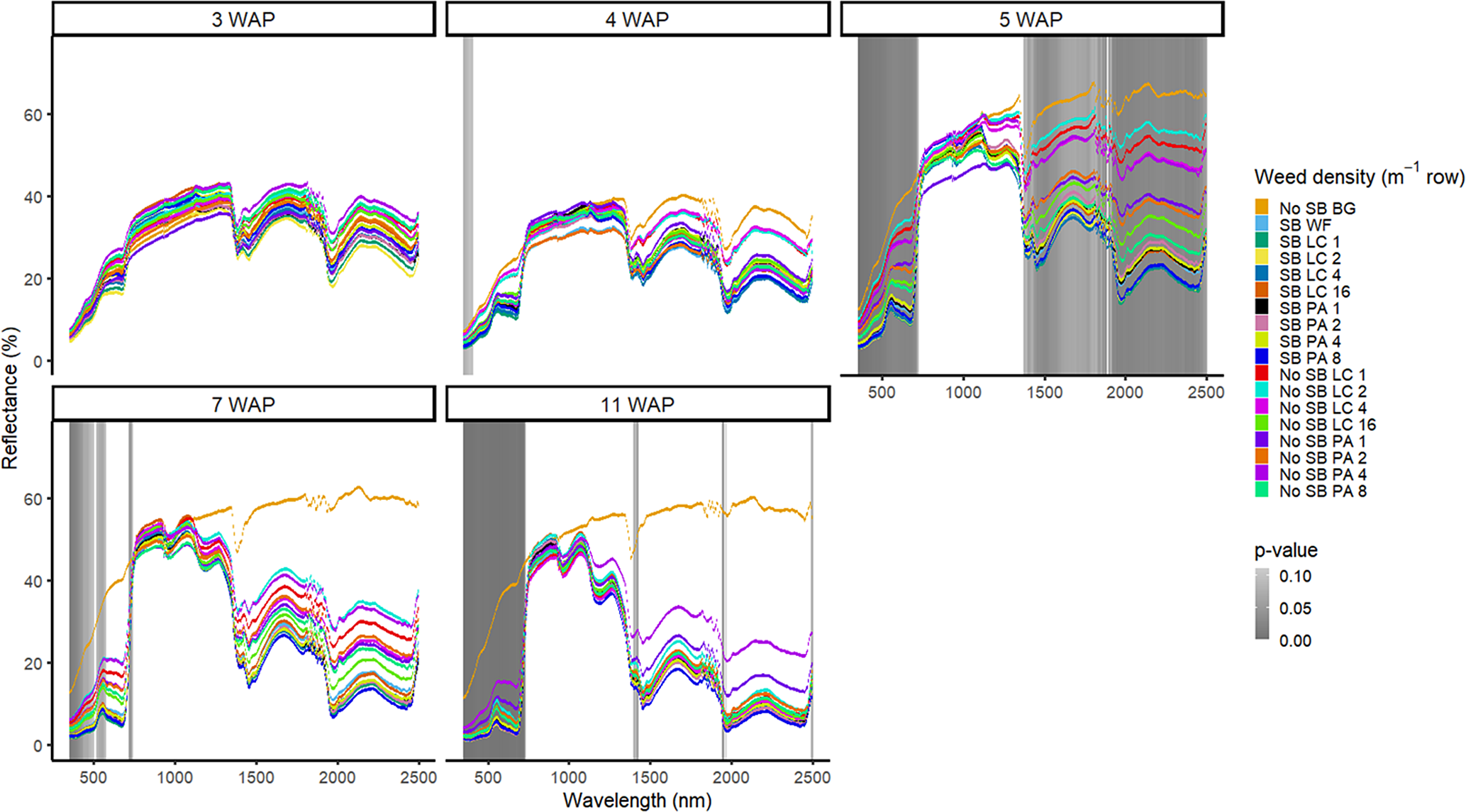
Figure 1. Spectral reflectance for all Amaranthus palmeri (PA) and Digitaria sanguinalis (LC) densities with (SB) and without soybean at the Horticultural Crops Research Station, Clinton, NC, 2016. Bare ground (No SB BG) and weed-free soybean (SB WF) were grouped by weeks after planting (WAP).
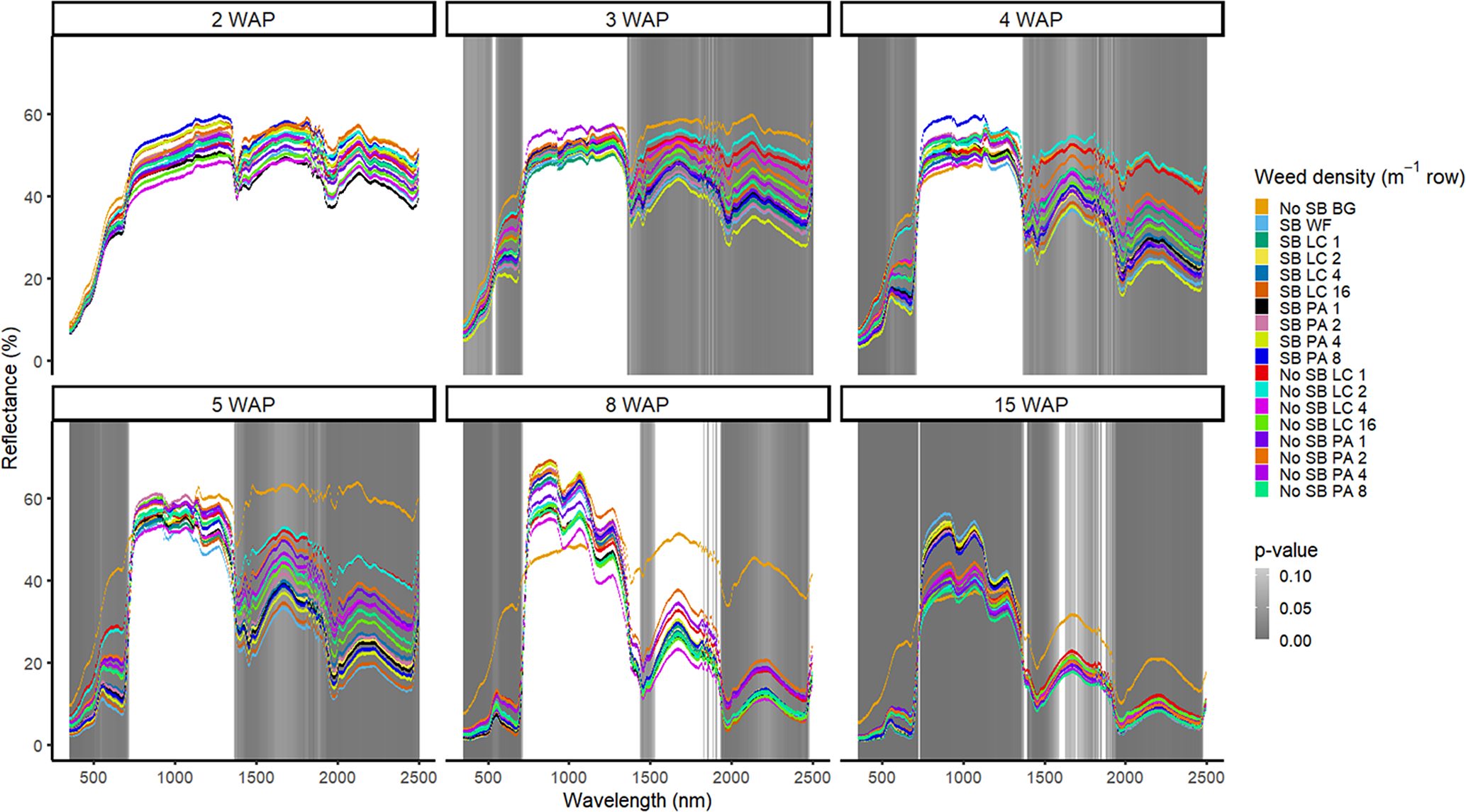
Figure 2. Spectral reflectance for all Amaranthus palmeri (PA) and Digitaria sanguinalis (LC) densities with (SB) and without soybean at the Horticultural Crops Research Station, Clinton, NC, 2017. Bare ground (No SB BG) and weed-free soybean (SB WF) were grouped by weeks after planting (WAP).
Other spectral differences in 2016 were seen at 4, 7, and 11 WAP and were confined to spectral reflectance and absorption magnitude differences in the VIS (Figure 1). This was due to the inclusion of the bare-ground treatment, for which differences were observed in spectral magnitude in the VIS and SWIR1 and SWIR2. In 2017, however, differences were seen across the VIS and both SWIR1 and SWIR2 from 3 WAP to 15 WAP. At 15 WAP, additional spectra of interest were noted in the NIR region (Figure 2). Early-season differentiation was not possible between weeds and bare ground at 2 and 3 WAP in 2016 and 3 WAP in 2017. At this time point, weeds are at an optimal stage for control using chemical or mechanical control measures due to their small size (<10 cm). During both years, there were differences in spectral magnitude that are associated with changes in the type (weed species vs. crop) and amount (weed density) of vegetation present. Furthermore, spectral reflectance curves were not constant between reading dates, as these curves change in magnitude and shape with changing plant phenology, crop presence, and weed species and density
Differentiation of Weed Species
In 2016, weed species could not be differentiated from one another regardless of species or weed density in the presence of soybean (Figure 3). Soybean reduced weed biomass (Basinger et al. Reference Basinger, Jennings, Monks, Jordan, Everman, Hestir, Bertucci and Brownie2019), which could have affected the ability to have spectral differences between both weed species and weed density. Similar results were seen without soybean present; only a few spectra in the blue range at 5 WAP showed differences between weed species (Figure 4). When compared with bare ground, all of the plots containing weeds at any density had greater absorbance in the blue region. The blue region of the spectrum is associated with greater amounts of chlorophyll a and chlorophyll b as well as β-carotene (Jensen Reference Jensen2006; Mahlein et al. Reference Mahlein, Hammersley, Oerke, Dhene, Goldbach and Grieve2015), which would not be present in a plot with no vegetation. In 2017, results showed differences between weed species with soybean in blue spectra at 4 WAP and in the VIS and SWIR2 at 15 WAP (Figure 5). Differences in SWIR2 could be related to leaf water content or caused by competition within and between species, as greater reflectance could be a result of lower relative water content (Carter Reference Carter1991). Without soybean present, differences between species were detected across more spectra in the VIS at 3 to 15 WAP and in the SWIR1 and SWIR2 at 8 to 15 WAP (Figure 6). These late-season differences in the SWIR regions are tied to differences between the bare-ground plots and weed species and density due to the increased presence of foliage.
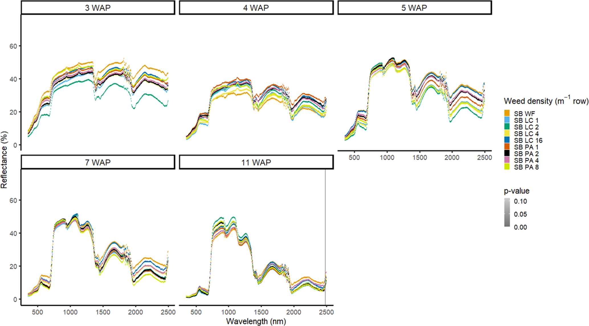
Figure 3. Spectral reflectance for all Amaranthus palmeri (PA) and Digitaria sanguinalis (LC) densities with soybean (SB) and a weed-free control (SB WF), grouped by weeks after planting (WAP), at the Horticultural Crops Research Station, Clinton, NC, 2016.

Figure 4. Spectral reflectance for all Amaranthus palmeri (PA) and Digitaria sanguinalis (LC) densities without soybean as a bare-ground control (No SB) grouped by weeks after planting (WAP), at the Horticultural Crops Research Station, Clinton, NC, 2016.

Figure 5. Spectral reflectance for all Amaranthus palmeri (PA) and Digitaria sanguinalis (LC) densities with soybean (SB) and a weed-free control (SB WF), grouped by weeks after planting (WAP), at the Horticultural Crops Research Station, Clinton, NC, 2017.
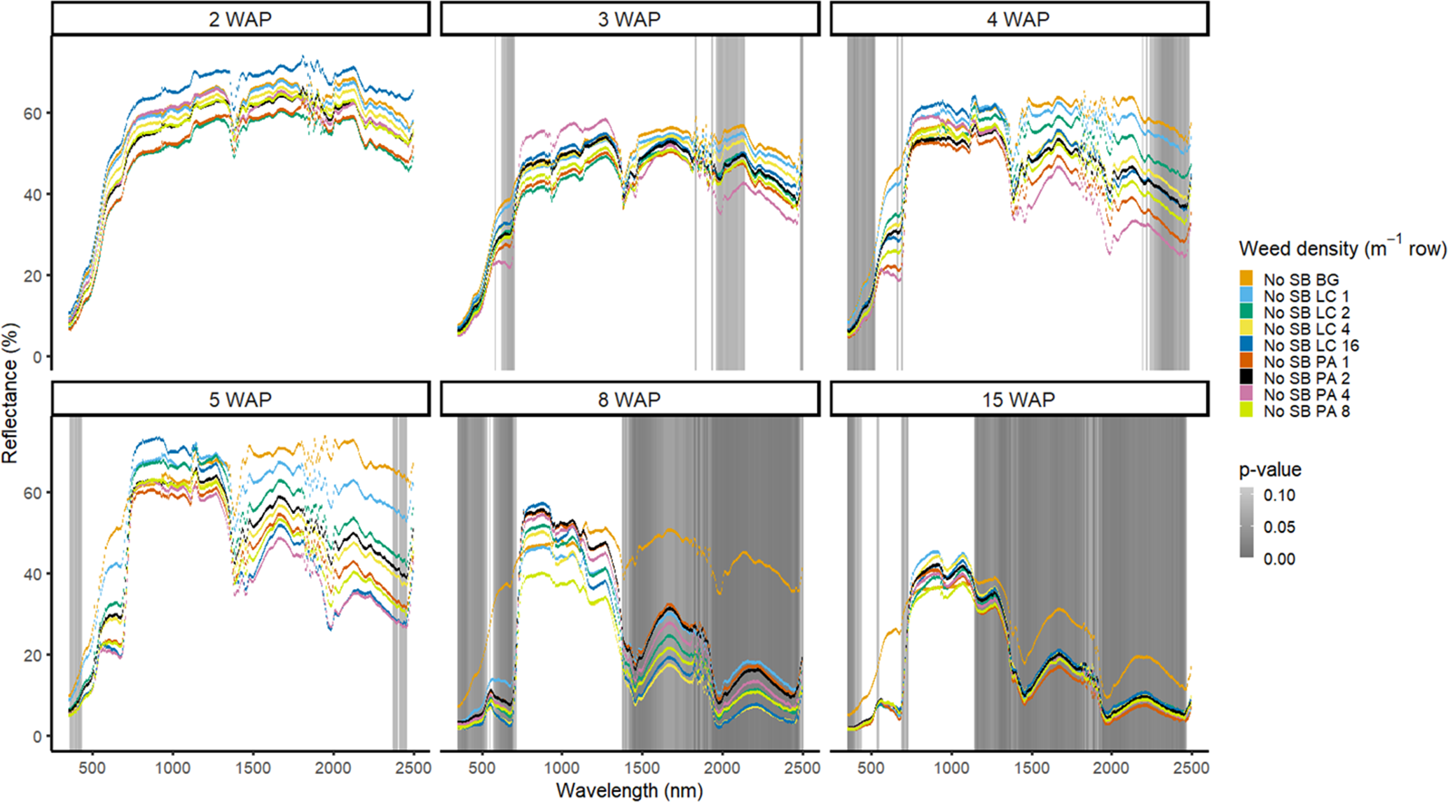
Figure 6. Spectral reflectance for all Amaranthus palmeri (PA) and Digitaria sanguinalis (LC) densities without soybean as a bare-ground control (No SB BG) grouped by weeks after planting (WAP), at the Horticultural Crops Research Station, Clinton, NC, 2017.
Results from this study show that spectral differentiation can occur between weed species and weed density. Successful discrimination of species in both agricultural and nonagricultural environments has previously been reported (Henry et al. Reference Henry, Shaw, Reddy, Bruce and Tamhankar2004; Koger et al. Reference Koger, Shaw, Reddy and Bruce2004a; Santos et al. Reference Santos, Hestir, Khanna and Ustin2011; Schmidt and Skidmore Reference Schmidt and Skidmore2003; Ustin et al. Reference Ustin, Gitelson, Schaepman, Asner, Gamon and Zarco-Tejada2009). However, the inconsistency of spectral differentiation across years and phenological time points complicates discrimination between species. Differences in environmental conditions from year to year may alter phenology, and spectra may not be uniform from year to year (Table 1). These differences may have caused spectral variation due to variable rainfall or other environmental changes between seasons.
Table 1. Mean monthly temperature, growing degree days (GDD), and precipitation for Clinton Horticultural Crops Research Station, Clinton, NC, from June to November for 2016 and 2017.

Weed species differentiation had limited spectra for weed species separation when in the presence of a crop and was not successful at low weed densities. The lack of differentiation at lower densities is likely due to the mixture of crop and limited weed species canopy. Weed biomass was lower when crops were present, and weed species at low densities often had limited canopy coverage over the crop, limiting their spectral contribution to the mixed spectra. (Basinger et al. Reference Basinger, Jennings, Monks, Jordan, Everman, Hestir, Bertucci and Brownie2019). Greater weed densities had higher biomass per square meter and contributed more to the mixed spectra. At the highest weed density, each species was more readily differentiated compared with the lower densities, due to increased weed canopy reflectance. Differentiation of weed species occurred later than would be acceptable for implementing chemical control of A. palmeri, but control options for D. sanguinalis would still be available.
Weed Density
Weeds with Soybean
The four densities of D. sanguinalis in the presence of soybean were not spectrally different from one another in 2016, except for only a few spectra in the NIR at 4 WAP (Figure 7). It would not be too late to control D. sanguinalis in soybean at 4 WAP (Van Acker et al. Reference Van Acker, Swanton and Weise1993). However, this difference at 4 WAP was not consistent between years and could not be relied on for making a management decision. In 2017, differences of D. sanguinalis with soybean were different at 4 WAP in the blue region of the VIS, and at 15 WAP throughout the VIS and in portions of the SWIR2 (Figure 8). The differences in blue regions at this time were likely tied to chlorophyll content at this time of the season (Jensen Reference Jensen2006; Mahlein et al Reference Mahlein, Hammersley, Oerke, Dhene, Goldbach and Grieve2015) However, the differences seen at 15 WAP were due to D. sanguinalis completing its life cycle and beginning to senesce and plant desiccation occurring while soybean was not physiologically mature. If D. sanguinalis was not detected, interference at the densities in this study could result in yield losses of up to 38% at 16 plants m−2 (Basinger et al. Reference Basinger, Jennings, Monks, Jordan, Everman, Hestir, Bertucci and Brownie2019).
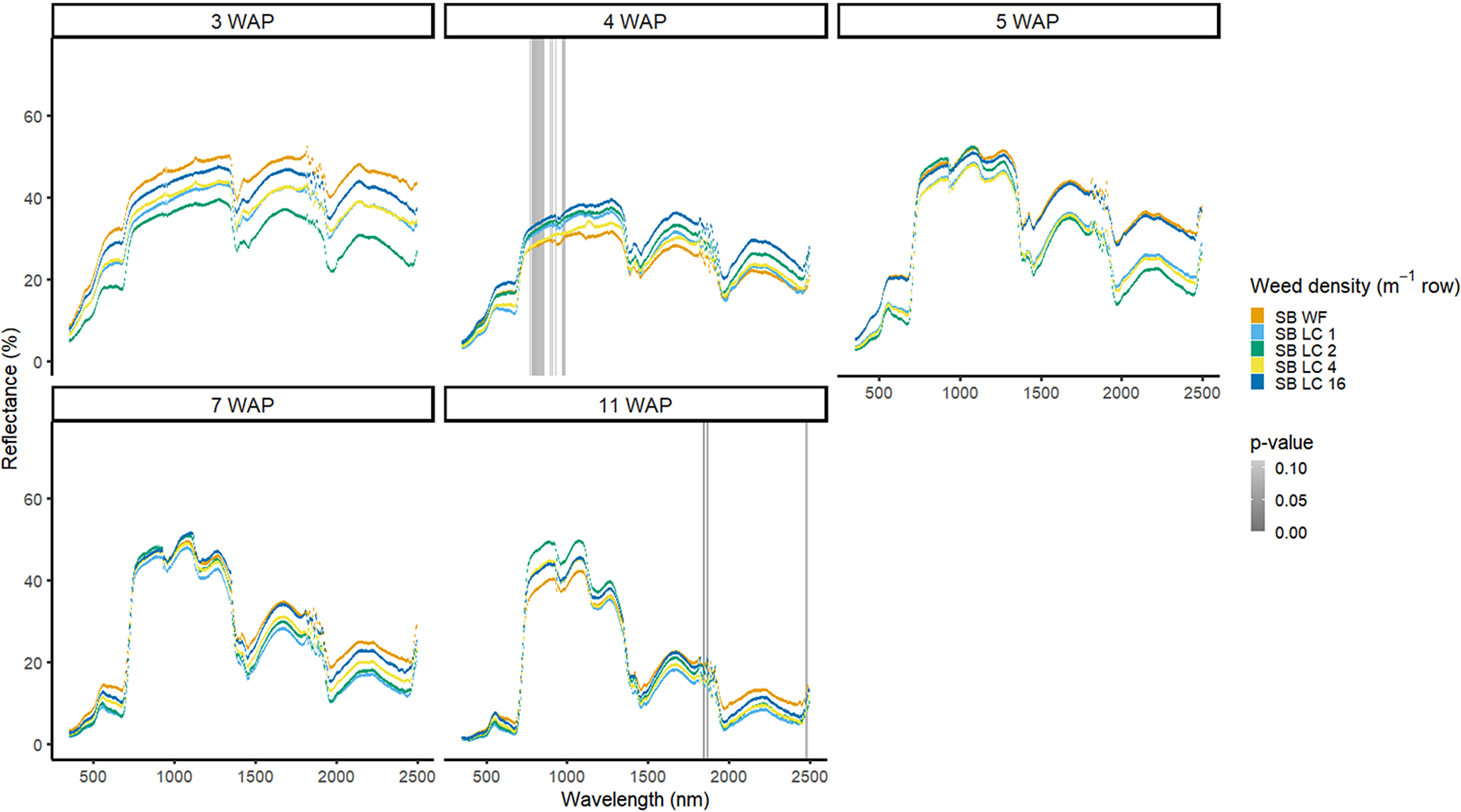
Figure 7. Spectral reflectance for all Digitaria sanguinalis (LC) densities with soybean (SB) and a weed-free control (SB WF), grouped by weeks after planting (WAP), at the Horticultural Crops Research Station, Clinton, NC, 2016.
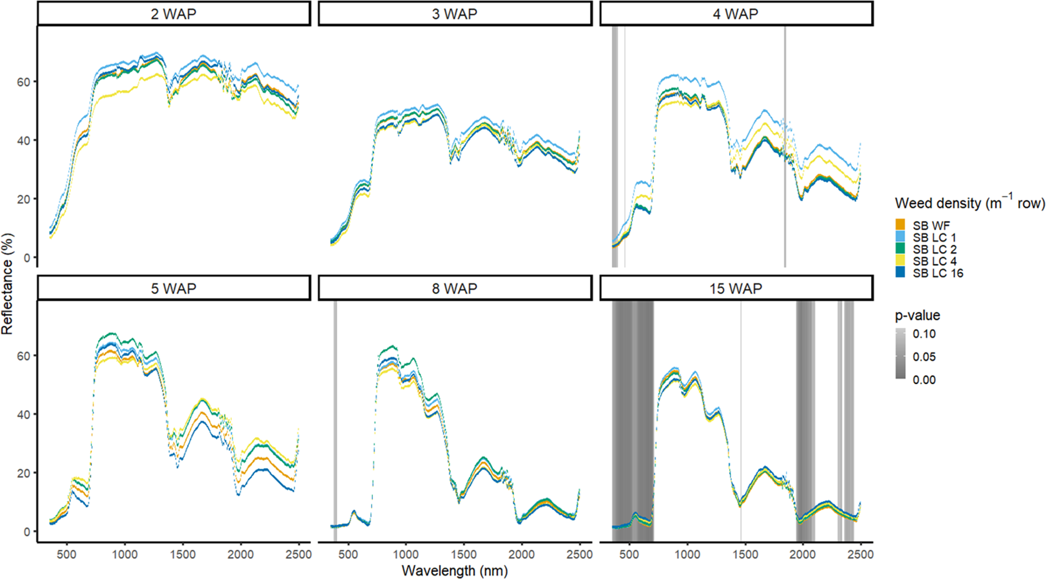
Figure 8. Spectral reflectance for all Digitaria sanguinalis (LC) densities with soybean (SB) and a weed-free control (SB WF), grouped by weeks after planting (WAP), at the Horticultural Crops Research Station, Clinton, NC, 2017.
Weed density with soybean present was more easily detected for A. palmeri than for D. sanguinalis. In 2016, in the presence of soybean, densities of A. palmeri were only different at limited spectra in the NIR at 4 WAP (Figure 9). All plots containing A. palmeri had greater reflectance in the NIR, which likely resulted from greater overall vegetation coverage at this point in the season (Table 2). In 2017, with soybean, spectral differences only occurred at 4 and 15 WAP in the VIS (Figure 10); differences at 15 WAP were likely due to the presence of reproductive structures in the plots containing A. palmeri and the beginning of senescence of the weeds in the plots. At 15 WAP, pairwise comparisons between the weed-free treatment and all weedy treatments regardless of density showed differences within the VIS (data not shown). In a previous study, the yield loss due to the presence of A. palmeri at these densities resulted in up to 37% yield loss at 8 plants m−2 (Basinger et al. Reference Basinger, Jennings, Monks, Jordan, Everman, Hestir, Bertucci and Brownie2019). Unfortunately, by 15 WAP, A. palmeri had begun to senesce, contributing seeds to the soil seedbank, and no control measure would be efficacious during this time during the season (Spaunhorst et al. Reference Spaunhorst, Devkota, Johnson, Smeda, Meyer and Norsworthy2018).
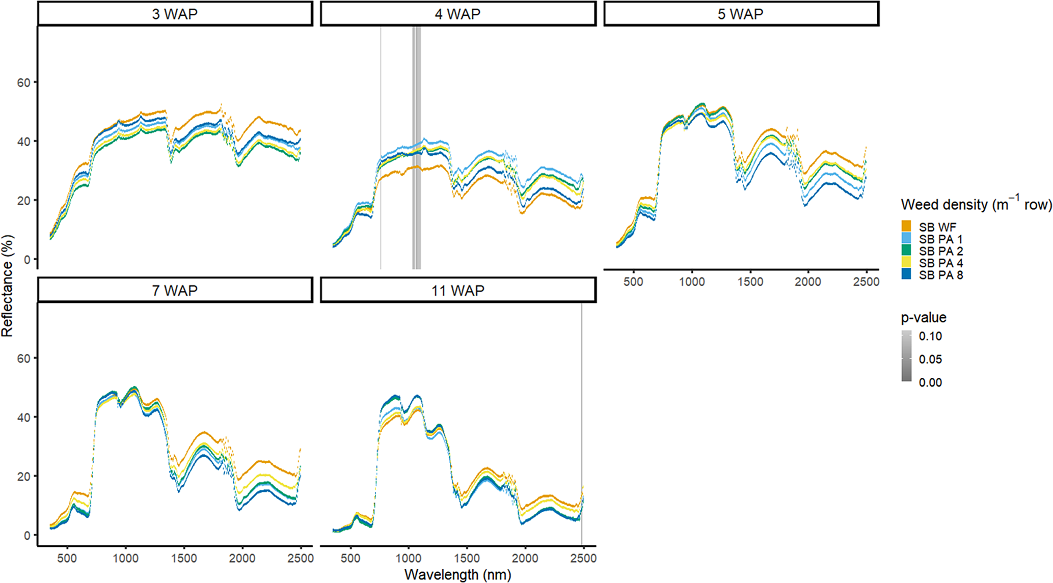
Figure 9. Spectral reflectance for all Amaranthus palmeri (PA) densities with soybean (SB) and a weed-free control (SB WF), grouped by weeks after planting (WAP), at the Horticultural Crops Research Station, Clinton, NC, 2016.
Table 2. Weeks after planting (WAP), date when spectral measurements were taken, growing degree days (GDD), mean plant phenology, and mean plant height across treatments in soybean in 2016 and 2017 at Horticultural Crops Research Station, Clinton, NC.

a Plant phenology based on the BBCH scale (Meier Reference Meier2018).
b Growing Degree Day (GDD) calculated using a base temperature of 10 C.
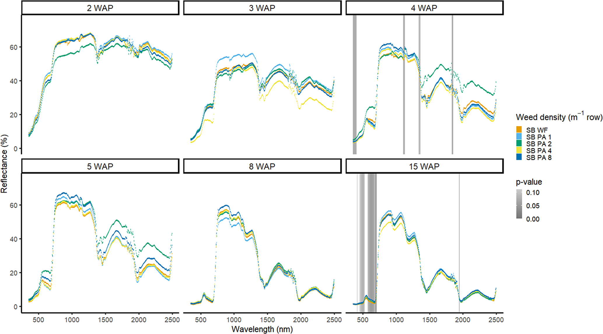
Figure 10. Spectral reflectance for all Amaranthus palmeri (PA) densities with soybean (SB) and a weed-free control (SB WF), grouped by weeks after planting (WAP), at the Horticultural Crops Research Station, Clinton, NC, 2017.
Weed biomass reduction in soybean is likely the reason for poor discrimination of weed species and density (Basinger et al. Reference Basinger, Jennings, Monks, Jordan, Everman, Hestir, Bertucci and Brownie2019). This study showed that weed biomass tended to be significantly greater when not grown with soybean and tended to increase with increasing density. This is likely to be a significant contributing factor to the limited spectral differences seen in the present study. Furthermore, increased leaf layers due to the multi-scaffold branched trifoliate leaves produce many leaf layers, increasing radiative transfer for soybean. This type of structure is similar to that of A. palmeri, making the differentiation of the two species difficult. Amaranthus palmeri was detected in this system when the canopy became established more quickly than soybean and was detectable in the VIS and NIR. Amaranthus palmeri was more readily detected at low densities due to a quickly establishing tall broadleaf canopy that was present above the soybean canopy. However, once the soybean canopy became established, determination of A. palmeri density became more difficult due to the increased leaf area of the crop.
Digitaria sanguinalis was difficult to detect in soybean, and soybean did not allow for large numbers of D. sanguinalis leaves to emerge through the soybean canopy. Detection of D. sanguinalis occurred during the onset of this weed’s reproductive structures, which were able to protrude through the soybean canopy (Figure 11).
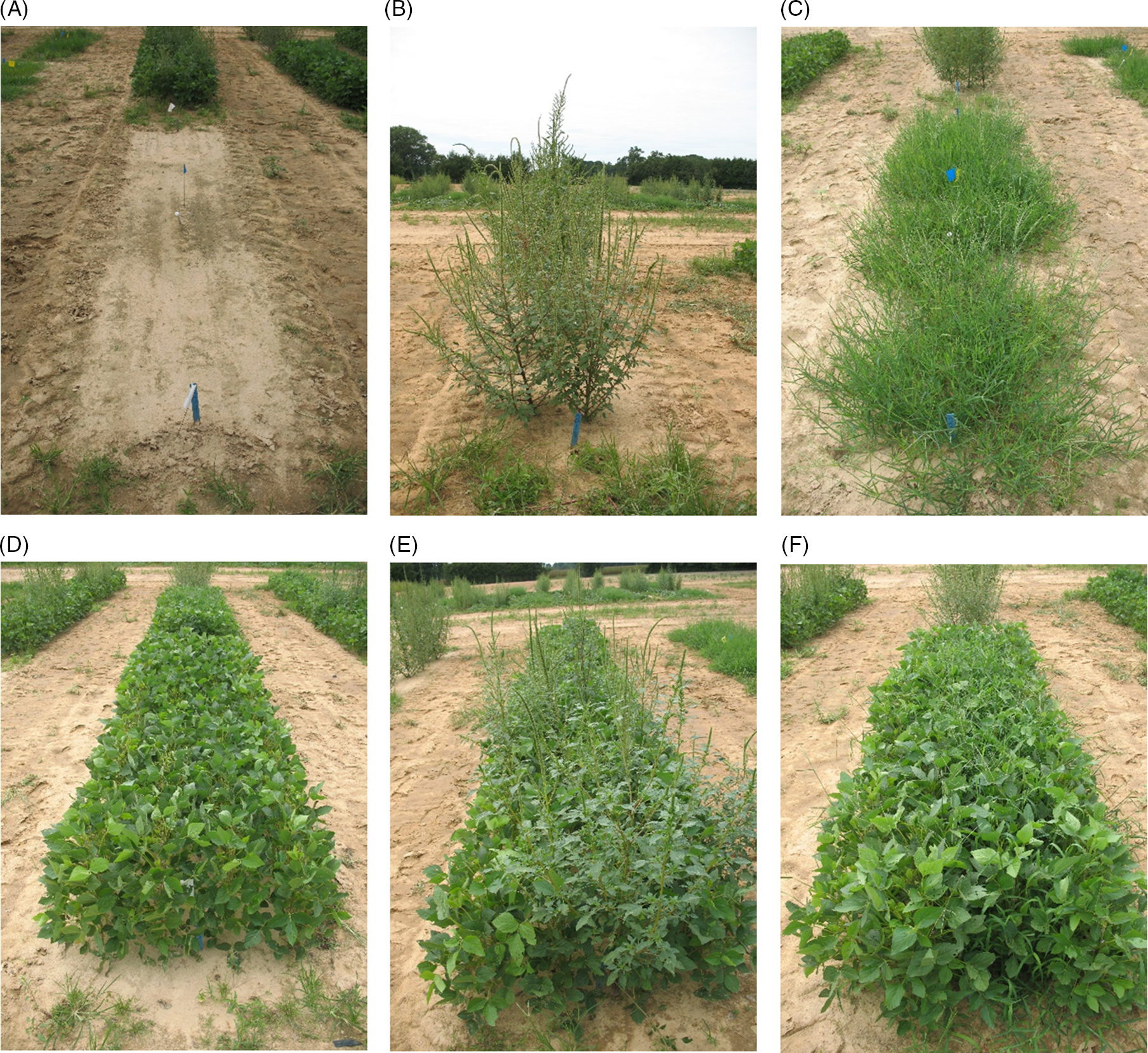
Figure 11. Visual representation of plant structure and growth of weeds with and without soybean: (A) bare ground, (B) Amaranthus palmeri, (C) Digitaria sanguinalis, (D) soybean, (E) soybean and A. palmeri, (F) soybean and D. sanguinalis. All pictures with weeds represent the highest weed density of each species tested.
Estimation of plant density using hyperspectral remote sensing has been successful (Shafian et al. Reference Shafian, Rajan, Schnell, Bagavathiannan and Valasek2018; Thorp et al. Reference Thorp, Steward, Kaleita and Batchelor2008). Detection of A. palmeri occurred early in the season due to rapid biomass accumulation, as seen in previous research (Horak and Loughlin Reference Horak and Loughlin2000). Digitaria sanguinalis was slower establishing a canopy, which made it more difficult to detect early season. Density differentiation between weed-free and lower weed densities has been demonstrated in soybean by others (Koger et al. Reference Koger, Shaw, Reddy and Bruce2004b). However, these differences were not detectable in the presence of soybean in large regions of spectra.
Weeds without Soybean
Detection of weed density without a crop present was more consistent in identifying large portions of spectra that allowed for density discrimination. Detection of both weeds, when compared with the bare-ground control, occurred earlier for both species when density was highest. In 2016, when soybean was not present, D. sanguinalis had more spectra distinguishable based on density at 5 to 11 WAP (Figure 12). Interestingly, it was not until 5 WAP that D. sanguinalis could be distinguished from bare ground, and then only in the VIS regions. Furthermore, for spectral reflectance in the VIS, SWIR1, and SWIR2, the only regions where differences were detectable, reflectance magnitude was related to D. sanguinalis density, with greater densities (4 and 16 plants m−2) having greater spectral absorbance from 7 to 11 WAP. This is somewhat problematic, as the D. sanguinalis plants were quite large at 20-cm tall, having at least 3 internodes visible (Table 2), making it challenging to control at this size. In 2017, when soybean was not present, differences in D. sanguinalis density were noted at 3 WAP on the red edge and the SWIR2 (Figure 13). However, more spectra were differentiable at 4 and 5 WAP and in the blue and longer SWIR spectra. At 3 to 8 WAP, the trend of greater absorbance with greater density was similar to that seen in 2016, indicating that there were greater differences in plant biomass during this period when compared with the bare-ground plots. By 8 and 15 WAP, VIS, SWIR1, and SWIR2 regions had greater absorption than bare-ground plots due to the presence of D. sanguinalis biomass. By 15 WAP, the magnitude between spectra decreased because of the onset of senescence in D. sanguinalis at this reading date.

Figure 12. Spectral reflectance for all Digitaria sanguinalis (LC) densities without soybean (No SB) and a bare ground control (No SB BG), grouped by weeks after planting (WAP), at the Horticultural Crops Research Station, Clinton, NC, 2016.
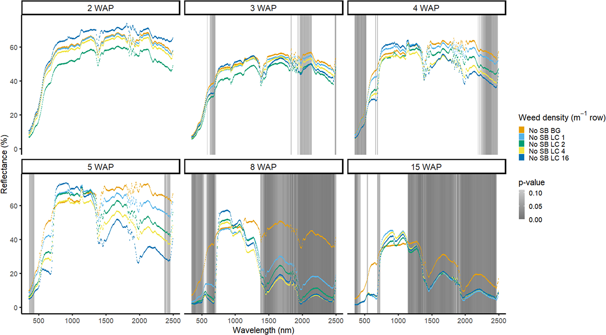
Figure 13. Spectral reflectance for all Digitaria sanguinalis (LC) densities without soybean (No SB) and a bare-ground control (No SB BG), grouped by weeks after planting (WAP), at the Horticultural Crops Research Station, Clinton, NC, 2017.
Amaranthus palmeri detection occurred at a similar timing to that of D. sanguinalis for each year. In 2016, differences in A. palmeri density were only noted at 5 WAP (VIS and SWIR2) and 11 WAP (VIS, SWIR1, and SWIR2) (Figure 14). In 2017, differences occurred earlier in the season (3 WAP) and across more spectra (Figure 15). Many of the differences between A. palmeri density were in the VIS, with late-season (8 and 15 WAP) differences occurring across most spectra in the SWIR1 and SWIR2 regions.
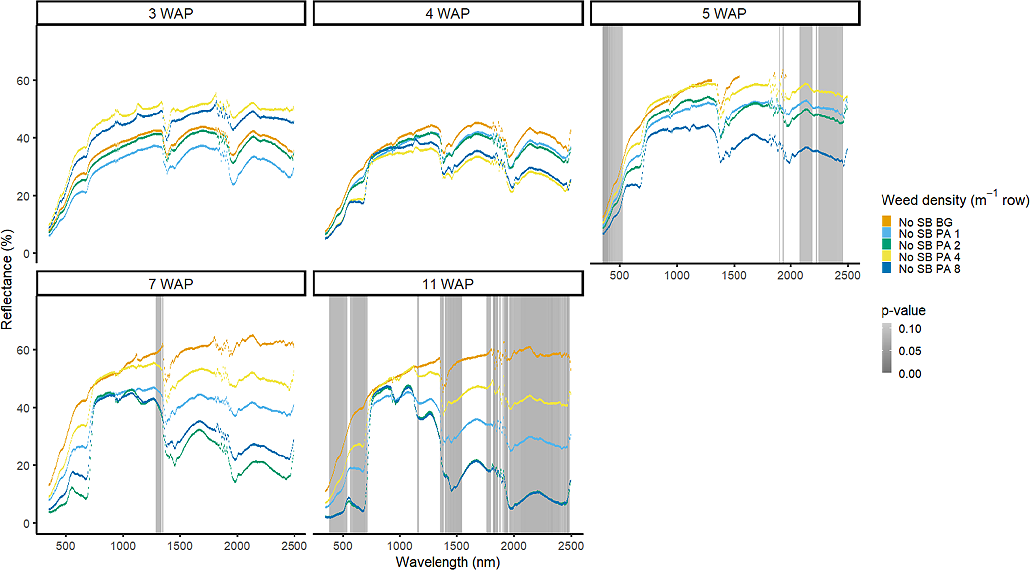
Figure 14. Spectral reflectance for all Amaranthus palmeri (PA) densities without soybean (No SB) and a bare-ground control (No SB BG), grouped by weeks after planting (WAP), at the Horticultural Crops Research Station, Clinton, NC, 2016.
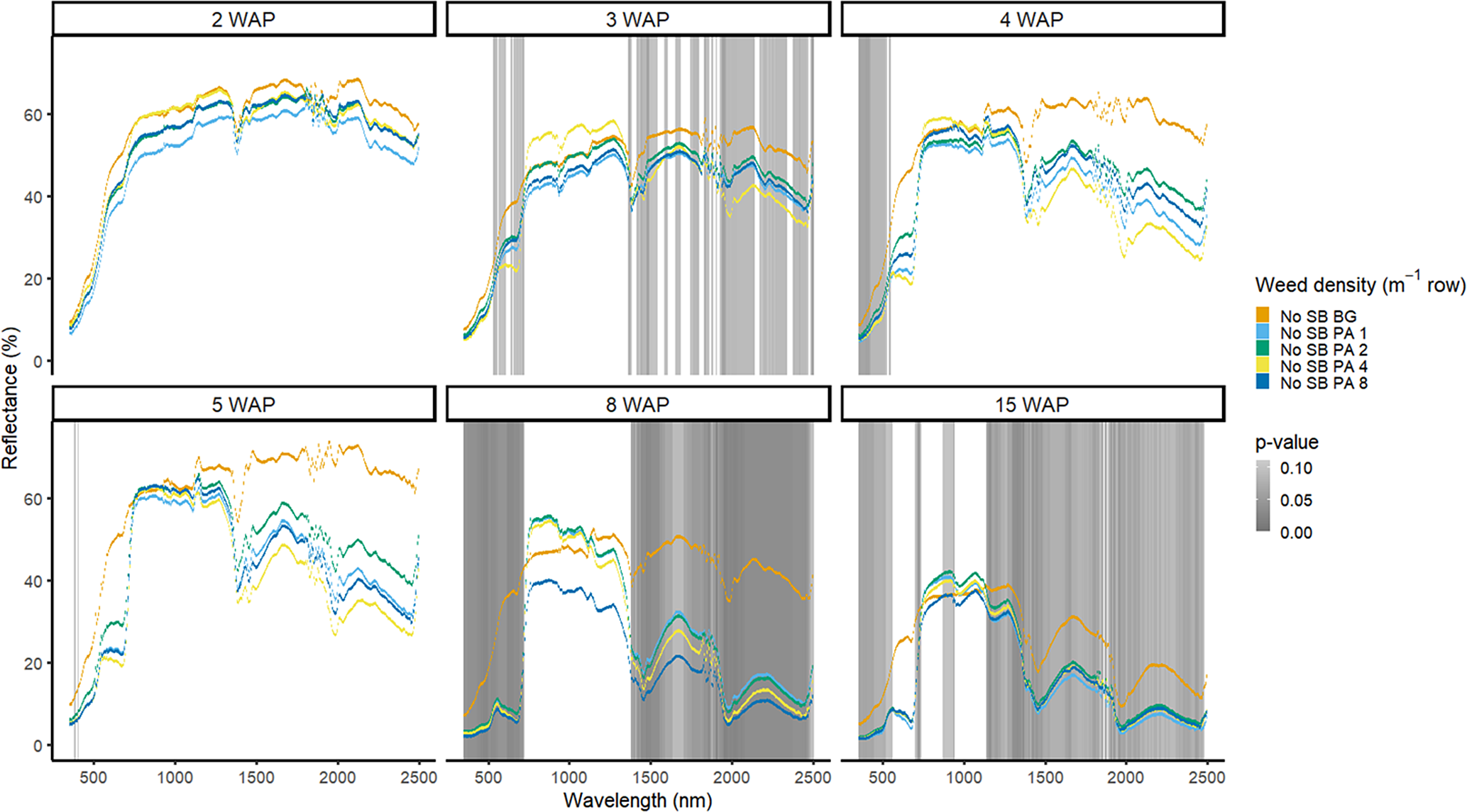
Figure 15. Spectral reflectance for all Amaranthus palmeri (PA) densities without soybean (No SB) and a bare-ground control (No SB BG), grouped by weeks after planting (WAP), at the Horticultural Crops Research Station, Clinton, NC, 2017.
Weed and Crop Phenology
The phenology of crop and weed species was not affected by crop presence/absence and weed density, as phenological differences between densities were not noted (Table 2). Annual differences in phenological timing were different between years as defined by Meier (Reference Meier2018). At the earliest data-collection dates across years and cropping systems, weed species and density did not have established canopies and could not be differentiated from either weed-free or bare-ground treatments. Rapid establishment of weed species canopies, especially with A. palmeri, leads to increased absorption in VIS early in the season. Similarly, early detection of D. sanguinalis was due to increased canopy coverage of higher-density treatments. The establishment of weed canopy was critical to the differentiation between crop species and density.
Weed species phenology did not differ between densities, but overall weed biomass and height did change due to interspecific competition with each crop and intraspecific competition due to increased weed density (Basinger et al. Reference Basinger, Jennings, Monks, Jordan, Everman, Hestir, Bertucci and Brownie2019). Higher weed density tended to fill out a canopy more quickly, but individual plants tended to be smaller overall than at lower weed densities. Lower-density weed species toward the end of the season in each year tended to have greater canopy density per plant but were similar overall at higher plant densities. Higher densities of weed species tended to have greater absorption in the VIS, SWIR1, and SWIR2 earlier in the season. As canopies of lower-density treatments became established, differences between weed densities were observed at fewer SWIR1 and SWIR2 spectra but continued in the VIS region. Plant phenology is important for the differentiation and detection of weed species. Phenology is not often considered in studies using remote sensing for species discrimination (Santos et al. Reference Santos, Khanna, Hestir, Greenberg and Ustin2016; Schmidt and Skidmore Reference Schmidt and Skidmore2003), but spectral reflectance does change with changing crop phenology (Basinger et al. Reference Basinger, Jennings, Hestir, Monks, Jordan and Everman2020; Vina et al. Reference Vina, Gitelson, Rundquist, Keydan, Leavitt and Schepers2004). Phenology and biophysical characteristics are inherently linked with one another and are correlated with hyperspectral reflectance (Lausch et al. Reference Lausch, Salbach, Schmidt, Doktor, Merbach and Pause2015). Changing plant phenology can have effects on internal leaf structure and chlorophyll concentration, which could explain some of the overall changes in spectra during each growing season (Poorter et al. Reference Poorter, Niinemets, Poorter, Wright and Villar2009; Slaton et al. Reference Slaton, Raymond Hunt and Smith2001) High temporal data collection in the early season is important for the detection of weed species, as plant phenology changes rapidly during this time. Early-season detection is also important in agricultural systems, because weed management strategies are most effective when weeds are small.
This study aimed to elucidate spectral changes in a soybean crop with varying densities of two weed species across several phenological time points. The study showed that spectral reflectance is dynamic throughout the season and between seasons, with the magnitude and shape of each spectrum changing in some parts of the measured spectra, while other spectra were similar across observation dates despite differences in treatments (bare ground, weed-free soybean, density of D. sanguinalis or A. palmeri). These variations in absorbance, reflectance, and magnitude changes over the season could be used as targets to assess plant phenology and/or plant density. Spectral changes were seen more when there were differences in the amount of vegetation present, indicating that areas of greater weed populations could be spectrally distinguished from lower-density areas of the same species. Furthermore, plants that are more phenologically separate in terms of biomass production and reproduction and overall canopy structure can provide opportunities for spectral differentiation.
Given that much of the spectral differentiation in this study was in the VIS region, there is a significant opportunity to leverage these differences using standard RGB photographs coupled with machine learning to assist in the differentiation of crop and weed species. However, there are several spectral in the SWIR1 and SWIR2 regions that could be further utilized for differentiation of species and weed density. Leveraging these additional spectra may provide opportunities to further improve the discrimination of plant species using artificial intelligence. Furthermore, understanding the impact of variations in magnitude of absorbance and reflectance of certain spectra as plant phenology changes could provide additional insight into building more accurate algorithms and sensor platforms for use in agricultural systems.
In this study, plant phenology was important in the detection and differentiation of weed species, and it should be incorporated in future studies. Additional challenges of identification of site-specific weed management include the development of an appropriate threshold to determine when weed management is necessary and the methods to be used to control weeds. This study focused on the detection and differentiation of individual weed species that were not part of a weed species complex but utilized reflectance spectra to differentiate between crops and weeds. The weed species complex should be considered, as this situation more accurately reflects the natural occurrence of weeds in agricultural systems.
Acknowledgments
The authors would like to thank the staff at the Horticultural Crops Research Station, Clinton, NC, for their help in the maintenance and use of equipment and assistance with the studies. Special thanks to Matthew Waldschmidt, Cole Smith, Matthew Bertucci, Spencer Monaco, Catherine Monaco, Andrea Genna, Anna Wyngaarden, Rachel Berube, and Lauren Deans for their assistance in study maintenance and data collection. Thanks to Christiana Ade and Megan Amanatides from the Hestir Lab at North Carolina State University for their guidance and assistance in data processing. No conflicts of interest have been declared.


 Open access