


1. Introduction
This paper proposes a method to drastically reduce the required number of legs degrees-of-freedom (DOFs), for bipedal robots and lower-limb exoskeletons, that is needed for walking. The proposed approach will release more DOFs into the null space and will allow more tasks to be performed simultaneously while walking, that is, balancing against gravity, avoiding obstacles, shifting the center of mass, etc. Normally, the greater the DOFs of a robot, the more tasks it can accommodate. However, this work will show that given a physical robot with a fixed number of DOFs, the available number of DOFs to perform certain tasks also depends on the choice of reference frames used to perform the robot control.
Bipedal robots are important because they offer autonomous, human-like mobility in an environment built for human activities [Reference Collins, Ruina, Tedrake and Wisse1,Reference Höhn and Gerth2]. In an indoor environment, for example, they are a useful tool for moving around objects, interacting with humans, and assisting to collaborate with humans in simple tasks [Reference Bhounsule, Zamani, Krause, Farra and Pusey3,Reference Luo, Su, Ruan, Zhao, Kim, Sentis and Fu4]. They have a tremendous future promise in terms of assisting humans as a robotic laborer, maid, and elderly care. In the case of lower-limb exoskeletons, there is a huge promise in assistance to human walking, instead of using a wheelchair, and for leg rehabilitation [Reference Moreno, Figueiredo and Pons5,Reference Bass, Morin, Vermette, Aubertin-Leheudre and Gagnon6].
Compared to bipedal robots, lower-limb exoskeletons do not move autonomously but are attached to human legs to assist humans in walking. They rely on communication from their human users to provide the needed assistance in the walking execution. However, bipedal robots and robot exoskeletons share the same principle of motion: that of providing foot movement with respect to the ground and balancing its mechanical structure so as not to fall against gravity. This is the kind of motion control that is discussed in this paper.
1.1. Reduction of the required DOFs
In general, the foot of a bipedal robot is controlled to move w.r.t. a fixed reference frame, which is either a body frame or a world frame. This approach is what is normally used in earlier studies, where a sample of them is shown in Table 1. This kind of foot movement is referred to as absolute foot motion, that is, the foot movement w.r.t. an absolute reference frame. To control the absolute foot position (and disregarding orientation) of a bipedal robot, one would need at least 3-DOFs for each leg. With the additional task to balance against gravity, at least one more leg DOF is needed to achieve the required leg posture in the null space. This sums up to a minimum of 4-DOFs for each leg in bipedal robots in controlling absolute feet position.
Table 1. A summary of some previous work in bipedal robot walking published in journals
1 Int. J. Robot. Res.
2 IEEE Trans. Robot.
3 IEEE Trans. Autom. Control
4 IEEE Trans. Ind. Electron.
5 IEEE Trans. Cont. Syst. Technol.
6 IEEE Trans. Syst., Man, Cybern., Syst.
7 J. Intell. Robot. Syst
The proposed method presented in this work controls one foot to move w.r.t. the reference frame of the other foot, that is, w.r.t. a moving reference frame. This kind of foot movement is referred to as relative feet motion. However, to proceed with this control strategy, the bipedal robot has to be controlled holistically as a single robot. Thus, to control the relative feet position (and disregarding orientation), one would need at least a total of 3-DOFs for the entire bipedal robot. With the additional task to balance against gravity, one more DOF is needed to achieve the required posture in the null space. Thus, the entire bipedal robot requires a total of 4-DOFs, with each leg having 2-DOFs. This example shows that using relative feet position requires half of the required leg DOFs compared to using absolute feet position.
Figure 1 shows a bipedal robot with 3-DOFs in each leg. If we control its absolute feet motion, there will be no extra joints to balance against gravity. But if we control its relative feet motion, there will be three extra joints that will allow us to balance against gravity, avoid obstacles, etc.
1.2. The relative Jacobian versus absolute Jacobian
To implement the necessary control for the two approaches discussed above, a relative Jacobian is used to control the relative feet motion. The usual Jacobian, which is used to control the robot end effector w.r.t. its base, will be called absolute Jacobian. An absolute Jacobian is used to control the absolute foot motion.
The first expression of a relative Jacobian denoted $\mathbf{J}_R$
, was shown in ref. [Reference Lewis and Maciejewski7] for two cooperating manipulators but the final expression was not modular. The first expression of modular relative Jacobian for dual arms is shown in ref. [Reference Jamisola and Roberts8], and with dynamics information included is shown in ref. [Reference Jamisola, Kormushev, Roberts and Caldwell9]. An impedance control using relative Jacobian with dynamics was shown in ref. [Reference Lee, Chang and Jamisola10] for a dual-arm robot, with each arm having 6-DOFs, but the Jacobian expression was not modular.
$\mathbf{J}_R$
, was shown in ref. [Reference Lewis and Maciejewski7] for two cooperating manipulators but the final expression was not modular. The first expression of modular relative Jacobian for dual arms is shown in ref. [Reference Jamisola and Roberts8], and with dynamics information included is shown in ref. [Reference Jamisola, Kormushev, Roberts and Caldwell9]. An impedance control using relative Jacobian with dynamics was shown in ref. [Reference Lee, Chang and Jamisola10] for a dual-arm robot, with each arm having 6-DOFs, but the Jacobian expression was not modular.
1.3. Claimed contributions
The first advantage of the proposed approach is the use of relative feet movement in bipedal walking control. To the best of our knowledge, this study is the first of its kind in controlling bipedal walking. It is implemented through the use of a relative Jacobian, which results in a drastic reduction of the required DOFs for bipedal robots.
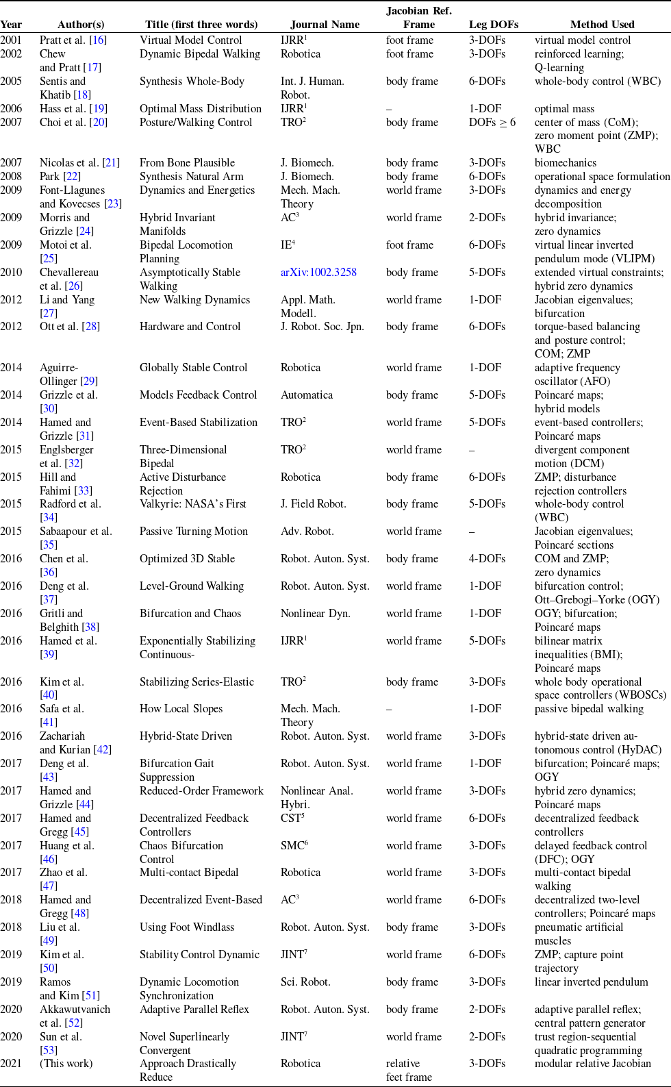
Figure 1. The bipedal robot in Gazebo simulation. Each leg has 3-DOFs. The right leg is labeled “Leg A”, while the left leg is labeled “Leg B”. The reference frames are shown such that the axis with an arrowhead (colored blue) is the z-axis, following the right-hand rule. The hip joints rotate around the z-axis of frames $\{1\}$
and
$\{1\}$
and $\{3\}$
, while frames
$\{3\}$
, while frames $\{2\}$
and
$\{2\}$
and $\{4\}$
are attached to the feet and are fixed. All joints are moving and are rotating about the z-axis (blue arrow), except the fixed joints of frames
$\{4\}$
are attached to the feet and are fixed. All joints are moving and are rotating about the z-axis (blue arrow), except the fixed joints of frames $\{2\}$
and
$\{2\}$
and $\{4\}$
. A video of the bipedal robot is shown here: https://youtu.be/PjGLETk81_g.
$\{4\}$
. A video of the bipedal robot is shown here: https://youtu.be/PjGLETk81_g.
The second advantage is its holistic control. This is important because the expressions related to the control of a single redundant robot can now be applied to bipedal robots. This means that bipedal walking can now be implemented using only two major controllers: one for the relative feet motion and another for the null-space leg posture. This also means that task prioritization can now be implemented very strictly just like a single manipulator controller.
The third advantage is the modularity of expression of the proposed approach. That is, the expression consists of identifiable components of each of the absolute Jacobian for each leg. This affords independent control for each leg as a component of the holistic control of the entire bipedal robot. In addition, when legs are changed, only the absolute Jacobian components (and their corresponding transformation matrices) are to be replaced without the need to rederive a completely new formulation of the relative Jacobian.
2. Previous approaches in bipedal robot control
In this section, we show a summary of some previous work published in journal publications regarding bipedal robot walking. This is shown in Table 1. The journal papers range from the years 2001 to 2019. The first column in the table lists the authors, while the title column shows the first three words of the paper title. Journal names are abbreviated according to listed standards from publishers. The table presents previous approaches in bipedal walking in terms of (a) frame of reference of the Jacobian used, (b) the number of joints in each leg, and (c) the method used in controlling bipedal motion. These are critical information toward evaluating the proposed modular relative Jacobian approach. Most of the work in bipedal walking used the body frame or world frame as the reference frame of the Jacobian. This influences the kind of control approach used in bipedal walking. We discuss below some of the more prominent methods of controlling bipedal walking below.
Method 1. Center of Mass (CoM) approach normally is paired with the Zero Moment Point (ZMP) such that the Jacobian is expressed w.r.t. the CoM point on the body, and the ZMP is computed from the torques generated based on the motion of CoM w.r.t. the ground.
Method 2. In the case of the whole-body control (WBC), different tasks, postures, and constraints, with their corresponding Jacobians, have different hierarchies of execution. All torques are added together at the joint-level control. In this case, the different Jacobians are expressed at their corresponding body frames. Each of the legs has 6-DOFs.
Method 3. The inverted pendulum approach uses the foot (base) frame as the reference frame for the Jacobian matrix. The center of gravity position and velocity is controlled to balance against gravity, as well as to ensure necessary torques are delivered on time to counter the gravitational force that is pulling the body downward. This approach is normally implemented on a 1-DOF leg platform.
Method 4. Ott–Grebogi–Yorke (OGY) is used to stabilize gait bifurcation. Jacobian is expressed at CoM. Pioncaré map is used to transform the continuous walking process, this is also known as the stride function. This approach normally studies 1-DOF leg platforms.
Method 5. The method of zero dynamics usually uses Jacobian linearization about a fixed point and deals with the invariance of results in the presence of disturbances. The reference frame of the Jacobian can be in the body or world frame. The legs can have 2-, 3-, or 4-DOFs.
Method 6. The operational space formulation in the bipedal robot is similar to the WBC. The reference frame of the Jacobian is in the body and each leg has 6-DOFs.
Method 7. Often used with gait bifurcation, gait stability is monitored through a threshold of the eigenvalues of the Jacobian. The frame of reference is the world frame and is usually implemented on a 1-DOF leg.
Overall, the major challenges on bipedal walking include gait stability, holistic control to address the issue of the hierarchy of motion execution, and the legs DOFs that will allow bipedal motion in full space. This paper does not address the issue of gait stability, but only addresses the issue of holistic control, the hierarchy of motion execution, and the legs DOFs in bipedal motion.
From Table 1, our proposed approach of relative reference frames is the only method that accommodates null-space control when each leg has 6-DOFs and the foot movement is controlled in the full space. This is also true when the foot movement is controlled in full-position control and each leg has 3-DOFs. Other recent studies in bipedal walking include stability constraints [Reference Sanchez, Wan, Kanehiro and Harada11], RRT-based motion planner [Reference Wasielica and Belter12], impact dynamics [Reference Luo, Xia and Zhu13,Reference Mobinipour14], and tactile feedback [Reference Guadarrama Olvera, Dean Leon, Bergner and Cheng15].
3. The modular relative jacobian for bipedal robots
The modular relative Jacobian formulation [Reference Jamisola and Roberts8] is shown here for bipedal robot implementation. Figure 1 shows the reference frames assignment in a bipedal robot. The labeled reference frames are the hip and foot frames of the bipedal robot. These correspond to the base and end effector frames, respectively, of the absolute Jacobian for each leg. Note that all joints are rotating about the z-axis (blue arrow) except those attached to the fixed reference frames $\{2\}$
and
$\{2\}$
and $\{4\}$
. For leg A, its absolute Jacobian is
$\{4\}$
. For leg A, its absolute Jacobian is $\mathbf{J}_A={}^1\mathbf{J}_2$
. This means that the base frame for this Jacobian is frame {1} and its end effector frame is frame {2}. On the other hand, the absolute Jacobian for leg B is
$\mathbf{J}_A={}^1\mathbf{J}_2$
. This means that the base frame for this Jacobian is frame {1} and its end effector frame is frame {2}. On the other hand, the absolute Jacobian for leg B is $\mathbf{J}_B = {}^3\mathbf{J}_4$
, with the base frame {3} and end effector frame {4}. Relative motion is expressed in terms of the motion of frame {4} w.r.t. frame {2}. Or in conventional terms, frame {2} as the base frame and frame {4} as the end effector frame. Thus the relative position and orientation can be expressed as,
$\mathbf{J}_B = {}^3\mathbf{J}_4$
, with the base frame {3} and end effector frame {4}. Relative motion is expressed in terms of the motion of frame {4} w.r.t. frame {2}. Or in conventional terms, frame {2} as the base frame and frame {4} as the end effector frame. Thus the relative position and orientation can be expressed as, ${}^2\mathbf{x}_4=[{}^2\mathbf{p}_4,{}^2\boldsymbol{\Phi}_4]$
, where
${}^2\mathbf{x}_4=[{}^2\mathbf{p}_4,{}^2\boldsymbol{\Phi}_4]$
, where ${}^2\mathbf{p}_4$
is relative position and
${}^2\mathbf{p}_4$
is relative position and ${}^2\boldsymbol{\Phi}_4$
is relative orientation.
${}^2\boldsymbol{\Phi}_4$
is relative orientation.
Using the above convention, the modular relative Jacobian, $\mathbf{J}_R$
, can be expressed in terms of the absolute Jacobians for each leg, as shown in [Reference Jamisola and Mastalli54], that is,
$\mathbf{J}_R$
, can be expressed in terms of the absolute Jacobians for each leg, as shown in [Reference Jamisola and Mastalli54], that is,
 \begin{equation}\mathbf{J}_R =\left[\begin{matrix}-{}^2\Psi_4 {}^2\Omega_1 {}^1\mathbf{J}_2&\quad \quad & {}^2\Omega_3 {}^3\mathbf{J}_4\end{matrix}\right]\end{equation}
where
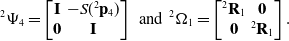 \begin{equation}{}^2\Psi_4 =\left[\begin{matrix}\mathbf{I} & -S({}^2\mathbf{p}_4) \\\mathbf{0} & \mathbf{I} \end{matrix}\right] \;\;\mbox{and}\;\;{}^2\Omega_1 =\left[\begin{matrix}{}^2\mathbf{R}_1 & \mathbf{0} \\\mathbf{0} & {}^2\mathbf{R}_1 \end{matrix}\right].\end{equation}
In general, $\mathbf{J}_A \in \mathbb{R}^{6\times n_A}$
and
$\mathbf{J}_A \in \mathbb{R}^{6\times n_A}$
and $\mathbf{J}_B \in \mathbb{R}^{6\times n_B}$
, where
$\mathbf{J}_B \in \mathbb{R}^{6\times n_B}$
, where $n_A$
is the number of joints for leg A and
$n_A$
is the number of joints for leg A and $n_B$
is the number of joints for leg B;
$n_B$
is the number of joints for leg B; ${}^2\Psi_4, {}^2\Omega_1, {}^2\Omega_3 \in \mathbb{R}^{6\times 6}$
; and
${}^2\Psi_4, {}^2\Omega_1, {}^2\Omega_3 \in \mathbb{R}^{6\times 6}$
; and $\mathbf{J}_R \in \mathbb{R}^{6 \times ({n_A+n_B})}$
. The symbol
$\mathbf{J}_R \in \mathbb{R}^{6 \times ({n_A+n_B})}$
. The symbol ${}^2\boldsymbol{\Omega}_3= f({}^2\mathbf{R}_3)$
is expressed as in (2). The relative position vector
${}^2\boldsymbol{\Omega}_3= f({}^2\mathbf{R}_3)$
is expressed as in (2). The relative position vector ${}^2\mathbf{p}_4$
is expressed as
${}^2\mathbf{p}_4$
is expressed as
 \begin{equation}{}^2\mathbf{p}_4 = {}^2\mathbf{p}_1 + {}^2\mathbf{R}_1 {}^1\mathbf{p}_3 + {}^2\mathbf{R}_3 {}^3\mathbf{p}_4.\end{equation}
To further simplify the expressions we introduce
 \begin{equation}\begin{matrix}\mathbf{Q}_A = -{}^2\Psi_4 {}^2\Omega_1 & \mbox{and} &\mathbf{Q}_B = {}^2\Omega_3\end{matrix}\end{equation}
such that the modular relative Jacobian becomes
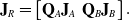 \begin{equation}\mathbf{J}_R =\left[\begin{matrix}\mathbf{Q}_A \mathbf{J}_A & \mathbf{Q}_B \mathbf{J}_B\end{matrix}\right].\end{equation}
In this implementation, we only intend to verify the accuracy of the kinematics model of the relative Jacobian for bipedal robots. Thus, we do not include the full dynamics information but added only the gravity term to the pure kinematics controller. This strategy will emphasize the results of our proposed solution on reduction of legs DOFs, holistic control, strict task prioritization, and modularity of expression. The total torques supplied to the joints are
 \begin{equation}\boldsymbol{\tau}_T =\mathbf{J}_R^T {\ddot{\textbf{x}}}_R +(\mathbf{I} - \mathbf{J}_R^T \mathbf{J}_R^{+T}) \boldsymbol{\tau}_O +\mathbf{g}_T.\end{equation}
The first term is the end effector motion, the second term is the null-space motion, and the last term is the gravitational term. Furthermore, $\boldsymbol{\tau}_T =\left[\begin{matrix}\tau_A^T & \tau_B^T\end{matrix}\right]^T$
where
$\boldsymbol{\tau}_T =\left[\begin{matrix}\tau_A^T & \tau_B^T\end{matrix}\right]^T$
where $\tau_A^T\in R^{n_A}$
and
$\tau_A^T\in R^{n_A}$
and $\tau_B^T\in R^{n_B}$
,
$\tau_B^T\in R^{n_B}$
, $\mathbf{g}_T =\left[\begin{matrix}\mathbf{g}_A^T & \mathbf{g}_B^T\end{matrix}\right]^T$
where
$\mathbf{g}_T =\left[\begin{matrix}\mathbf{g}_A^T & \mathbf{g}_B^T\end{matrix}\right]^T$
where $\mathbf{g}_A^T \in R^{n_A}$
and
$\mathbf{g}_A^T \in R^{n_A}$
and $\mathbf{g}_B^T \in R^{n_B}$
,
$\mathbf{g}_B^T \in R^{n_B}$
, ${\ddot{\textbf{x}}}_R\in R^{6}$
, and
${\ddot{\textbf{x}}}_R\in R^{6}$
, and $\boldsymbol{\tau}_O \in R^{n_A+n_B}$
. Subscript A corresponds to leg A and subscript B corresponds to leg B and subscript T means total, that is, corresponding to both A and B. The symbol
$\boldsymbol{\tau}_O \in R^{n_A+n_B}$
. Subscript A corresponds to leg A and subscript B corresponds to leg B and subscript T means total, that is, corresponding to both A and B. The symbol $\mathbf{g}$
is the gravity term,
$\mathbf{g}$
is the gravity term, ${\ddot{\textbf{x}}}_R$
is the relative acceleration,
${\ddot{\textbf{x}}}_R$
is the relative acceleration, $\boldsymbol{\tau}_O$
is the null-space control, and n is the leg DOFs.
$\boldsymbol{\tau}_O$
is the null-space control, and n is the leg DOFs.
4. Implementation of bipedal walking
It should be emphasized that in this implementation, there are two major controllers to perform bipedal walking: (1) the controller for the relative feet motion and (2) the controller to balance against gravity. The first controller corresponds to the world space control, while the second controller corresponds to the null-space posture control. To verify the proposed approach, we simulate a bipedal robot in Gazebo with ROS. Kinematics and dynamics information was derived using KDL libraries in ROS. The absolute Jacobians $\mathbf{J}_A$
and
$\mathbf{J}_A$
and $\mathbf{J}_B$
for the legs were read directly from KDL, together with the information for the gravitational terms
$\mathbf{J}_B$
for the legs were read directly from KDL, together with the information for the gravitational terms $\mathbf{g}_A$
and
$\mathbf{g}_A$
and $\mathbf{g}_B$
. Because the implementation shown here is purely kinematics (with gravity compensation), its results are expected to be not as robust as when the dynamics information is modeled or compensated. But these results are shown to demonstrate the efficacy of the proposed controller and that it is sufficient to guarantee bipedal walking at a much-reduced DOFs of the robot legs.
$\mathbf{g}_B$
. Because the implementation shown here is purely kinematics (with gravity compensation), its results are expected to be not as robust as when the dynamics information is modeled or compensated. But these results are shown to demonstrate the efficacy of the proposed controller and that it is sufficient to guarantee bipedal walking at a much-reduced DOFs of the robot legs.
The acceleration term, ${\ddot{\textbf{x}}}_R$
, in (6) is replaced by the control equation
${\ddot{\textbf{x}}}_R$
, in (6) is replaced by the control equation $\mathbf{u}$
such that the joints torque commands to the robot become,
$\mathbf{u}$
such that the joints torque commands to the robot become,
 \begin{equation}\boldsymbol{\tau}_T = \mathbf{J}_R^T \mathbf{u} +(\mathbf{I} - \mathbf{J}_R^T \mathbf{J}_R^{+T}) \boldsymbol{\nabla} \mathbf{z} +\widetilde{\mathbf{g}}_T\end{equation}
where $\widetilde{\square}$
on top of a symbol representing a physical parameter means that it is the estimate of that parameter,
$\widetilde{\square}$
on top of a symbol representing a physical parameter means that it is the estimate of that parameter, $\mathbf{u}$
is the relative position control in the world space, and
$\mathbf{u}$
is the relative position control in the world space, and $\boldsymbol{\nabla} \mathbf{z}$
is the posture control. In this implementation, we only control the relative feet position
$\boldsymbol{\nabla} \mathbf{z}$
is the posture control. In this implementation, we only control the relative feet position ${}^2\mathbf{p}_4$
, with no control on relative feet orientation
${}^2\mathbf{p}_4$
, with no control on relative feet orientation ${}^2\boldsymbol{\Phi}_4$
. Next, we will show how we control the world space relative feet position through
${}^2\boldsymbol{\Phi}_4$
. Next, we will show how we control the world space relative feet position through $\mathbf{u}$
, and the corresponding posture to balance against gravity
$\mathbf{u}$
, and the corresponding posture to balance against gravity $\nabla\mathbf{z}$
.
$\nabla\mathbf{z}$
.
4.1. World space relative position control
A simple PD control is used to control both the world space relative position, as well as the null-space posture control. The world space relative position control $\mathbf{u}$
from (7) can be expressed as
$\mathbf{u}$
from (7) can be expressed as
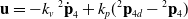 \begin{equation}\mathbf{u} = - k_v\;{}^2{\dot{\textbf{p}}}_4 +k_p ({}^2\mathbf{p}_{4d} - {}^2\mathbf{p}_4)\end{equation}
where the value of the proportional gain $k_p=20$
and the value of the derivative gain
$k_p=20$
and the value of the derivative gain $k_v=0.02$
. Subscript d means desired values. We compute the value of
$k_v=0.02$
. Subscript d means desired values. We compute the value of ${}^2\mathbf{p}_4$
from (3), and the translational velocity
${}^2\mathbf{p}_4$
from (3), and the translational velocity ${}^2{\dot{\textbf{p}}}_4$
is computed by
${}^2{\dot{\textbf{p}}}_4$
is computed by
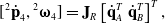 \begin{equation}[{}^2{\dot{\textbf{p}}}_4,{}^2\boldsymbol{\omega}_4]= \mathbf{J}_R\left[\begin{matrix}{\dot{\textbf{q}}}_A^T & {\dot{\textbf{q}}}_B^T\end{matrix}\right]^T,\end{equation}
where $^2\boldsymbol{\omega}_4$
is the relative angular velocity, and
$^2\boldsymbol{\omega}_4$
is the relative angular velocity, and ${\dot{\textbf{q}}}_A$
and
${\dot{\textbf{q}}}_A$
and ${\dot{\textbf{q}}}_B$
are the leg velocities. We set the desired values of the relative position by going through a cycle of alternately putting one foot ahead of the other, that is,
${\dot{\textbf{q}}}_B$
are the leg velocities. We set the desired values of the relative position by going through a cycle of alternately putting one foot ahead of the other, that is,
 \begin{equation}{}^2\mathbf{p}_{4d}=[(-1)^{c}0.2 a \;\;(-1)^{c}0.2\;\;0.25]^T\end{equation}
where $c\in{N}$
that increments every
$c\in{N}$
that increments every $t=0.5s$
and
$t=0.5s$
and $a\in\{1,0\}$
switches between 1 and 0 every
$a\in\{1,0\}$
switches between 1 and 0 every $0.5t$
. Note that Gazebo does not run in real time. Physically this means that at the start of the cycle, the left foot (of leg B) simultaneously lifts and moves forward (w.r.t. the right foot), then touches the ground. In the second half of the cycle, the right foot (of leg A) simultaneously lifts and moves forward (w.r.t. the left foot), then touches the ground.
$0.5t$
. Note that Gazebo does not run in real time. Physically this means that at the start of the cycle, the left foot (of leg B) simultaneously lifts and moves forward (w.r.t. the right foot), then touches the ground. In the second half of the cycle, the right foot (of leg A) simultaneously lifts and moves forward (w.r.t. the left foot), then touches the ground.
4.2. Null-space control
Posture is controlled using the feedback of the IMUs placed at both ends of the hip link connecting the two legs as shown in Fig. 1. In this arrangement, using Fig. 1 frame assignment and labeling the ground as frame {0}, the IMU feedback are ${}^0\mathbf{R}_{1}$
and
${}^0\mathbf{R}_{1}$
and ${}^0\mathbf{R}_{3}$
from frame {1} and frame {3}, respectively. The desired orientation is set to be the orientation of the hip w.r.t. the ground at the initial stage of the walking, that is,
${}^0\mathbf{R}_{3}$
from frame {1} and frame {3}, respectively. The desired orientation is set to be the orientation of the hip w.r.t. the ground at the initial stage of the walking, that is, ${}^0\mathbf{R}_{1d} = {}^0\mathbf{R}_{3d} = \mathbf{I}$
where
${}^0\mathbf{R}_{1d} = {}^0\mathbf{R}_{3d} = \mathbf{I}$
where $\mathbf{I}$
is the identity matrix. By considering the rotation matrix to be
$\mathbf{I}$
is the identity matrix. By considering the rotation matrix to be $\mathbf{R}=[\mathbf{n} \;\mathbf{o} \;\mathbf{a}]$
, a generic orientation control is
$\mathbf{R}=[\mathbf{n} \;\mathbf{o} \;\mathbf{a}]$
, a generic orientation control is
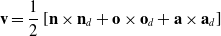 \begin{equation}\begin{split}\mathbf{v}& = \frac{1}{2}\left[{}\mathbf{n}\times {}\mathbf{n}_{d} +{}\mathbf{o}\times {}\mathbf{o}_{d} +{}\mathbf{a}\times {}\mathbf{a}_{d}\right] \\\end{split}\end{equation}
such that the null-space controller becomes,
 \begin{equation}\begin{split}\mathbf{v}_1 = \frac{1}{2}\left[{}^1\mathbf{n}_0\times {}^1\mathbf{n}_{0d} +{}^1\mathbf{o}_0\times {}^1\mathbf{o}_{0d} +{}^1\mathbf{a}_0\times {}^1\mathbf{a}_{0d}\right] -k_w{}^1\omega_0\\\mathbf{v}_2 = \frac{1}{2}\left[{}^3\mathbf{n}_0\times {}^3\mathbf{n}_{0d} +{}^3\mathbf{o}_0\times {}^3\mathbf{o}_{0d} +{}^3\mathbf{a}_0\times {}^3\mathbf{a}_{0d}\right] -k_w{}^3\omega_0\end{split}\end{equation}
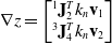 \begin{equation}\nabla{z} =\left[\begin{matrix}{}^1\mathbf{J}_2^Tk_n\mathbf{v}_1 \\{}^3\mathbf{J}_4^Tk_n \mathbf{v}_2\end{matrix}\right]\end{equation}
where $k_n=10$
and
$k_n=10$
and $k_w=0.001$
. The angular velocities
$k_w=0.001$
. The angular velocities ${}^1\omega_0$
and
${}^1\omega_0$
and ${}^3\omega_0$
are read directly from the IMUs.
${}^3\omega_0$
are read directly from the IMUs.
5. Other cases considered
This section presents other cases of bipedal walking that can result in different walking scenarios, given the same robot as in Fig. 1 but using a different control approach.
5.1. Absolute foot movement
The case of absolute foot movement control is where a foot movement is based w.r.t. a hip frame. Using the bipedal robot in Fig. 1, this means that frame {2} moves w.r.t. frame {1} and frame {4} moves w.r.t. frame {3}. In this case, the corresponding absolute Jacobians (as shown above and we state here again for clarity) for leg A is $\mathbf{J}_A = {}^1\mathbf{J}_2\in\mathbb{R}^{3 \times 3}$
and for leg B is
$\mathbf{J}_A = {}^1\mathbf{J}_2\in\mathbb{R}^{3 \times 3}$
and for leg B is $\mathbf{J}_B = {}^3\mathbf{J}_4\in\mathbb{R}^{3 \times 3}$
. In this case, each leg is controlled individually, thus the total torques supplied to the joints will be different from (6), that is,
$\mathbf{J}_B = {}^3\mathbf{J}_4\in\mathbb{R}^{3 \times 3}$
. In this case, each leg is controlled individually, thus the total torques supplied to the joints will be different from (6), that is,
 \begin{equation}\boldsymbol{\tau}_T=\left[\begin{matrix}\boldsymbol{\tau}_A\\\boldsymbol{\tau}_B\end{matrix}\right]=\left[\begin{matrix}\mathbf{J}_A^T{\ddot{\textbf{x}}}_A\\\mathbf{J}_B^T{\ddot{\textbf{x}}}_B\end{matrix}\right]+\left[\begin{matrix}\mathbf{g}_A\\\mathbf{g}_B\end{matrix}\right]\end{equation}
where ${\ddot{\textbf{x}}}_A\in\mathbb{R}^3$
is the
${\ddot{\textbf{x}}}_A\in\mathbb{R}^3$
is the ${\ddot{\textbf{x}}}_B\in\mathbb{R}^3$
. And because each leg moves in the full-position space, the absolute Jacobians
${\ddot{\textbf{x}}}_B\in\mathbb{R}^3$
. And because each leg moves in the full-position space, the absolute Jacobians $\mathbf{J}_A$
and
$\mathbf{J}_A$
and $\mathbf{J}_B$
are not redundant w.r.t.
$\mathbf{J}_B$
are not redundant w.r.t. ${\ddot{\textbf{x}}}_A$
and
${\ddot{\textbf{x}}}_A$
and ${\ddot{\textbf{x}}}_B$
, respectively. That is, all the DOFs of the each Jacobian is utilized to control the absolute foot movement and there is no DOF left to be used for balancing against gravity. Whereas, if relative feet movement is used, (6) will apply where
${\ddot{\textbf{x}}}_B$
, respectively. That is, all the DOFs of the each Jacobian is utilized to control the absolute foot movement and there is no DOF left to be used for balancing against gravity. Whereas, if relative feet movement is used, (6) will apply where $\mathbf{J}_R\in\mathbb{R}^{3 \times 6}$
is redundant w.r.t.
$\mathbf{J}_R\in\mathbb{R}^{3 \times 6}$
is redundant w.r.t. ${\ddot{\textbf{x}}}_R\in\mathbb{R}^3$
. In this case, there will be extra DOFs to be used to balance against gravity.
${\ddot{\textbf{x}}}_R\in\mathbb{R}^3$
. In this case, there will be extra DOFs to be used to balance against gravity.
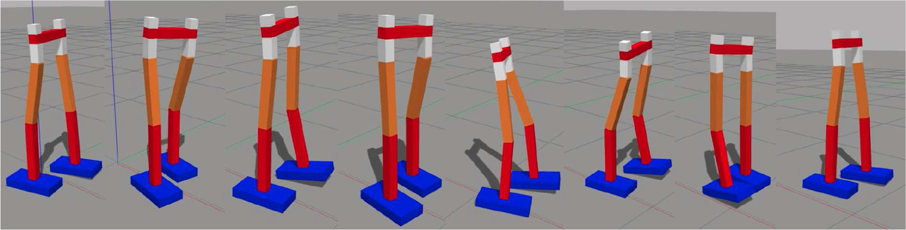
Figure 2. Snapshots of the bipedal robot during the simulation experiment in Gazebo.
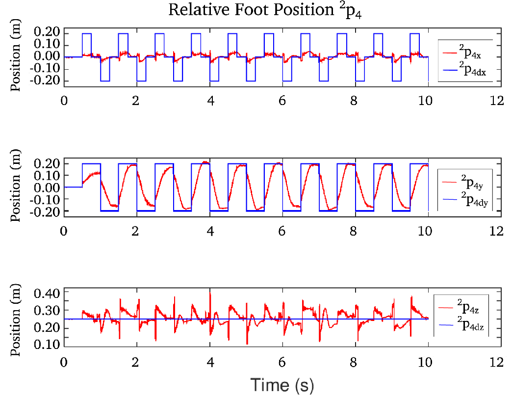
Figure 3. The relative feet position ${}^2\mathbf{p}_4$
plotted against the desired relative position
${}^2\mathbf{p}_4$
plotted against the desired relative position ${}^2\mathbf{p}_{4d}$
.
${}^2\mathbf{p}_{4d}$
.
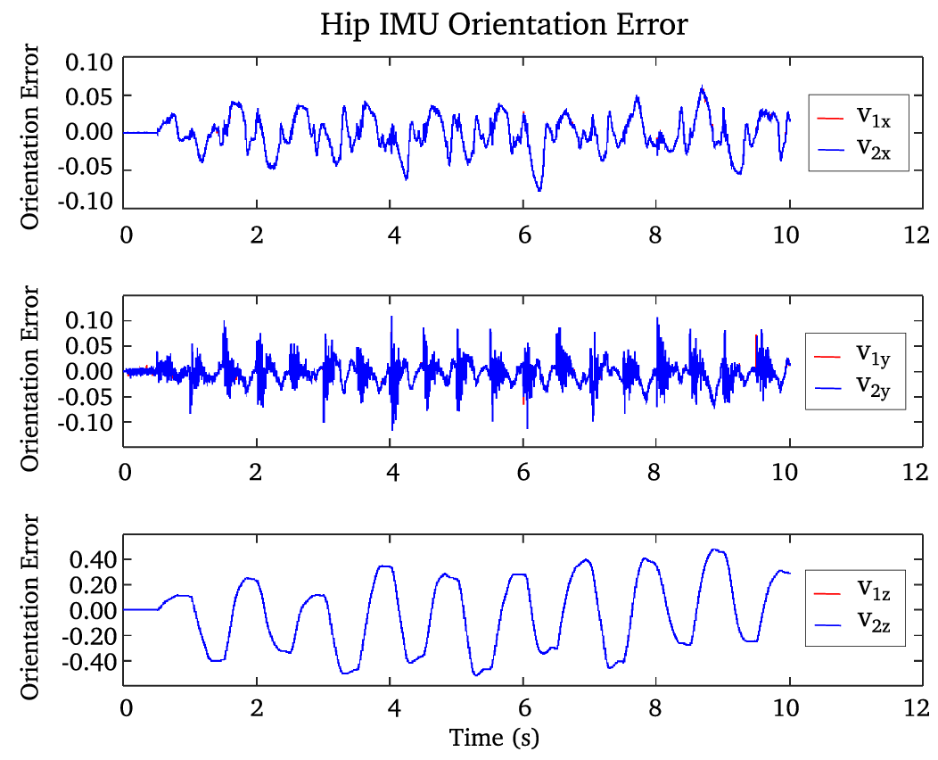
Figure 4. Orientation error of the hip link w.r.t. the world coordinate, based on the feedback of the two IMUs placed at the link ends.
5.2. Relative feet movement with absolute position control
Relative foot movement with balancing against gravity indeed can perform a walking task for a bipedal robot without falling. But to give it a direction of motion w.r.t. the world frame, we would need to specify this additional task to the control equation. In order to achieve this, we modify (6) to become [Reference Jamisola and Roberts8,Reference Jamisola, Chang and Lee55],
 \begin{equation}\boldsymbol{\tau}_T =\mathbf{J}_R^T {\ddot{\textbf{x}}}_R+(\mathbf{I} - \mathbf{J}_R^T \mathbf{J}_R^{+T})\mathbf{J}_O^T\left[\begin{matrix}{}^1\dot{\omega}_0\\{}^3\dot{\omega}_0\end{matrix}\right]+(\mathbf{I} - \mathbf{J}_R^T \mathbf{J}_R^{+T})(\mathbf{I} - \mathbf{J}_O^T \mathbf{J}_O^{+T})\left[\begin{matrix}{}^0\mathbf{J}_2 & \mathbf{0}\end{matrix}\right]^T{}^0{\ddot{\textbf{x}}}_2+\mathbf{g}_T\end{equation}
where $\mathbf{J}_O =[\mathbf{J}_A\;\mathbf{0};\mathbf{0}\;\mathbf{J}_B]$
;
$\mathbf{J}_O =[\mathbf{J}_A\;\mathbf{0};\mathbf{0}\;\mathbf{J}_B]$
; ${}^1\dot{\omega}_0,{}^3\dot{\omega}_0$
are the rotational acceleration of the world frame w.r.t. frame {1} and frame {3}, respectively;
${}^1\dot{\omega}_0,{}^3\dot{\omega}_0$
are the rotational acceleration of the world frame w.r.t. frame {1} and frame {3}, respectively; ${}^0\mathbf{J}_2 = {}^0\mathbf{R}_1 {}^1\mathbf{J}_2$
and
${}^0\mathbf{J}_2 = {}^0\mathbf{R}_1 {}^1\mathbf{J}_2$
and ${}^0\ddot{\mathbf{x}}_2 = {}^0\mathbf{R}_1{}^1\ddot{\mathbf{x}}_2 = [{}^0\ddot{x}_2,{}^0\ddot{y}_2,0]^T$
. Counting the DOF needed for the allocated tasks, there are 3-DOFs for
${}^0\ddot{\mathbf{x}}_2 = {}^0\mathbf{R}_1{}^1\ddot{\mathbf{x}}_2 = [{}^0\ddot{x}_2,{}^0\ddot{y}_2,0]^T$
. Counting the DOF needed for the allocated tasks, there are 3-DOFs for $\ddot{\mathbf{x}}_R$
, 2-DOFs for
$\ddot{\mathbf{x}}_R$
, 2-DOFs for ${}^1\ddot{\mathbf{x}}_2$
, and the remaining 1-DOF for balancing against gravity. However, because balancing has higher priority than
${}^1\ddot{\mathbf{x}}_2$
, and the remaining 1-DOF for balancing against gravity. However, because balancing has higher priority than ${}^1\ddot{\mathbf{x}}_2$
, it can be possible that once
${}^1\ddot{\mathbf{x}}_2$
, it can be possible that once $\ddot{\mathbf{x}}_R$
is performed, all the remaining 3-DOFs will be allocated for balancing before
$\ddot{\mathbf{x}}_R$
is performed, all the remaining 3-DOFs will be allocated for balancing before ${}^1\ddot{\mathbf{x}}_2$
is performed.
${}^1\ddot{\mathbf{x}}_2$
is performed.
6. Results and discussion
Gazebo simulation ran for 40 s, where the alternate foot placement changes at every half a second. The snapshots of the bipedal robot during the simulation are shown in Fig. 2. The relative feet position, ${}^2\mathbf{p}_4$
, is plotted against its desired value and is shown in Fig. 3. The null-space posture error as the bipedal robot tries to balance against gravity is shown in Fig. 4.
${}^2\mathbf{p}_4$
, is plotted against its desired value and is shown in Fig. 3. The null-space posture error as the bipedal robot tries to balance against gravity is shown in Fig. 4.
The value of ${}^2p_{4dy}=\pm0.2m$
is the component of the relative feet position that dictates the forward step. The actual step size
${}^2p_{4dy}=\pm0.2m$
is the component of the relative feet position that dictates the forward step. The actual step size $^2p_{4y}$
achieves close to this value as shown in Fig. 3. The relative distance between the two feet is set at a constant value of
$^2p_{4y}$
achieves close to this value as shown in Fig. 3. The relative distance between the two feet is set at a constant value of ${}^2p_{4dz}=0.25m$
, where the error has a maximum value of around
${}^2p_{4dz}=0.25m$
, where the error has a maximum value of around $0.15m$
. Part of the reason for this large error is because the robot has to position its feet at a relative horizontal distance against each other to counterbalance itself from falling against gravity while walking. Another reason is the fact that this implementation is purely kinematics (with gravity compensation), and thus not as robust as with dynamics modeling/compensation, to focus on the relative Jacobian components responsible for walking and balancing against gravity. The value of
$0.15m$
. Part of the reason for this large error is because the robot has to position its feet at a relative horizontal distance against each other to counterbalance itself from falling against gravity while walking. Another reason is the fact that this implementation is purely kinematics (with gravity compensation), and thus not as robust as with dynamics modeling/compensation, to focus on the relative Jacobian components responsible for walking and balancing against gravity. The value of ${}^2p_{4dx}=\pm0.2m$
is the component that influences the lifting of the foot w.r.t. the other foot (and to the ground). The actual foot lifting was only able to go as high as
${}^2p_{4dx}=\pm0.2m$
is the component that influences the lifting of the foot w.r.t. the other foot (and to the ground). The actual foot lifting was only able to go as high as ${}^2p_{4x}=\pm0.05m$
. In this implementation, the robot had a hard time lifting one foot fully off the ground. And so the robot tends to drag one foot on the ground as it tries to move forward. Hopefully, this current implementation limitation can be addressed in the future with full dynamics modeling and compensation [Reference Jamisola and Dadios56].
${}^2p_{4x}=\pm0.05m$
. In this implementation, the robot had a hard time lifting one foot fully off the ground. And so the robot tends to drag one foot on the ground as it tries to move forward. Hopefully, this current implementation limitation can be addressed in the future with full dynamics modeling and compensation [Reference Jamisola and Dadios56].
The posture error when balancing against gravity is shown in Fig. 4. To be able to balance against gravity without falling, the bipedal robot must maintain this error within certain limits. However, these limits vary and are dependent on the posture of the legs, a similar way to how humans balance against gravity [Reference Meng, Ceccarelli, Yu, Chen and Huang57,Reference Dakin and Rosenberg58]. For example, it is dependent on how the legs posture can afford to exert the required joint torques to avoid a fall, for example, the posture of bent knees with hips pushed forward. Another example is a leg posture that counterbalances the force of gravity, for example, hips pushed sideways but one leg is lifted sideways in the opposite direction. As shown in the graph, the biggest error is the components about the $v_{1z}$
and
$v_{1z}$
and $v_{2z}$
which correspond to how much
$v_{2z}$
which correspond to how much $z_1$
- or
$z_1$
- or $z_3$
-axes digress from the vector normal to the ground. These are directly affected by the disturbance due to the alternate lifting of the two feet relative to each other. The null-space controller tries to keep this error to certain limits such that the robot will not fall against gravity. The rest of the other axes are not as affected by this motion of the feet, although, at some point, the direction of forwarding motion slightly moved sideways due to this disturbance.
$z_3$
-axes digress from the vector normal to the ground. These are directly affected by the disturbance due to the alternate lifting of the two feet relative to each other. The null-space controller tries to keep this error to certain limits such that the robot will not fall against gravity. The rest of the other axes are not as affected by this motion of the feet, although, at some point, the direction of forwarding motion slightly moved sideways due to this disturbance.
7. Conclusion
This work has shown that through a judicious choice of reference frames in bipedal walking, given the same physical robot structure, one can have more legs degrees-of-freedom to perform other leg posture controls while walking. The traditional method of control using fixed reference frames unnecessarily constrained the legs DOFs when walking. The use of relative reference frames releases these constraints using a holistic control approach with two components: (1) world space control using the relative motion between the two feet and (2) null-space control using the posture of the legs to balance against gravity. Control using relative reference frames was possible through the use of modular relative Jacobian. The proposed approach showed a drastic reduction in the required number of leg degrees-of-freedom when performing bipedal walking.
Acknowledgment
The authors would like to thank Olebogeng Mbedzi for his contribution in setting up the Gazebo simulation platform.
Competing interests declaration
The authors declare none.


 Open access