

1. Introduction
The well known Russell’s paper “On denoting” Reference Russell[20] is often treated as a cornerstone of analytic philosophy. In opposition to Meinong’s and Frege’s views, Russell Reference Russell[20] developed his own theory of definite descriptions (abbreviated as RDD), later elaborated in Principia Mathematica Reference Whitehead and Russell[24] and in Reference Russell[21]. Since then RDD is commonly seen as a paradigm of philosophical analysis based on the application of logical tools. Russellian analysis is brilliant and, despite of several criticism and shortcomings, his solution was propagated in hundreds of textbooks as the official theory of definite descriptions.
This paper however is not devoted to a discussion of its advantages and drawbacks, of its philosophical or linguistic merits. In what follows we propose a purely proof theoretic treatment of RDD developed in the setting of sequent calculus (SC). This is a continuation of research on the application of proof theoretic tools to different theories of definite descriptions developed in Reference Indrzejczak, Bezhanishvili, D'Agostino, Metcalfe and Studer[5, 7–9]. Such a study is advantageous for the research on definite descriptions and other term-forming operators, as well as for proof theory. On one side, competing theories of definite descriptions may be shown in the new light, and their formal features may offer new arguments for their utility. On the other hand, it seems that the behavior of term-forming operators needs subtle syntactical analysis enriching a toolkit of proof theory.
We briefly characterize RDD as a formal theory in the shape provided by Kalish, Montague, & Mar Reference Kalish, Montague and Mar[13]. Their treatment of RDD was in terms of natural deduction system (which will be referred to as KMM), useful in practice but not satisfying usual proof theoretic requirements, like normalization. More refined proof theoretic study of term-forming operators, in particular of definite descriptions, in the setting of natural deduction was provided by Tennant Reference Tennant[22, Reference Tennant23] and recently by Kürbis Reference Kürbis[14, Reference Kürbis15]. In fact, in the latter case, definite descriptions are treated as binary quantifiers. Our purpose is to show that it is possible to obtain a satisfactory proof theoretic characterization of RDD in terms of SC.
To this aim we introduce three systems: LKID0, LKID1 and LKID2, all being essentially Gentzen’s original system LK with added special axioms or rules for identity and descriptions, and all equivalent to KMM. LKID0 has an auxiliary character and is introduced only for easier comparison with KMM. LKID1 provides a more refined version which admits, after small refinements, a constructive proof of cut elimination. However, these small refinements make one of the rules for identity not analytic and as a result the subformula property fails. This is connected with the fact that rules for introduction of descriptions treat them as arguments of identities and this may be in conflict with the general rule for introducing identity. The main result of this paper is to show that a more subtle analysis of identities, and atomic formulae in general, can lead to substantial improvement. It is obtained in LKID2 where a richer collection of rules is introduced which are specific for distinct kinds of atomic formulae. As a result for LKID2 we obtain not only constructive proof of cut elimination but also the subformula property.
2. Preliminaries
2.1. Language
We will be using a standard first-order predicate language with quantifiers
 $\forall , \exists $
, identity predicate
$\forall , \exists $
, identity predicate
 $=$
and iota-operator
$=$
and iota-operator
 $\imath $
forming definite descriptions from formulae of the language. In accordance with Gentzen’s custom we divide individual variables into bound
$\imath $
forming definite descriptions from formulae of the language. In accordance with Gentzen’s custom we divide individual variables into bound
 $VAR = \{x,y,z, \ldots \}$
and free variables (parameters)
$VAR = \{x,y,z, \ldots \}$
and free variables (parameters)
 $PAR = \{a, b, c, \ldots \}$
. It makes easier an elaboration of some technical issues concerning substitution and proof transformations. In the metalanguage
$PAR = \{a, b, c, \ldots \}$
. It makes easier an elaboration of some technical issues concerning substitution and proof transformations. In the metalanguage
 $\varphi , \psi , \chi $
denote any formulae and
$\varphi , \psi , \chi $
denote any formulae and
 $\Gamma , \Delta , \Pi , \Sigma $
their multisets. In particular we use a convention to the effect that
$\Gamma , \Delta , \Pi , \Sigma $
their multisets. In particular we use a convention to the effect that
 $\Gamma _1, \ldots , \Gamma _i$
denote submultisets of
$\Gamma _1, \ldots , \Gamma _i$
denote submultisets of
 $\Gamma $
, whereas, e.g.,
$\Gamma $
, whereas, e.g.,
 $\Gamma _{1,2}$
denote multiset union of
$\Gamma _{1,2}$
denote multiset union of
 $\Gamma _1$
and
$\Gamma _1$
and
 $\Gamma _2$
. It facilitates representation of proof schemata involving many-premiss rules.
$\Gamma _2$
. It facilitates representation of proof schemata involving many-premiss rules.
The definition of a term and formula is standard, by simultaneous recursion on both categories. In the presented systems the only terms are variables and definite descriptions since functions may be always represented as descriptions so it is not necessary to consider them separately. As for descriptions, denoting ones are called proper and nondenoting (or not unique) improper. They are written as
 $\imath x\varphi $
where
$\imath x\varphi $
where
 $\varphi $
is a formula in the scope of respective operator. Metavariables
$\varphi $
is a formula in the scope of respective operator. Metavariables
 $t,\, t_1, \ldots $
denote arbitrary terms; moreover, we will use a metavariable d to denote any description if its structure is not essential in the context. We will use also a phrase DD as an abbreviation of “definite description.”
$t,\, t_1, \ldots $
denote arbitrary terms; moreover, we will use a metavariable d to denote any description if its structure is not essential in the context. We will use also a phrase DD as an abbreviation of “definite description.”
 $\varphi [x/t]$
is officially used for the operation of correct substitution of a term t for all occurrences of a variable x in
$\varphi [x/t]$
is officially used for the operation of correct substitution of a term t for all occurrences of a variable x in
 $\varphi $
, and similarly
$\varphi $
, and similarly
 $\Gamma [x/t]$
for a uniform substitution in all formulae in
$\Gamma [x/t]$
for a uniform substitution in all formulae in
 $\Gamma $
. It is always assumed that the substitution thus represented is correct, i.e., if t is a variable or contains variables, they remain free after substitution.
$\Gamma $
. It is always assumed that the substitution thus represented is correct, i.e., if t is a variable or contains variables, they remain free after substitution.
It will be useful to introduce several distinctions concerning formulae which are usually called atomic or elementary. We will keep the latter name for any formula which consists of a predicate (including =) with its arguments. We will call atomic only those elementary formulae where all arguments are variables. If at least one argument is a DD such a formula is quasi-atomic (q-atomic). So elementary formulae are divided into atomic and q-atomic. Moreover, if the predicate is not an identity, such a formula is proper atomic or proper q-atomic (both are called proper elementary). Quasi-atomic identities will be additionally divided into d-identities (both arguments are descriptions) and mixed identities with one argument a parameter and one a DD. Briefly:
(a) elementary formulae are either atomic (no DD) or q-atomic (with DD);
(b) formulae in both categories are proper (proper elementary, proper atomic, and proper q-atomic), if their predicate is not an identity;
(c) identities (i.e., non-proper elementary formulae) are either atomic (no DD) or q-atomic, and the latter are either mixed identities (one argument DD) or d-identities (both arguments DD).
A distinction between atomic and q-atomic formula is connected with the complexity of formulae/terms which is defined simultaneously for both categories:
 $c(t) = 0$
, for t being a variable (bound or free),
$c(t) = 0$
, for t being a variable (bound or free),
 $c(\imath x\varphi ) = c(\neg \varphi ) = c(\forall x\varphi )= c(\exists x\varphi ) = c(\varphi )+1$
,
$c(\imath x\varphi ) = c(\neg \varphi ) = c(\forall x\varphi )= c(\exists x\varphi ) = c(\varphi )+1$
,
 $c(\varphi \ast \psi ) = c(\varphi )+c(\psi )+1$
, for
$c(\varphi \ast \psi ) = c(\varphi )+c(\psi )+1$
, for
 $\ast \in \{\wedge , \vee , \rightarrow , \leftrightarrow \}$
,
$\ast \in \{\wedge , \vee , \rightarrow , \leftrightarrow \}$
,
 $c(R^nt_1\ldots t_n) = \sum ^n_{i=1} c(t_i) +1$
,
$c(R^nt_1\ldots t_n) = \sum ^n_{i=1} c(t_i) +1$
,
 $c(t_1=t_2)= c(t_1)+c(t_2)$
.
$c(t_1=t_2)= c(t_1)+c(t_2)$
.
One may easily observe that all atomic formulae have complexity either 1 (proper atomic) or 0 (atomic identity) whereas q-atomic formulae may be more complex than compound formulae. That is an important factor in proving cut elimination. Treating proper elementary formulae as more complex than identities may seem counterintuitive but it is dictated by the requirements of this proof.
2.2. Russellian theory of descriptions
We will focus on proof-theoretic matters, in particular, we show that by means of a well-balanced treatment of identity rules we can obtain a system which satisfies cut-elimination and is analytic. However, before we jump to the proper aim of this research, a brief explanation of what we mean by Russellian definite description theory (RDD) is necessary.
Both Frege and Russell assumed that terms must denote but react in different ways for the failure of denotation (the phenomenon of improper descriptions). Frege considered four different attempts, analyzed by Pelletier & Linsky Reference Pelletier, Linsky, Griffin and Jacquette[18], and at least in his two proposals urged that all descriptions must have designates, even if it will be arbitrary. Incidentally, this last option, often called the chosen object theory, was also formalized by Kalish et al. Reference Kalish, Montague and Mar[13] as a natural deduction system and by Indrzejczak Reference Indrzejczak[7] as a cut-free SC. On the other hand, Russell denied that descriptions are terms and left variables as the only terms of the formal language of mathematics. The other option, namely admitting non-denoting terms, was first proposed by Jaśkowski Reference Jaśkowski[12] and then developed by several researchers under the heading of free logics.
Therefore, the original Russellian treatment of descriptions represents a kind of eliminativist approach. In contrast to Frege’s view, Russell treated descriptions as a kind of incomplete signs and showed how to get rid of them by means of contextual definitions of the form:
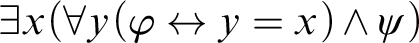
 $$ \begin{align*} \psi[x/\imath y\varphi] \ := \ \exists x(\forall y(\varphi \leftrightarrow y =x )\wedge\psi). \end{align*} $$
The analysis in Reference Russell[20] is brilliant and seems to be commonly accepted; hundreds of textbooks using it as the official theory of descriptions count as good witness of this claim. However, this way of doing things has its own drawbacks connected with scoping difficulties if
 $\psi $
is not elementary. To avoid them Whitehead & Russell Reference Whitehead and Russell[24] introduced additional devices allowing formal control over the scope of description. On the other hand, in Reference Whitehead and Russell[24] one may find several theorems formulated with descriptions occurring in term position. Pelletier & Linsky Reference Pelletier, Linsky, Griffin and Jacquette[18] provide also a list of theorems and rules correct in RDD. Finally in Reference Kalish, Montague and Mar[13] one may find a natural deduction system characterizing RDD which we call KMM. This shows that it is possible to save some features of the Russellian approach to descriptions yet to treat them as genuine terms. In what follows we provide sequent systems which are equivalent to KMM and in this sense provide a proof theoretic formalizations of RDD. What features are central for saving the spirit of RDD, if we do not try to eliminate descriptions from every context but rather to develop a suitable logic of descriptions as terms? In the Russellian approach there seem to be:
$\psi $
is not elementary. To avoid them Whitehead & Russell Reference Whitehead and Russell[24] introduced additional devices allowing formal control over the scope of description. On the other hand, in Reference Whitehead and Russell[24] one may find several theorems formulated with descriptions occurring in term position. Pelletier & Linsky Reference Pelletier, Linsky, Griffin and Jacquette[18] provide also a list of theorems and rules correct in RDD. Finally in Reference Kalish, Montague and Mar[13] one may find a natural deduction system characterizing RDD which we call KMM. This shows that it is possible to save some features of the Russellian approach to descriptions yet to treat them as genuine terms. In what follows we provide sequent systems which are equivalent to KMM and in this sense provide a proof theoretic formalizations of RDD. What features are central for saving the spirit of RDD, if we do not try to eliminate descriptions from every context but rather to develop a suitable logic of descriptions as terms? In the Russellian approach there seem to be:
-
1. fixed evaluation (as false) of all elementary formulae with nondenoting terms;
-
2. quantification rules of universal instantiation UI and existential generalization EG restricted to variables;
-
3. identity with reflexivity restricted to variables;
-
4. taking object language counterpart of Russellian definition as an axiom characterizing descriptions (we will call it R):
 $$ \begin{align*} \text{R} \ \psi[x/\imath y\varphi] \leftrightarrow \exists x(\forall y(\varphi \leftrightarrow y =x )\wedge\psi), \end{align*} $$
where
 $\psi $
must be elementary. This restriction is important since unrestricted version can lead to contradiction. If we use tautology for
$\psi $
must be elementary. This restriction is important since unrestricted version can lead to contradiction. If we use tautology for
 $\psi $
and contradiction for
$\psi $
and contradiction for
 $\varphi $
in the schema we get troubles. For example:
$\varphi $
in the schema we get troubles. For example:
 $$ \begin{align*} A(\imath y(By\wedge\neg By))\rightarrow A(\imath y(By\wedge\neg By)) \leftrightarrow \exists x(\forall y(By\wedge\neg By \leftrightarrow y = x)\wedge (Ax\rightarrow Ax)) \end{align*} $$
leads to
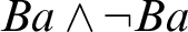 $Ba\wedge \neg Ba$
.
$Ba\wedge \neg Ba$
.
The first three features concern the background logic whereas the last one is a specific characterization of descriptions. In fact the most important feature is 1; 2 and 3 are its consequences. In 2 we mean that when a universal quantifier is eliminated we cannot unrestrictedly substitute quantified variable with an arbitrary term satisfying the conditions of proper substitution. In case of nondenoting term we can deduce a formula which is false because of 1. Therefore the rule of universal elimination (or existential generalization) must be restricted to such terms of which it was earlier established that they denote. In KMM both rules are simply restricted to variables as instantiated terms and it is assumed that all variables are denoting. Similarly in p. 3 if t is nondenoting, then even
 $t=t$
is false according to 1. Therefore reflexivity must be restricted to denoting terms. Summing up these three features call for a logic which is currently identified as a kind of negative free logic.
$t=t$
is false according to 1. Therefore reflexivity must be restricted to denoting terms. Summing up these three features call for a logic which is currently identified as a kind of negative free logic.
4 is also sensitive to the choice of background logic. R cannot be just added to FOL with unrestricted UI and EG, since it leads to inconsistency. Restricting logic according to the points 1–3 makes possible to use R without problems. However, the fact that underlying logic is a negative free logic allows us to replace R with another formula which is easier to deal with. It is the well known Lambert axiom:
 $$ \begin{align*} LA \ \ \forall x(x=\imath y\varphi \leftrightarrow \forall y(\varphi\leftrightarrow y=x)). \end{align*} $$
2.3. The system of Kalish, Montague and Mar
In focusing on these four features we follow Chapter VIII of Reference Kalish, Montague and Mar[13]. They present their version of RDD in the setting of natural deduction (ND). Leaving aside the idiosyncrasies of their ND system, called KMM in what follows, we mention that it is based on classical FOL in the language where terms consist only of variables and individual constants. It is well known that functional terms can be presented by means of descriptions so it is a reasonable choice. In our version we get rid of individual constants as well, since they can be also reduced to definite descriptions in the similar way. On the other hand, we follow a Gentzen’s custom of making a graphic distinction between bound and free variables (parameters) which is absent in KMM.
So what is the system we call KMM? To obtain an ND-system for RDD, in Reference Kalish, Montague and Mar[13] the basic ND for FOL, with UI and EG restricted to variables, is completed with the following rules:
 $$ \begin{align*} \begin{array}{ll} (ID) & \ \ \varnothing \vdash b=b. \\ (LL) & \ \ t_1=t_2, \varphi[x/t_1] \vdash \varphi[x/t_2]. \\ (DP-1) & \ \ R^n t_1 \ldots t_n \vdash \exists xx=t_1 \wedge\cdots\wedge \exists xx=t_n. \\ (DP-2) & \ \ t_1=t_2 \vdash\exists xx=t_1. \\ (RD) & \ \ \varnothing\vdash\forall x(x=\imath y\varphi \leftrightarrow \forall y(\varphi\leftrightarrow y=x)). \end{array} \end{align*} $$
The restricted form of
 $(ID)$
expresses the fact that variables always denote. In RDD
$(ID)$
expresses the fact that variables always denote. In RDD
 $d=d$
does not hold in general; however, it holds
$d=d$
does not hold in general; however, it holds
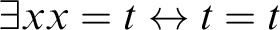 $\exists xx=t\leftrightarrow t=t$
.
$\exists xx=t\leftrightarrow t=t$
.
 $(LL)$
is for the Leibniz’ law. Both denotation principles
$(LL)$
is for the Leibniz’ law. Both denotation principles
 $(DP$
-
$(DP$
-
 $1), (DP$
-
$1), (DP$
-
 $2)$
are necessary to satisfy Russellian treatment of elementary formulae with nondenoting terms.
$2)$
are necessary to satisfy Russellian treatment of elementary formulae with nondenoting terms.
 $(RD)$
is just the Lambert axiom taken as zero-premiss rule. Although in general it is weaker than R, in the presence of denotation principles it is equivalent to R. We sketch a proof.
$(RD)$
is just the Lambert axiom taken as zero-premiss rule. Although in general it is weaker than R, in the presence of denotation principles it is equivalent to R. We sketch a proof.
Lemma 2.1. R and (RD) are equivalent in KMM.
Proof. To prove R assume first
 $\exists x(\forall y(\varphi \leftrightarrow y=x)\wedge \psi )$
. Using an arbitrary fresh parameter a we obtain
$\exists x(\forall y(\varphi \leftrightarrow y=x)\wedge \psi )$
. Using an arbitrary fresh parameter a we obtain
 $\forall y(\varphi \leftrightarrow y = a)$
and
$\forall y(\varphi \leftrightarrow y = a)$
and
 $\psi [x/a]$
. From
$\psi [x/a]$
. From
 $(RD)$
by universal instantiation we obtain
$(RD)$
by universal instantiation we obtain
 $a=\imath y\varphi \leftrightarrow \forall y(\varphi \leftrightarrow y = a)$
which, by the former formula, yields
$a=\imath y\varphi \leftrightarrow \forall y(\varphi \leftrightarrow y = a)$
which, by the former formula, yields
 $a=\imath y\varphi $
. By
$a=\imath y\varphi $
. By
 $(LL)$
on
$(LL)$
on
 $\psi [x/a]$
we obtain
$\psi [x/a]$
we obtain
 $\psi [x/\imath y\varphi ]$
. Since a was fresh in the reasoning, this formula follows from
$\psi [x/\imath y\varphi ]$
. Since a was fresh in the reasoning, this formula follows from
 $\exists x(\forall y(\varphi \leftrightarrow y=x)\wedge \psi )$
.
$\exists x(\forall y(\varphi \leftrightarrow y=x)\wedge \psi )$
.
If we assume
 $\psi [x/\imath y\varphi ]$
, then by
$\psi [x/\imath y\varphi ]$
, then by
 $(DP$
-
$(DP$
-
 $1)$
, and possibly conjunction elimination, (or
$1)$
, and possibly conjunction elimination, (or
 $(DP$
-
$(DP$
-
 $2)$
) we get
$2)$
) we get
 $\exists xx=\imath y\varphi $
, since
$\exists xx=\imath y\varphi $
, since
 $\psi $
is elementary. Again using fresh a we obtain
$\psi $
is elementary. Again using fresh a we obtain
 $a=\imath y\varphi $
and then by
$a=\imath y\varphi $
and then by
 $(LL)$
,
$(LL)$
,
 $\psi [x/a]$
. Furthermore
$\psi [x/a]$
. Furthermore
 $a=\imath y\varphi \leftrightarrow \forall y(\varphi \leftrightarrow y = a)$
by universal instantiation from
$a=\imath y\varphi \leftrightarrow \forall y(\varphi \leftrightarrow y = a)$
by universal instantiation from
 $(RD)$
. These two formulae by detachment yield
$(RD)$
. These two formulae by detachment yield
 $\forall y(\varphi \leftrightarrow y = a)$
. This, together with
$\forall y(\varphi \leftrightarrow y = a)$
. This, together with
 $\psi [x/a]$
, yields by EG
$\psi [x/a]$
, yields by EG
 $\exists x(\forall y(\varphi \leftrightarrow y = x)\wedge \psi )$
.
$\exists x(\forall y(\varphi \leftrightarrow y = x)\wedge \psi )$
.
To prove
 $(RD)$
assume first for some arbitrary a,
$(RD)$
assume first for some arbitrary a,
 $a=\imath y\varphi $
and using
$a=\imath y\varphi $
and using
 $a=x$
as our elementary
$a=x$
as our elementary
 $\psi $
in R we obtain
$\psi $
in R we obtain
 $\exists x(\forall y(\varphi \leftrightarrow y = x)\wedge a=x)$
which by instantiation yields
$\exists x(\forall y(\varphi \leftrightarrow y = x)\wedge a=x)$
which by instantiation yields
 $\forall y(\varphi \leftrightarrow y =b )$
and
$\forall y(\varphi \leftrightarrow y =b )$
and
 $a=b$
. By
$a=b$
. By
 $(LL)$
we obtain
$(LL)$
we obtain
 $\forall y(\varphi \leftrightarrow y = a)$
. For the converse, if we assume the latter and add
$\forall y(\varphi \leftrightarrow y = a)$
. For the converse, if we assume the latter and add
 $a=a$
we can deduce
$a=a$
we can deduce
 $\exists x(\forall y(\varphi \leftrightarrow y=x)\wedge a=x)$
by existential generalization. This by R yields
$\exists x(\forall y(\varphi \leftrightarrow y=x)\wedge a=x)$
by existential generalization. This by R yields
 $a=\imath y\varphi $
. Combining both implications and applying universal generalization (since a was arbitrary) we obtain
$a=\imath y\varphi $
. Combining both implications and applying universal generalization (since a was arbitrary) we obtain
 $(RD)$
.□
$(RD)$
.□
It should be noted that denotation principles were required in proving one direction of R by means of
 $(RD)$
. So in positive free logics the latter principle is essentially weaker.
$(RD)$
. So in positive free logics the latter principle is essentially weaker.
One may also easily show that the restricted rules of universal instantiation and existential generalization are sufficient to provide instantiation also for descriptions, if they are proper. Namely, we can prove that these two rules are derivable in KMM:
 $$ \begin{align*} &\forall x\varphi, \exists xx=d\vdash \varphi[x/d],\\ &\varphi[x/d], \exists xx=d\vdash \exists x\varphi. \end{align*} $$
For the first if we instantiate the second premiss with fresh a we obtain
 $a=d$
and may apply universal instantiation obtaining
$a=d$
and may apply universal instantiation obtaining
 $\varphi [x/a]$
. By
$\varphi [x/a]$
. By
 $(LL)$
we obtain
$(LL)$
we obtain
 $\varphi [x/d]$
. The second proof is similar.
$\varphi [x/d]$
. The second proof is similar.
It may be instructive to provide a list of some theorems of RDD taken from Principia Mathematica (PM) or KMM; in the brackets there is a number of suitable theorems from PM (all beginning with 14.) or KMM (beginning with 5). Many of them are equivalences or implications having
 $E\imath x\varphi $
(Principia Mathematica) or
$E\imath x\varphi $
(Principia Mathematica) or
 $\exists yy=\imath x\varphi $
(KMM) as an antecedent. E in free logics is often used as an unary predicate and may be defined as
$\exists yy=\imath x\varphi $
(KMM) as an antecedent. E in free logics is often used as an unary predicate and may be defined as
 $Et := \exists yy=t$
. In Principia Mathematica E is used only with descriptions and they are defined jointly in the following way:
$Et := \exists yy=t$
. In Principia Mathematica E is used only with descriptions and they are defined jointly in the following way:
 $E\imath x\varphi := \exists y\forall x(\varphi \leftrightarrow x=y)$
. However, it can be proved that in RDD
$E\imath x\varphi := \exists y\forall x(\varphi \leftrightarrow x=y)$
. However, it can be proved that in RDD
 $\exists yy=\imath x\varphi $
is equivalent to
$\exists yy=\imath x\varphi $
is equivalent to
 $\exists y\forall x(\varphi \leftrightarrow x=y)$
. So we are justified in treating them uniformly and we use
$\exists y\forall x(\varphi \leftrightarrow x=y)$
. So we are justified in treating them uniformly and we use
 $\sigma $
as a fixed symbol for such antecedent.
$\sigma $
as a fixed symbol for such antecedent.
 $$ \begin{align*} &\sigma \leftrightarrow \varphi\ [x/\imath x\varphi]\ [14.22, 502]\\ &\sigma \leftrightarrow \imath x\varphi=\imath x\varphi\ [14.28, 501]\\ &\sigma \leftrightarrow \exists y \imath x\varphi=y\ [14.204]\\ &\sigma \leftrightarrow \exists y\forall x(\varphi\leftrightarrow x=y)\ [14.11, 500]\\ &\sigma \leftrightarrow \exists x\varphi\wedge \forall xy(\varphi \wedge \varphi\ [x/y]\rightarrow x=y)\ [14.203]\\ &\sigma \rightarrow \exists x\varphi\ [14.201]\\ &\sigma \rightarrow \imath x\varphi=\imath y\varphi\ [x/y]\ [505]\\ &\sigma \rightarrow \forall xy(\varphi \wedge \varphi\ [x/y]\rightarrow x=y)\ [14.12]\\ &\sigma \rightarrow (\forall y\psi\rightarrow \psi\ [y/\imath x\varphi])\ [14.18, 527]\\ &\sigma \rightarrow \imath x(x =\imath x\varphi)=\imath x\varphi\ [513]\\ &\sigma \rightarrow \forall x(\varphi\leftrightarrow x=\imath x\varphi)\ [14.241, 506]\\ &\sigma \rightarrow (\forall x(\varphi\rightarrow\psi)\leftrightarrow \psi\ [x/\imath x\varphi])\ [14.25]\\ &\sigma \rightarrow (\exists x(\varphi\wedge\psi)\leftrightarrow \psi\ [x/\imath x\varphi])\ [14.26]\\ &\sigma \rightarrow (\forall x(\varphi\leftrightarrow\psi)\leftrightarrow \imath x\varphi = \imath x \psi)\ [14.27, 504] \end{align*} $$
Theorem 14.28 shows that d-identity is not reflexive in general; on the other hand, symmetry and transitivity holds unconditionally for identities with any terms (Theorems 14.13, 14.131, 14.14, 14.142, and 14.144 in PM).
Some other theorems of interest:
 $$ \begin{align*} &\imath x(x=y)=y\ [14.2]\\ &\neg\varphi\ [x/\imath x\neg\varphi]\ [516]\\ &\psi\ [x/\imath x\varphi] \leftrightarrow \psi\ [x/\imath y \varphi\ [x/y]])\ [14.272,\ \text{KMM p.} 407,\ \text{Ex.} 19]\\ &\forall z(z=\imath x\varphi \leftrightarrow z=\imath y\varphi\ [x/y])\ [\text{KMM p.}\ 407,\ \text{Ex.} 19]\\ & \imath x\varphi = \imath x \psi \rightarrow \forall x(\varphi\leftrightarrow\psi)\ [508]\\ &E\imath x(\varphi\wedge\psi) \leftrightarrow \varphi\ [x/\imath x (\varphi\wedge\psi)]\ [14.23]\\ &\forall x(\varphi\leftrightarrow\psi)\rightarrow (E\imath x\varphi \leftrightarrow E\imath x \psi)\ [14.271]\\ &\forall x(\varphi\leftrightarrow\psi)\rightarrow (\chi\ [x/\imath x\varphi] \leftrightarrow \chi\ [x/\imath x \psi])\ [14.272,\ \text{KMM p.} 407,\ \text{Ex.} 19]\\ &\forall x(\varphi\leftrightarrow\psi)\rightarrow \forall y(y=\imath x\varphi \leftrightarrow y=\imath x \psi)\ [\text{KMM p.} 407,\ \text{Ex.} 19]\\ &\forall x(\varphi\leftrightarrow x=y)\rightarrow (\psi\ [x/\imath x\varphi] \leftrightarrow \psi\ [x/y])\ [14.242]\\ &\forall x(\varphi\leftrightarrow x=y)\leftrightarrow \imath x\varphi =y\ [14.202, 510]\\ &\imath x\varphi = y\rightarrow (\chi\ [x/\imath x\varphi] \leftrightarrow \chi\ [x/y])\ [14.15]\\ &\imath x\varphi = \imath x\psi\rightarrow (\chi\ [x/\imath x\varphi] \leftrightarrow \chi\ [x/\imath x \psi])\ [14.16]\\ &y=\imath x\varphi \wedge y= \imath x\psi\rightarrow \imath x\varphi=\imath x \psi\ [14.145]\\ &\psi\ [x/\imath x\varphi] \wedge \psi\ [x/\imath x\neg\varphi]\rightarrow \neg\psi\ [x/\imath x \psi]\ [522]\\ &\psi\ [x/\imath x\varphi] \wedge \varphi\ [x/\imath x\psi]\rightarrow \imath x\varphi=\imath x \psi\ [523]\\ &\psi\ [x/\imath x\varphi] \leftrightarrow \exists x(x=\imath x\varphi\wedge \psi)\ [14.205]\\ &\neg \exists yy=\imath x\varphi \wedge \neg \exists yy=\imath x\psi\rightarrow \forall y(y=\imath x\varphi \leftrightarrow y= \imath x \psi)\ [511]\\ &\neg \psi\ [y/\imath x\varphi] \leftrightarrow \exists y(\forall x(\varphi\leftrightarrow x=y) \wedge \neg \psi)\vee \neg E\imath x\varphi\ [517] \end{align*} $$
Note that the converse of 508 does not hold which makes extensionality problematic. But 504 (14.27) is its weakened conditional counterpart which for some applications may be sufficient. Theorem 517 is a negated counterpart of R.
2.4. The basic sequent calculus LK
Before we undertake an investigation on SC characterization of KMM let us consider in separation the core system for identity-free and description-free language. While in all presented systems for KMM the rules for identity and definite descriptions will be strongly interrelated and committed to changes, this basis is fixed and provides SC for pure (i.e., with variables as the only terms) classical FOL. It consists of the following structural and logical rules:
 $$ \begin{align*} &(AX) \ \varphi \Rightarrow \varphi \hspace{9.51pc} (Cut) \ \frac{{\Gamma \!\!\Rightarrow \Delta, \varphi \hspace{.5cm} \varphi , \Pi \!\!\Rightarrow \Sigma }}{{\Gamma, \Pi \!\!\Rightarrow \Delta, \Sigma }}\\ &(W\!\!\Rightarrow) \ \frac{{\Gamma \!\!\Rightarrow \Delta}}{{\varphi, \Gamma \!\!\Rightarrow \Delta}} \hspace{8.3pc} (\Rightarrow\!\!W) \ \frac{{\Gamma \!\!\Rightarrow \Delta}}{{\Gamma \!\!\Rightarrow \Delta, \varphi}}\\ &(C\!\!\Rightarrow) \ \frac{{\varphi , \varphi , \Gamma \!\!\Rightarrow \Delta}}{{\varphi, \Gamma \!\!\Rightarrow \Delta}} \hspace{7.7pc} (\Rightarrow\!\!C) \ \frac{{\Gamma \!\!\Rightarrow \Delta, \varphi , \varphi }}{{\Gamma \!\!\Rightarrow \Delta, \varphi}}\\ &(\neg\!\!\Rightarrow) \ \frac{{\Gamma \!\!\Rightarrow \Delta, \varphi}}{{\neg\varphi, \Gamma \!\!\Rightarrow \Delta}} \hspace{8.15pc} (\Rightarrow\!\!\neg) \ \frac{{\varphi, \Gamma \!\!\Rightarrow \Delta}}{{\Gamma \!\!\Rightarrow \Delta, \neg\varphi}}\\ &(\wedge\!\!\Rightarrow) \ \frac{{\varphi, \psi, \Gamma \!\!\Rightarrow \Delta}}{{\varphi\!\wedge\!\psi, \Gamma \!\!\Rightarrow \Delta}} \hspace{7.5pc} (\Rightarrow\!\!\wedge) \ \frac{{\Gamma \!\!\Rightarrow \Delta, \varphi \hspace{.5cm} \Pi \!\!\Rightarrow \Sigma , \psi}}{{\Gamma, \Pi \!\!\Rightarrow \Delta, \Sigma, \varphi\!\wedge\!\psi}}\\ &(\vee\!\!\Rightarrow) \ \frac{{\varphi, \Gamma \!\!\Rightarrow \Delta \hspace{.5cm} \psi, \Pi \!\!\Rightarrow \Sigma }}{{\varphi\!\vee\!\psi, \Gamma, \Pi \!\!\Rightarrow \Delta, \Sigma }} \hspace{4.45pc} (\Rightarrow\!\!\vee) \ \frac{{\Gamma \!\!\Rightarrow \Delta, \varphi, \psi}}{{\Gamma \!\!\Rightarrow \Delta, \varphi\!\vee\!\psi}}\\ &(\rightarrow\Rightarrow) \ \frac{{\Gamma \!\!\Rightarrow \Delta, \varphi \hspace{.5cm} \psi, \Pi \!\!\Rightarrow \Sigma }}{{\varphi\!\rightarrow\!\psi, \Gamma, \Pi \!\!\Rightarrow \Delta, \Sigma }} \hspace{4.17pc} (\Rightarrow\rightarrow) \ \frac{{\varphi, \Gamma \!\!\Rightarrow \Delta, \psi}}{{\Gamma \!\!\Rightarrow \Delta, \varphi\!\rightarrow\!\psi}}\\ &(\leftrightarrow\Rightarrow) \ \frac{{\Gamma \!\!\Rightarrow \Delta, \varphi, \psi \hspace{.5cm} \varphi, \psi, \Pi \!\!\Rightarrow \Sigma }}{{\varphi\!\leftrightarrow\!\psi, \Gamma, \Pi \!\!\Rightarrow \Delta, \Sigma }} \qquad\quad (\Rightarrow\leftrightarrow) \ \frac{{\varphi, \Gamma \!\!\Rightarrow \Delta, \psi \hspace{.5cm} \psi, \Pi \Rightarrow \Sigma, \varphi}}{{\Gamma, \Pi \!\!\Rightarrow \Delta, \Sigma, \varphi\!\leftrightarrow\!\psi}}\\ &(\forall \!\!\Rightarrow) \ \frac{{ \varphi[x/b], \Gamma \!\!\Rightarrow \Delta }}{{\forall x\varphi, \Gamma \!\!\Rightarrow \Delta }}\hspace{6.3pc} (\Rightarrow\!\!\forall) \ \frac{{\Gamma \!\!\Rightarrow \Delta, \varphi[x/a] }}{{\Gamma \!\!\Rightarrow \Delta, \forall x\varphi}}\\ &(\exists\!\!\Rightarrow) \ \frac{{\varphi[x/a], \Gamma \!\!\Rightarrow \Delta }}{{\exists x\varphi, \Gamma \!\!\Rightarrow \Delta }} \hspace{6.3pc} (\Rightarrow\!\!\exists ) \ \frac{{\Gamma \!\!\Rightarrow \Delta, \varphi[x/b] }}{{\Gamma \!\!\Rightarrow \Delta, \exists x\varphi }} \end{align*} $$
where a (called the eigenvariable after Gentzen) is not in
 $\Gamma , \Delta $
and
$\Gamma , \Delta $
and
 $\varphi $
, whereas b is any parameter. This convention will be applied throughout.
$\varphi $
, whereas b is any parameter. This convention will be applied throughout.
The definition of proofs is standard; they are built as trees with the root labeled with a proven sequent, leaves with axioms and remaining nodes regulated by the application of rules. The height of a proof of a given sequent is the length of maximal branches of its proof. We keep also standard terminology with respect to components of rules; in particular displayed formulae in the schemata of rules are active (principal in the conclusion and side-formulae in the premisses) and remaining ones are parametric and together make a context.
This system provides an adequate formalization of pure FOL and we will call it LK, since it is essentially Gentzen’s LK with small differences: (1) Sequents of the form
 $\Gamma \Rightarrow \Delta $
are built from finite multisets not sequences to avoid inessential complications. (2) We also prefer to present all two-premiss rules in the multiplicative (or with independent contexts) version. (3) We display additionally rules for equivalence which are not usually formulated but are crucial for our analysis of descriptions. (4) Terms in quantifier rules are restricted to variables. The last point is not really a restriction in the case of pure FOL. Of course there is no problem to include individual constants as in the original KMM; it is sufficient to replace b with t in
$\Gamma \Rightarrow \Delta $
are built from finite multisets not sequences to avoid inessential complications. (2) We also prefer to present all two-premiss rules in the multiplicative (or with independent contexts) version. (3) We display additionally rules for equivalence which are not usually formulated but are crucial for our analysis of descriptions. (4) Terms in quantifier rules are restricted to variables. The last point is not really a restriction in the case of pure FOL. Of course there is no problem to include individual constants as in the original KMM; it is sufficient to replace b with t in
 $(\forall \Rightarrow ), (\Rightarrow \exists )$
where t is either a parameter or an individual constant (but not definite description). Thus we take for granted that LK is equivalent to the restricted part of KMM system without identity and descriptions (and individual constants). Before we focus on these additions it is worthwhile to consider the well known properties of LK, since they will be our point of departure in projecting a decent SC for RDD.
$(\forall \Rightarrow ), (\Rightarrow \exists )$
where t is either a parameter or an individual constant (but not definite description). Thus we take for granted that LK is equivalent to the restricted part of KMM system without identity and descriptions (and individual constants). Before we focus on these additions it is worthwhile to consider the well known properties of LK, since they will be our point of departure in projecting a decent SC for RDD.
Theorem 2.2 (Properties of LK)
-
1. If
 $\vdash _k \Gamma \Rightarrow \Delta $
, then
$\vdash _k \Gamma [a/b] \Rightarrow \Delta [a/b]$
, where k is the height of a proof.
$\vdash _k \Gamma \Rightarrow \Delta $
, then
$\vdash _k \Gamma [a/b] \Rightarrow \Delta [a/b]$
, where k is the height of a proof. -
2. If
$\vdash \Gamma \Rightarrow \Delta $
, then
$\vdash \Gamma \Rightarrow \Delta $
is cut-free provable. -
3. If
$\vdash \Gamma \Rightarrow \Delta $
has a cut-free proof, then it is constructed from subformulae of
$\Gamma , \Delta $
.


These are familiar properties of (1) substitution, (2) cut elimination and (3) the subformula property. The last one follows from the second as can be easily checked by the inspection of rules. Substitution is an auxiliary result needed for proving (2); in particular it helps to change all proofs into regular proofs, in the sense that every parameter which is fresh by side condition on the respective rule must be fresh in the entire proof, not only on the branch where the application of this rule takes place. Thus no eigenvariable is used more than once in the whole regular proof which simplifies the cut elimination proof. In what follows we assume that we deal only with such proofs; there is no loss of generality since every proof may be systematically transformed into a regular one by the substitution lemma.
Cut elimination is the crucial point, sufficient, at least for LK and similar variants of SC, for obtaining a proof system which is often said to be analytic. For proving (2) usually combinatorial inductive proofs are provided showing how to systematically reduce the complexity of cut formulae and transform every proof into a cut-free proof. This systematic reduction is based on at least two inductive parameters: the height of the proof tree and the cut-rank which, for our purposes is defined as the complexity of the cut-formula. Accordingly we can call them h- and r-reduction, since the proof proceeds by reducing either the height of one of the premisses (if the cut formula is not principal there) or the complexity of the cut formula (if the cut formula is principal in both premisses). The interplay between these two kinds of reduction is particularly well illustrated by the specific strategy originally introduced for hypersequent calculi by Metcalfe, Olivetti, & Gabbay Reference Metcalfe, Olivetti and Gabbay[16] and later extensively used in this framework but applicable also to standard sequent calculi (see Reference Indrzejczak[10]). We will designate the cut-rank as
 $r\varphi $
and accordingly
$r\varphi $
and accordingly
 $r{\cal D}$
will denote the proof-rank, i.e., the maximal cut-rank in
$r{\cal D}$
will denote the proof-rank, i.e., the maximal cut-rank in
 ${\cal D}$
.
${\cal D}$
.
The cut elimination theorem follows from two lemmata:
Lemma 2.3 (Right reduction)
Let
 ${\cal D}_1 \vdash \Gamma \Rightarrow \Delta , \varphi $
and
${\cal D}_1 \vdash \Gamma \Rightarrow \Delta , \varphi $
and
 ${\cal D}_2 \vdash \varphi ^k, \Pi \Rightarrow \Sigma $
with
${\cal D}_2 \vdash \varphi ^k, \Pi \Rightarrow \Sigma $
with
 $r{\cal D}_1, r{\cal D}_2 < r\varphi $
, and
$r{\cal D}_1, r{\cal D}_2 < r\varphi $
, and
 $\varphi $
principal in
$\varphi $
principal in
 $\Gamma \Rightarrow \Delta , \varphi $
, then we can construct a proof
$\Gamma \Rightarrow \Delta , \varphi $
, then we can construct a proof
 ${\cal D}$
such that
${\cal D}$
such that
 ${\cal D} \vdash \Gamma ^k, \Pi \Rightarrow \Delta ^k, \Sigma $
and
${\cal D} \vdash \Gamma ^k, \Pi \Rightarrow \Delta ^k, \Sigma $
and
 $r{\cal D} < r\varphi $
.
$r{\cal D} < r\varphi $
.
Lemma 2.4 (Left reduction)
Let
 ${\cal D}_1 \vdash \Gamma \Rightarrow \Delta , \varphi ^k$
and
${\cal D}_1 \vdash \Gamma \Rightarrow \Delta , \varphi ^k$
and
 ${\cal D}_2 \vdash \varphi , \Pi \Rightarrow \Sigma $
with
${\cal D}_2 \vdash \varphi , \Pi \Rightarrow \Sigma $
with
 $r{\cal D}_1, r{\cal D}_2 < r\varphi $
, then we can construct a proof
$r{\cal D}_1, r{\cal D}_2 < r\varphi $
, then we can construct a proof
 ${\cal D}$
such that
${\cal D}$
such that
 ${\cal D} \vdash \Gamma , \Pi ^k \Rightarrow \Delta , \Sigma ^k$
and
${\cal D} \vdash \Gamma , \Pi ^k \Rightarrow \Delta , \Sigma ^k$
and
 $r{\cal D} < r\varphi $
,
$r{\cal D} < r\varphi $
,
where
 $\varphi ^k,\ \Gamma ^k$
denote
$\varphi ^k,\ \Gamma ^k$
denote
 $k> 0$
occurrences of
$k> 0$
occurrences of
 $\varphi , \Gamma $
, respectively. Both lemmata successively make a reduction on the height of the right and then on the left premiss of cut. More precisely, Lemma 2.3 is proved by induction on the height of
$\varphi , \Gamma $
, respectively. Both lemmata successively make a reduction on the height of the right and then on the left premiss of cut. More precisely, Lemma 2.3 is proved by induction on the height of
 ${\cal D}_2$
(Right reduction) and Lemma 2.4 by induction of the height of
${\cal D}_2$
(Right reduction) and Lemma 2.4 by induction of the height of
 ${\cal D}_1$
(Left reduction) using Lemma 2.3. Point 2 of Theorem 2.2 follows from Lemma 2.4 (for
${\cal D}_1$
(Left reduction) using Lemma 2.3. Point 2 of Theorem 2.2 follows from Lemma 2.4 (for
 $k=1$
) by a simple induction argument on
$k=1$
) by a simple induction argument on
 $r{\cal D}$
, where
$r{\cal D}$
, where
 ${\cal D}$
is a proof of
${\cal D}$
is a proof of
 $\Gamma \Rightarrow \Delta $
.
$\Gamma \Rightarrow \Delta $
.
The crucial features of rules enabling suitable transformations are that all rules are substitutive and reductive. These notions were introduced by Ciabattoni Reference Ciabattoni, Marcinkowski and Tarlecki[3] and applied for general form of cut elimination proof in hypersequent calculi by Metcalfe et al. Reference Metcalfe, Olivetti and Gabbay[16] but can be also applied in the present setting. The former property is connected with the fact that multisets of formulae may be safely substituted for a cut formula which is parametric. It allows for induction on the height of a proof (which we call h-reduction) in cases when the cut formula is not principal in at least one premiss of cut. Rules with side conditions concerning fresh parameters are not fully substitutive but due to the substitution lemma this problem may be easily overcome.
The latter property (also called coherency by Avron & Lev Reference Avron, Lev, Gore, Leitsch and Nipkow[1]) may be roughly defined as follows: A pair of introduction rules
 $(\Rightarrow \star )$
,
$(\Rightarrow \star )$
,
 $(\star \Rightarrow )$
for a constant
$(\star \Rightarrow )$
for a constant
 $\star $
is reductive if an application of cut on cut formulae introduced by these rules may be replaced by the series of cuts made on less complex formulae, in particular on their subformulae. Thus reductivity of rules permits induction on cut-rank (i.e., r-reduction) in the course of proving cut elimination.
$\star $
is reductive if an application of cut on cut formulae introduced by these rules may be replaced by the series of cuts made on less complex formulae, in particular on their subformulae. Thus reductivity of rules permits induction on cut-rank (i.e., r-reduction) in the course of proving cut elimination.
One may easily check that in LK all rules are substitutive (modulo substitution theorem) and all logical rules are reductive (modulo substitution in the case of quantifier rules).
3. Preparatory work
3.1. LKID0—a naive approach
The most direct and simple way of extending LK to cover full KMM is obtained by addition of primitive (axiomatic) sequents corresponding to the KMM rules for identity, denotation principles and descriptions. However, in case of
 $(ID)$
and
$(ID)$
and
 $(LL)$
we prefer to characterize them by means of rules to simplify further modifications. In fact there are seven different forms of rules interderivable with
$(LL)$
we prefer to characterize them by means of rules to simplify further modifications. In fact there are seven different forms of rules interderivable with
 $(LL)$
(see Reference Indrzejczak[6]). For our purposes we apply the rules for identity similar to those used in Reference Negri and von Plato[17]. Hence we have three additional axiomatic sequents and two rules of the form:
$(LL)$
(see Reference Indrzejczak[6]). For our purposes we apply the rules for identity similar to those used in Reference Negri and von Plato[17]. Hence we have three additional axiomatic sequents and two rules of the form:
 $$ \begin{align*} &R^n t_1\ldots t_n \Rightarrow \exists xx=t_1 \wedge\cdots\wedge \exists xx=t_n \qquad t_1=t_2 \Rightarrow\exists xx=t_1\\ &\Rightarrow\forall x(x=\imath y\varphi \leftrightarrow \forall y(\varphi\leftrightarrow y=x)) \end{align*} $$
 $$ \begin{align*} (LL) \ \frac{{ \varphi[x/t_2], \Gamma \!\!\Rightarrow \Delta}}{{t_1=t_2, \varphi[x/t_1], \Gamma \!\!\Rightarrow \Delta}} &\qquad (ID) \ \frac{{b=b, \Gamma \!\!\Rightarrow \Delta}}{{\Gamma \!\!\Rightarrow \Delta}} \end{align*} $$
Let us call this system LKID0. It is obvious that it is weakly equivalent to KMM in the sense that the set of KMM theses coincides with provable sequents of the form
 $\Rightarrow \varphi $
. Sequents corresponding to
$\Rightarrow \varphi $
. Sequents corresponding to
 $(ID), (LL)$
are directly provable from axioms by means of the corresponding rules, and the rules are derivable by one cut made on the premiss and the axiomatic sequent expressing
$(ID), (LL)$
are directly provable from axioms by means of the corresponding rules, and the rules are derivable by one cut made on the premiss and the axiomatic sequent expressing
 $(ID)$
or
$(ID)$
or
 $(LL)$
. Therefore we have:
$(LL)$
. Therefore we have:
Theorem 3.5. LKID0
 $\vdash \Rightarrow \varphi $
iff KMM
$\vdash \Rightarrow \varphi $
iff KMM
 $\vdash \varphi $
.
$\vdash \varphi $
.
Before we go further one should notice that it is not at all obvious that identity is symmetric in KMM. Since the class of terms is enriched with descriptions but
 $(ID)$
is restricted to parameters, it will be instructive to show what the problem is and how it can be overcome. The ordinary proof of symmetry is based on the application of
$(ID)$
is restricted to parameters, it will be instructive to show what the problem is and how it can be overcome. The ordinary proof of symmetry is based on the application of
 $(ID)$
and it still works in LKID0 but only for the case of atomic identity (both arguments parametric) or mixed identity of the form
$(ID)$
and it still works in LKID0 but only for the case of atomic identity (both arguments parametric) or mixed identity of the form
 $b=d$
. A proof of
$b=d$
. A proof of
 $b=d \Rightarrow d=b$
is like for atomic identities, by introducing
$b=d \Rightarrow d=b$
is like for atomic identities, by introducing
 $b=b$
by
$b=b$
by
 $(ID)$
and the application of
$(ID)$
and the application of
 $(LL)$
. However, for
$(LL)$
. However, for
 $d=b \Rightarrow b=d$
it does not work, since for such simple proof we should introduce
$d=b \Rightarrow b=d$
it does not work, since for such simple proof we should introduce
 $d=d$
and it is not allowed by
$d=d$
and it is not allowed by
 $(ID)$
. For the sake of illustration we will show how to obtain proofs for the remaining types of identities.
$(ID)$
. For the sake of illustration we will show how to obtain proofs for the remaining types of identities.

where in the first (from the root) application of
 $(LL)\ \varphi := x=x$
, and in the second
$(LL)\ \varphi := x=x$
, and in the second
 $\varphi := x=d$
. For d-identities we can just replace b with
$\varphi := x=d$
. For d-identities we can just replace b with
 $d'$
in the above proof.
$d'$
in the above proof.
This proof shows that for symmetry of identity the application of
 $(DP$
-
$(DP$
-
 $2)$
is essential, but its restricted form (with
$2)$
is essential, but its restricted form (with
 $\exists x x=t_1$
only, not with the conjunction of all terms like in
$\exists x x=t_1$
only, not with the conjunction of all terms like in
 $(DP$
-
$(DP$
-
 $1)$
) is sufficient.
$1)$
) is sufficient.
As another example of proofs in LKID0 we show the equivalence of
 $\exists x x=t$
and
$\exists x x=t$
and
 $t=t$
. There are two cases dependent on the type of t.
$t=t$
. There are two cases dependent on the type of t.
For
 $\exists xx=b\leftrightarrow b=b$
we have:
$\exists xx=b\leftrightarrow b=b$
we have:

For
 $\exists xx=d\leftrightarrow d=d$
we have:
$\exists xx=d\leftrightarrow d=d$
we have:

where
 $\varphi := x=x$
in
$\varphi := x=x$
in
 $(LL)$
. In both proofs the rightmost leaf is an axiomatic sequent representing
$(LL)$
. In both proofs the rightmost leaf is an axiomatic sequent representing
 $(DP$
-
$(DP$
-
 $2)$
.
$2)$
.
In spite of the fact that LKID0 adequately characterizes KMM it is not an interesting system and has an auxiliary character only. It was introduced as a bridge between KMM and two more interesting variants of SC. The fundamental weakness of LKID0 is serious—cut elimination cannot be proved for such a system for at least two reasons. First of all, this system has additional primitive sequents and cuts with such axiomatic sequents occurring as the left premiss cannot be eliminated. Secondly, the rule
 $(LL)$
as it stands also leads to troubles, since its active
$(LL)$
as it stands also leads to troubles, since its active
 $\varphi $
may be an arbitrary formula. But r-reduction is possible only when both compound cut formulae were introduced by the respective logical rules. In the case where cut formula in the right premiss of the cut was introduced as the active formula of
$\varphi $
may be an arbitrary formula. But r-reduction is possible only when both compound cut formulae were introduced by the respective logical rules. In the case where cut formula in the right premiss of the cut was introduced as the active formula of
 $(LL)$
we have no such possibility. For example, let the cut formula be
$(LL)$
we have no such possibility. For example, let the cut formula be
 $\neg \varphi [x/t_2]$
deduced by
$\neg \varphi [x/t_2]$
deduced by
 $(\Rightarrow \neg )$
in the left premiss of cut but by
$(\Rightarrow \neg )$
in the left premiss of cut but by
 $(LL)$
in the right premiss, then neither h- nor r-reduction of cut is possible. Since
$(LL)$
in the right premiss, then neither h- nor r-reduction of cut is possible. Since
 $\varphi $
may be any compound formula we have no advantage from the fact that rules for connectives and quantifiers are pairwise reductive. To avoid the problem
$\varphi $
may be any compound formula we have no advantage from the fact that rules for connectives and quantifiers are pairwise reductive. To avoid the problem
 $(LL)$
should be restricted to elementary formulae
$(LL)$
should be restricted to elementary formulae
 $\varphi $
; otherwise reductivity fails.
$\varphi $
; otherwise reductivity fails.
3.2. LKID1—a simple approach
As we noted LKID0 is not an interesting system, since it is not analytic. Let us consider a system which is closer to what we expect from a decent SC. LKID1 is LK with the following rules:
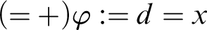
 $$ \begin{align*} (=+) \ \frac{{ \varphi[x/t_2], \Gamma \!\!\Rightarrow \Delta}}{{t_1\approx t_2, \varphi[x/t_1], \Gamma \!\!\Rightarrow \Delta}} & (= -) \ \frac{{b=b, \Gamma \!\!\Rightarrow \Delta}}{{\Gamma \!\!\Rightarrow \Delta}} \end{align*} $$
where
 $\varphi $
is elementary in
$\varphi $
is elementary in
 $(=+)$
and
$(=+)$
and
 $t_1\approx t_2$
means that either
$t_1\approx t_2$
means that either
 $t_1=t_2$
or
$t_1=t_2$
or
 $t_2=t_1$
occurs (so there are two rules in fact). And:
$t_2=t_1$
occurs (so there are two rules in fact). And:
 $$ \begin{align*} (Str) \ \frac{{a=d, \Gamma \!\!\Rightarrow \Delta}}{{\varphi[x/d], \Gamma \!\!\Rightarrow \Delta}} &\quad (Str_=) \ \frac{{a=d_i, \Gamma \!\!\Rightarrow \Delta}}{{d_1=d_2, \Gamma \!\!\Rightarrow \Delta}} \end{align*} $$
where
 $\varphi $
is q-atomic (contains at least one occurrence of d) and
$\varphi $
is q-atomic (contains at least one occurrence of d) and
 $i\in \{1, 2\}$
in
$i\in \{1, 2\}$
in
 $(Str_=)$
; a is not in
$(Str_=)$
; a is not in
 $\Gamma , \Delta , \varphi $
.
$\Gamma , \Delta , \varphi $
.
 $(Str_=)$
is in fact a special case of
$(Str_=)$
is in fact a special case of
 $(Str)$
but it is better to display it as a rule on its own, as in KMM. The name is for ‘strict’ predicate in the sense applied in Reference Feferman[4].
$(Str)$
but it is better to display it as a rule on its own, as in KMM. The name is for ‘strict’ predicate in the sense applied in Reference Feferman[4].
For descriptions we have the following pair of symmetric rules (briefly called DD-rules):


where a (the eigenvariable) is not in
 $\Gamma , \Delta , \varphi $
and
$\Gamma , \Delta , \varphi $
and
 $b, c$
is any parameter.
$b, c$
is any parameter.
Let us pause for the moment to comment on these rules.
 $(=-)$
is just
$(=-)$
is just
 $(ID)$
.
$(ID)$
.
 $(=+)$
corresponds to
$(=+)$
corresponds to
 $(LL)$
but with two significant differences. First, it is restricted to elementary formulae, whereas
$(LL)$
but with two significant differences. First, it is restricted to elementary formulae, whereas
 $(LL)$
admits replacement in arbitrary ones. We explained in the preceding subsection why such restriction is needed. Second, there are two possible positions of substituted argument. It has the result that symmetry for all mixed identities can be proved in the simpler way; the more complicated argument, according to the lines of the proof from the last subsection, is required only for d-identity. This issue is related to the next two rules corresponding to denotation principles. In contrast to the latter, these are not axioms but rules, directly introduce (in the premiss) an eigenvariable a and uniformly do it for only one (selected) term occurring in the conclusion. Moreover, in contrast to denotation principles they are restricted to descriptions only. In particular,
$(LL)$
admits replacement in arbitrary ones. We explained in the preceding subsection why such restriction is needed. Second, there are two possible positions of substituted argument. It has the result that symmetry for all mixed identities can be proved in the simpler way; the more complicated argument, according to the lines of the proof from the last subsection, is required only for d-identity. This issue is related to the next two rules corresponding to denotation principles. In contrast to the latter, these are not axioms but rules, directly introduce (in the premiss) an eigenvariable a and uniformly do it for only one (selected) term occurring in the conclusion. Moreover, in contrast to denotation principles they are restricted to descriptions only. In particular,
 $(Str_=)$
cannot be applied to mixed identity and this is the reason why
$(Str_=)$
cannot be applied to mixed identity and this is the reason why
 $(=+)$
is formulated in the way allowing to cover the symmetric case.
$(=+)$
is formulated in the way allowing to cover the symmetric case.
Both DD-rules are counterparts of
 $(RD)$
. Let us comment on the restriction of DD-rules to mixed identities, moreover, with the strictly imposed order: parameter as the left and DD as the right argument. In fact, the more general form of the rule with arbitrary t instead of c is correct. However, we will see that restriction to mixed identities is sufficient to prove interderivability of our DD-rules with
$(RD)$
. Let us comment on the restriction of DD-rules to mixed identities, moreover, with the strictly imposed order: parameter as the left and DD as the right argument. In fact, the more general form of the rule with arbitrary t instead of c is correct. However, we will see that restriction to mixed identities is sufficient to prove interderivability of our DD-rules with
 $(RD)$
and for some technical reasons it appears more convenient to assume rules of this form. On the other hand, one may doubt whether this solution is not too restrictive. These are connected with the problem of symmetry of identity (mixed and d-identities) and with the question of how to deal with d-identities in the course of proof-search if DD-rules are restricted to mixed identities. And one can ask if it is not better to relax either the proviso concerning the kind of identities or the position of the principal term. The more general form of DD-rules admitting d-identities may seem more natural from the proof-search perspective and one can ask what to do with d-identities if we want to apply DD-rules to one of their argument. This is not a problem. If we have a d-identity in the antecedent we can obtain mixed identity suitable for the application of
$(RD)$
and for some technical reasons it appears more convenient to assume rules of this form. On the other hand, one may doubt whether this solution is not too restrictive. These are connected with the problem of symmetry of identity (mixed and d-identities) and with the question of how to deal with d-identities in the course of proof-search if DD-rules are restricted to mixed identities. And one can ask if it is not better to relax either the proviso concerning the kind of identities or the position of the principal term. The more general form of DD-rules admitting d-identities may seem more natural from the proof-search perspective and one can ask what to do with d-identities if we want to apply DD-rules to one of their argument. This is not a problem. If we have a d-identity in the antecedent we can obtain mixed identity suitable for the application of
 $(\imath \Rightarrow )$
by using
$(\imath \Rightarrow )$
by using
 $(Str_=)$
first. In case we have a d-identity in the succedent, the following strategy always makes possible to change it into mixed identities ready to go for
$(Str_=)$
first. In case we have a d-identity in the succedent, the following strategy always makes possible to change it into mixed identities ready to go for
 $(\Rightarrow \imath )$
:
$(\Rightarrow \imath )$
:

Hence restriction to mixed identities as principal formulae of DD-rules is not essential. On the other hand, if we admit d-identities we must keep the restriction concerning the order. It is not important if DD is the right or the left argument but it must be fixed; otherwise the proof of cut elimination fails if cut formula is a d-identity introduced in both premisses by means of DD-rules but operating not on the same term (and assuming that they are not identical). This shows that taking DD-rules with mixed identities may be more convenient.
In particular, it will be essential for the improved system where allowing two variants of DD-rules with either
 $c=d$
or
$c=d$
or
 $d=c$
will be necessary. For the time being one variant is sufficient since symmetry holds for mixed and d-identities. Since, due to symmetric variant of
$d=c$
will be necessary. For the time being one variant is sufficient since symmetry holds for mixed and d-identities. Since, due to symmetric variant of
 $(=+)$
, the standard proof works for both mixed identities, we must only show that it works for d-identities. The proof goes like this:
$(=+)$
, the standard proof works for both mixed identities, we must only show that it works for d-identities. The proof goes like this:

where in the first (from the root) application of
 $(=+) \varphi := d=x$
, and in the second
$(=+) \varphi := d=x$
, and in the second
 $\varphi := x=d$
.
$\varphi := x=d$
.
3.3. Adequacy of LKID1
In order to show the equivalence of LKID1 and LKID0 we must remember that
 $(=+)$
is weaker than
$(=+)$
is weaker than
 $(LL)$
. Hence first we must prove:
$(LL)$
. Hence first we must prove:
Lemma 3.6 (Leibniz Law)
LKID1
 $\vdash t_1=t_2, \varphi [x/t_1] \Rightarrow \varphi [x/t_2]$
, for any formula
$\vdash t_1=t_2, \varphi [x/t_1] \Rightarrow \varphi [x/t_2]$
, for any formula
 $\varphi $
.
$\varphi $
.
Proof. The proof is by induction on the construction of
 $\varphi $
. In the basis
$\varphi $
. In the basis
 $\varphi $
is elementary; hence it holds by
$\varphi $
is elementary; hence it holds by
 $(=+)$
. The proof of the induction step is standard.□
$(=+)$
. The proof of the induction step is standard.□
Thus we have shown that
 $(=+)$
is as strong as
$(=+)$
is as strong as
 $(LL)$
and we are in a position to prove:
$(LL)$
and we are in a position to prove:
Theorem 3.7. If LKID0
 $\vdash \Gamma \Rightarrow \Delta $
, then LKID1
$\vdash \Gamma \Rightarrow \Delta $
, then LKID1
 $\vdash \Gamma \Rightarrow \Delta $
.
$\vdash \Gamma \Rightarrow \Delta $
.
Proof. Since every application of
 $(LL)$
in LKID0 is simulated in LKID1 by cut made on Lemma 3.6 as the left premiss with the premiss of this application of
$(LL)$
in LKID0 is simulated in LKID1 by cut made on Lemma 3.6 as the left premiss with the premiss of this application of
 $(LL)$
as the right premiss, it is enough to show that the three axiomatic sequents of LKID0 are provable in LKID1, then the theorem follows by induction on the height of LKID0
$(LL)$
as the right premiss, it is enough to show that the three axiomatic sequents of LKID0 are provable in LKID1, then the theorem follows by induction on the height of LKID0
 $\vdash \Gamma \Rightarrow \Delta $
.
$\vdash \Gamma \Rightarrow \Delta $
.
The proofs of sequents corresponding to both denotation principles are trivial. Let us take as an example
 $Rbd \Rightarrow \exists xx=b \wedge \exists xx=d$
:
$Rbd \Rightarrow \exists xx=b \wedge \exists xx=d$
:

both branches show different ways of proving the cases of
 $t_i$
being a parameter and a description. For
$t_i$
being a parameter and a description. For
 $(DP$
-
$(DP$
-
 $2)$
the proof also depends on the kind of identity and the status of
$2)$
the proof also depends on the kind of identity and the status of
 $t_i$
. In case
$t_i$
. In case
 $t_1$
is a parameter we have:
$t_1$
is a parameter we have:

In case
 $t_1$
is d, the proof depends on the type of
$t_1$
is d, the proof depends on the type of
 $t_2$
and we have either:
$t_2$
and we have either:

or:

where symmetric variant of
 $(=+)$
is applied with b as
$(=+)$
is applied with b as
 $t_2$
and
$t_2$
and
 $\varphi := b=x$
. Note that in this case we cannot just use
$\varphi := b=x$
. Note that in this case we cannot just use
 $(Str_=)$
like in the preceding proof since this rule applies only to d-identities.
$(Str_=)$
like in the preceding proof since this rule applies only to d-identities.
The proof of
 $(RD)$
is slightly more complicated. Let
$(RD)$
is slightly more complicated. Let
 ${\cal D}_1$
be:
${\cal D}_1$
be:

where all leaves are provable by weakening. Let
 ${\cal D}_2$
be:
${\cal D}_2$
be:

then by
 $(\Rightarrow \leftrightarrow )$
on their roots followed by
$(\Rightarrow \leftrightarrow )$
on their roots followed by
 $(\Rightarrow \forall )$
we obtain
$(\Rightarrow \forall )$
we obtain
 $\Rightarrow \forall x(x=\imath y\varphi \leftrightarrow \forall y(\varphi \leftrightarrow y=x)) $
.□
$\Rightarrow \forall x(x=\imath y\varphi \leftrightarrow \forall y(\varphi \leftrightarrow y=x)) $
.□
Theorem 3.8. If LKID1
 $\vdash \Gamma \Rightarrow \Delta $
, then LKID0
$\vdash \Gamma \Rightarrow \Delta $
, then LKID0
 $\vdash \Gamma \Rightarrow \Delta $
.
$\vdash \Gamma \Rightarrow \Delta $
.
Proof. It goes again by induction on the height of
 $\vdash \Gamma \Rightarrow \Delta $
but now it requires derivability of specific rules of LKID1 in LKID0.
$\vdash \Gamma \Rightarrow \Delta $
but now it requires derivability of specific rules of LKID1 in LKID0.
One variant of
 $(=+)$
is just a special case of
$(=+)$
is just a special case of
 $(LL)$
whereas the other is derivable by symmetry of identity. Showing derivability of
$(LL)$
whereas the other is derivable by symmetry of identity. Showing derivability of
 $(Str)$
and
$(Str)$
and
 $(Str_=)$
in the presence of denotation principles as additional axioms is also easy. For
$(Str_=)$
in the presence of denotation principles as additional axioms is also easy. For
 $(Str)$
it looks like that:
$(Str)$
it looks like that:

where
 $\varphi [x/d]$
is of the form
$\varphi [x/d]$
is of the form
 $R^nt_1\ldots t_n$
with
$R^nt_1\ldots t_n$
with
 $d:= t_i$
and
$d:= t_i$
and
 $ \vdots $
comprises a standard proof leading from a conjunction to one of its members obtained by means of
$ \vdots $
comprises a standard proof leading from a conjunction to one of its members obtained by means of
 $(Cut), (W \Rightarrow )$
and
$(Cut), (W \Rightarrow )$
and
 $(\wedge \Rightarrow )$
.
$(\wedge \Rightarrow )$
.
Derivability of both rules for DD in LKID0 is straightforward. Notice that:
(a)
 $\Rightarrow c=\imath x\varphi \leftrightarrow \forall y(\varphi \leftrightarrow y=c) $
is provable by
 $(\forall \Rightarrow )$
on axiom and cut with
$(\forall \Rightarrow )$
on axiom and cut with
 $(RD)$
. Since for any
$(RD)$
. Since for any
 $\varphi , \psi $
, the sequents
$\varphi , \psi $
, the sequents
 $\varphi \leftrightarrow \psi , \varphi \Rightarrow \psi $
and
$\varphi \leftrightarrow \psi , \varphi \Rightarrow \psi $
and
 $\varphi \leftrightarrow \psi , \psi \Rightarrow \varphi $
are provable, then by cut with (a) we obtain:
$\varphi \leftrightarrow \psi , \psi \Rightarrow \varphi $
are provable, then by cut with (a) we obtain:
(b)
 $c=\imath x\varphi \Rightarrow \forall y(\varphi \leftrightarrow y=c)$
and
$c=\imath x\varphi \Rightarrow \forall y(\varphi \leftrightarrow y=c)$
and
(c)
 $\forall y(\varphi \leftrightarrow y=c)\Rightarrow c=\imath x\varphi $
.
$\forall y(\varphi \leftrightarrow y=c)\Rightarrow c=\imath x\varphi $
.
From the premisses of
 $(\imath \Rightarrow )$
we deduce:
$(\imath \Rightarrow )$
we deduce:

which, by cut with (b) yields the conclusion of
 $(\imath \Rightarrow )$
. In a similar way we deduce
$(\imath \Rightarrow )$
. In a similar way we deduce
 $\Gamma \Rightarrow \Delta , \forall y(\varphi \leftrightarrow y=c)$
from premisses of
$\Gamma \Rightarrow \Delta , \forall y(\varphi \leftrightarrow y=c)$
from premisses of
 $(\Rightarrow \imath )$
, and by cut with (c) we obtain the conclusion of this rule.□
$(\Rightarrow \imath )$
, and by cut with (c) we obtain the conclusion of this rule.□
On the basis of Theorems 3.5, 3.7 and 3.8 we obtain:
Theorem 3.9. LKID1 is an adequate formalization of KMM.
3.4. Cut elimination problem
LKID1 is more standard SC than LKID0. In particular, it has no additional axioms but instead a pair of symmetric rules (of introduction of the constant to the antecedent and to the succedent) for DD which are reductive. The substitution lemma (i.e., part 1 of Theorem 2.2) also holds for this system in the same form as it was stated for LK. Note that the more general result where arbitrary terms are substituted for parameters cannot be proved here, since it would justify unrestricted
 $(ID)$
for arbitrary
$(ID)$
for arbitrary
 $t=t$
. However, in all quantifier rules instantiation is also restricted to parameters; hence this restricted form of the lemma is sufficient for all transformations required in the proof of cut elimination.
$t=t$
. However, in all quantifier rules instantiation is also restricted to parameters; hence this restricted form of the lemma is sufficient for all transformations required in the proof of cut elimination.
We could expect that due to the restriction on
 $(=+)$
we can avoid also the problems with r-reduction described in Section 3.1. Indeed there is no problem for the old rules already present in LKID0. However, LKID1 still cannot be proved to be cut-free in the presence of our symmetric DD rules. The problem is that the principal formulae of these rules are identities and the clash is possible with cut formula being mixed identity but active in the application of
$(=+)$
we can avoid also the problems with r-reduction described in Section 3.1. Indeed there is no problem for the old rules already present in LKID0. However, LKID1 still cannot be proved to be cut-free in the presence of our symmetric DD rules. The problem is that the principal formulae of these rules are identities and the clash is possible with cut formula being mixed identity but active in the application of
 $(=+)$
. Consider the following cut application:
$(=+)$
. Consider the following cut application:

In this case neither h-reduction nor r-reduction is possible. Generally, the problem is that even if we have a pair of logical rules which are reductive with each other (and this is the case of DD-rules) it is not sufficient for cut elimination if there are other logical rules which introduce principal formulae of the same shape. The problem is not merely that we are unable to provide a constructive proof of the cut elimination theorem. Consider the following proof:

Without cut we cannot prove this sequent in LKID1. There are at least two ways to repair the situation. As we mentioned in Section 3.1,
 $(LL)$
may be represented by other rules. One way out is to change
$(LL)$
may be represented by other rules. One way out is to change
 $(=+)$
for:
$(=+)$
for:

The new rule is interderivable with
 $(=+)$
in the following way:
$(=+)$
in the following way:

and

Hence the variant of LKID1 with
 $(=)$
replacing
$(=)$
replacing
 $(=+)$
is equivalent to the original one. The sequent
$(=+)$
is equivalent to the original one. The sequent
 $Aa, \forall x(Ax\rightarrow x=a) \Rightarrow A\imath xAx$
may be easily proven using
$Aa, \forall x(Ax\rightarrow x=a) \Rightarrow A\imath xAx$
may be easily proven using
 $(=)$
instead of
$(=)$
instead of
 $(Cut)$
. Moreover, we avoid the aforementioned problem with the clash of mixed identities and we can prove cut elimination. Such a solution was applied successfully for sequent calculi for several free logics with definite descriptions in Reference Indrzejczak[9]. There are some costs however, since the subformula property fails for the variant of LKID1 with
$(Cut)$
. Moreover, we avoid the aforementioned problem with the clash of mixed identities and we can prove cut elimination. Such a solution was applied successfully for sequent calculi for several free logics with definite descriptions in Reference Indrzejczak[9]. There are some costs however, since the subformula property fails for the variant of LKID1 with
 $(=)$
. From the point of view of proof-search it is not problematic; it is rather obvious that
$(=)$
. From the point of view of proof-search it is not problematic; it is rather obvious that
 $(=)$
must be applied only for identities already present below and no fresh elementary formulae need be used. But we can do even better and this is the second way out of the problem. The main contribution of this paper is to show that by means of more fine grained syntactical analysis it is possible to obtain a system which satisfies both constructive cut elimination and the subformula property.
$(=)$
must be applied only for identities already present below and no fresh elementary formulae need be used. But we can do even better and this is the second way out of the problem. The main contribution of this paper is to show that by means of more fine grained syntactical analysis it is possible to obtain a system which satisfies both constructive cut elimination and the subformula property.
4. The main result
4.1. LKID2—an improved approach
A careful analysis of identity is a distinctive feature of the present system. Instead of
 $(=+)$
or
$(=+)$
or
 $(=)$
, a collection of term-sensitive rules is introduced which are pairwise reductive and enable not only cut elimination but the preservation of the subformula property. In addition to LK we have the following rules:
$(=)$
, a collection of term-sensitive rules is introduced which are pairwise reductive and enable not only cut elimination but the preservation of the subformula property. In addition to LK we have the following rules:
A. Instead of
 $(Str)$
there are:
$(Str)$
there are:
 $$ \begin{align*} &(Str \Rightarrow) \ \frac{{a_1=d_1, \ldots, a_n=d_n, \varphi[x_1/a_1 \ldots x_n/a_n], \Gamma \!\!\Rightarrow \Delta}}{{\varphi[x_1/d_1 \ldots x_n/d_n], \Gamma \!\!\Rightarrow \Delta}}\\ &(\Rightarrow Str) \ \frac{{\Gamma_1 \!\!\Rightarrow \Delta_1, b_1=d_1 \hspace{.5cm} \ldots \hspace{.5cm} \Gamma_n \!\!\Rightarrow \Delta_n, b_n=d_n \hspace{.5cm}\Gamma_{n+1} \!\!\Rightarrow \Delta_{n+1}, \varphi[x_1/b_1 \ldots x_n/b_n] }}{{\Gamma \!\!\Rightarrow \Delta, \varphi[x_1/d_1 \ldots x_n/d_n]}} \end{align*} $$
where
 $\varphi [x_1/d_1 \ldots x_n/d_n]$
is a proper quasi-atomic formula with exactly
$\varphi [x_1/d_1 \ldots x_n/d_n]$
is a proper quasi-atomic formula with exactly
 $n \geq 1$
different definite descriptions (with possibly many occurrences) as arguments, and
$n \geq 1$
different definite descriptions (with possibly many occurrences) as arguments, and
 $\varphi [x_1/b_1 \ldots x_n/b_n] $
is a proper atomic one (i.e., with no DD). Every
$\varphi [x_1/b_1 \ldots x_n/b_n] $
is a proper atomic one (i.e., with no DD). Every
 $a_i$
in
$a_i$
in
 $(Str\Rightarrow )$
is an eigenvariable so they must be different from each other as well. It is important to make the substitution and the corresponding generation of mixed identities in one step on all (occurrences) of DD since this guarantees that reduction step in cut elimination proof is possible. Otherwise we could have for example
$(Str\Rightarrow )$
is an eigenvariable so they must be different from each other as well. It is important to make the substitution and the corresponding generation of mixed identities in one step on all (occurrences) of DD since this guarantees that reduction step in cut elimination proof is possible. Otherwise we could have for example
 $Rd_1d_2$
as the cut formula where the rule was applied to two different arguments in both premisses of cut and this destroys the possibility of cut-rank reduction.
$Rd_1d_2$
as the cut formula where the rule was applied to two different arguments in both premisses of cut and this destroys the possibility of cut-rank reduction.
B. As the counterpart of
 $(Str_=)$
we have a pair of symmetric rules for d-identities:
$(Str_=)$
we have a pair of symmetric rules for d-identities:
 $$ \begin{align*} &( =\Rightarrow) \ \frac{{a_1= d_1, a_2= d_2, a_1=a_2, \Gamma \!\!\Rightarrow \Delta}}{{d_1= d_2, \Gamma \!\!\Rightarrow \Delta}}\\ &(\Rightarrow =) \ \frac{{\Gamma_1 \!\!\Rightarrow \Delta_1, b=d_1 \hspace{.5cm} \Gamma_2 \!\!\Rightarrow \Delta_2, c= d_2 \hspace{.5cm} \Gamma_3 \!\!\Rightarrow \Delta_3, b=c }}{{\Gamma \!\!\Rightarrow \Delta, d_1= d_2}} \end{align*} $$
where
 $a_1, a_2$
in
$a_1, a_2$
in
 $(=\Rightarrow )$
are different eigenvariables.
$(=\Rightarrow )$
are different eigenvariables.
C. For mixed identities we have the rules for DD which are essentially the same as in LKID1 but they are doubled in the sense that conclusion of each rule may be either
 $c=d$
or
$c=d$
or
 $d=c$
. So we have in fact four rules:
$d=c$
. So we have in fact four rules:
 $$ \begin{align*} &(\imath\Rightarrow) \ \frac{{\Gamma_1 \!\!\Rightarrow \Delta_1, \varphi[x/b], b=c \ [c=b]\hspace{.5cm} b = c \ [c=b], \varphi[x/b], \Gamma_2 \!\!\Rightarrow \Delta_2}}{{c=\imath x \varphi \ [\imath x\varphi =c], \Gamma \!\!\Rightarrow \Delta }}\\ &(\Rightarrow\imath) \ \frac{{a=c \ [c=a], \Gamma_1 \!\!\Rightarrow \Delta_1, \varphi[x/a] \hspace{.5cm}\varphi[x/a], \Gamma_2 \!\!\Rightarrow \Delta_2, a=c \ [c=a]}}{{\Gamma \!\!\Rightarrow \Delta, c=\imath x \varphi \ [\imath x\varphi =c]}} \end{align*} $$
where the alternative conclusion and premiss is put in square brackets. Again a is the eigenvariable of
 $(\Rightarrow \imath )$
.
$(\Rightarrow \imath )$
.
D. For atomic identities we have:
 $$ \begin{align*} (R) \ \frac{{b=b, \Gamma \!\!\Rightarrow \Delta}}{{\Gamma \!\!\Rightarrow \Delta}} \hspace{.1cm} (E) \ \frac{{b=c, \Gamma \!\!\Rightarrow \Delta }}{{a=b, a=c, \Gamma \!\!\Rightarrow \Delta}} \hspace{.1cm} (L) \ \frac{{\varphi[x/b], \Gamma \!\!\Rightarrow \Delta }}{{a=b, \varphi[x/a], \Gamma \!\!\Rightarrow \Delta}} \end{align*} $$
where
 $\varphi $
is a proper atomic formula.
$\varphi $
is a proper atomic formula.
One can easily observe that, in contrast to LKID1, there is a strict division of labor between rules introducing identities with different kind of arguments as principal formulae.
 $(R), (E), (L)$
(for reflexivity, Euclid and Leibniz) deal only with atomic identities,
$(R), (E), (L)$
(for reflexivity, Euclid and Leibniz) deal only with atomic identities,
 $(=\Rightarrow )$
and
$(=\Rightarrow )$
and
 $(\Rightarrow =)$
with d-identities and
$(\Rightarrow =)$
with d-identities and
 $\imath $
-rules with mixed identities. Both
$\imath $
-rules with mixed identities. Both
 $Str$
-rules complete the picture. All rules, except those in the last group, are symmetric and, as we shall see, reductive. The important thing is that all rules (except cut) satisfy the subformula property. In particular, no rule admits in the premisses any DD which is not present in the conclusion of the rule.
$Str$
-rules complete the picture. All rules, except those in the last group, are symmetric and, as we shall see, reductive. The important thing is that all rules (except cut) satisfy the subformula property. In particular, no rule admits in the premisses any DD which is not present in the conclusion of the rule.
If we take a restricted language with parameters as the only terms the three rules from the last group are sufficient to obtain the system LKI for pure FOL with identity; by
 $(E)$
we prove symmetry and transitivity of = and
$(E)$
we prove symmetry and transitivity of = and
 $(L)$
is sufficient to prove suitable congruence principles for predicates of arbitrary arity. The remaining six (or rather eight) rules are necessary not only to characterize DD but also to restore the usual behavior of = in the presence of DD.
$(L)$
is sufficient to prove suitable congruence principles for predicates of arbitrary arity. The remaining six (or rather eight) rules are necessary not only to characterize DD but also to restore the usual behavior of = in the presence of DD.
As an example of proof we show again the equivalence of
 $\exists x x=t$
and
$\exists x x=t$
and
 $t=t$
.
$t=t$
.
For
 $\exists xx=b\leftrightarrow b=b$
it is almost the same as in LKID0; only
$\exists xx=b\leftrightarrow b=b$
it is almost the same as in LKID0; only
 $(\Rightarrow \exists )$
must be additionally applied in the rightmost leaf. For
$(\Rightarrow \exists )$
must be additionally applied in the rightmost leaf. For
 $\exists xx=d\leftrightarrow d=d$
we have:
$\exists xx=d\leftrightarrow d=d$
we have:

where
 ${\cal D}$
is:
${\cal D}$
is:

4.2. Soundness
It is not problematic to show that the new calculus LKID2 is not stronger than the former LKID1. We will show:
Theorem 4.10. If LKID2
 $\vdash \Gamma \Rightarrow \Delta $
, then LKID1
$\vdash \Gamma \Rightarrow \Delta $
, then LKID1
 $\vdash \Gamma \Rightarrow \Delta $
.
$\vdash \Gamma \Rightarrow \Delta $
.
Proof.
 $(E)$
and
$(E)$
and
 $(L)$
are just special cases of
$(L)$
are just special cases of
 $(=+)$
. Two variants of the present versions of
$(=+)$
. Two variants of the present versions of
 $(\imath \Rightarrow ), (\Rightarrow \imath )$
are rules of LKID1. The other two are just symmetric versions of the former rules for DD and we have shown that identity is symmetric in LKID1 for any terms. Hence we must only demonstrate that the remaining new rules are derivable in LKID1. In case of both
$(\imath \Rightarrow ), (\Rightarrow \imath )$
are rules of LKID1. The other two are just symmetric versions of the former rules for DD and we have shown that identity is symmetric in LKID1 for any terms. Hence we must only demonstrate that the remaining new rules are derivable in LKID1. In case of both
 $Str$
-rules we restrict proofs to the case with only one DD present in atomic
$Str$
-rules we restrict proofs to the case with only one DD present in atomic
 $\varphi $
to avoid unnecessarily complicated proof schemata. It is obvious how to prove derivability for arbitrary n distinct descriptions.
$\varphi $
to avoid unnecessarily complicated proof schemata. It is obvious how to prove derivability for arbitrary n distinct descriptions.
For
 $(\Rightarrow Str)$
:
$(\Rightarrow Str)$
:

For
 $(Str\Rightarrow )$
:
$(Str\Rightarrow )$
:

For
 $(=\Rightarrow )$
it goes similarly:
$(=\Rightarrow )$
it goes similarly:

For
 $(\Rightarrow =)$
it is enough to prove:
$(\Rightarrow =)$
it is enough to prove:

and apply cut thrice with the premisses of
 $(\Rightarrow =)$
.□
$(\Rightarrow =)$
.□
4.3. Completeness
The opposite direction, i.e., a proof that the new system is strong enough to prove everything provable in the former system requires demonstration that both
 $(E)$
and
$(E)$
and
 $(L)$
can be strengthened to cover the full power of
$(L)$
can be strengthened to cover the full power of
 $(=+)$
.
$(=+)$
.
Let us first consider the following additional rules:
 $$ \begin{align*} (S) \ \frac{{t_2=t_1, \Gamma \!\!\Rightarrow \Delta}}{{t_1=t_2, \Gamma \!\!\Rightarrow \Delta}} \hspace{.1cm} (E') \ \frac{{t_2=t_3, \Gamma \!\!\Rightarrow \Delta }}{{t_1=t_2, t_1=t_3, \Gamma \!\!\Rightarrow \Delta}} \hspace{.1cm} (L') \ \frac{{\varphi[x/t_2], \Gamma \!\!\Rightarrow \Delta }}{{t_1=t_2, \varphi[x/t_1], \Gamma \!\!\Rightarrow \Delta}} \end{align*} $$
where
 $\varphi $
is a proper elementary formula.
$\varphi $
is a proper elementary formula.
First we prove:
Lemma 4.11.
 $(S)$
is derivable in LKID2.
$(S)$
is derivable in LKID2.
Proof. It is sufficient to prove
 $t_1=t_2\Rightarrow t_2=t_1$
since by cut with the premiss of
$t_1=t_2\Rightarrow t_2=t_1$
since by cut with the premiss of
 $(S)$
it yields its conclusion. Symmetry of atomic identities is guaranteed by
$(S)$
it yields its conclusion. Symmetry of atomic identities is guaranteed by
 $(R), (E)$
. For mixed identities
$(R), (E)$
. For mixed identities
 $b=d$
and
$b=d$
and
 $d=b$
it holds by
$d=b$
it holds by
 $(\imath \Rightarrow ), (\Rightarrow \imath )$
in the following way:
$(\imath \Rightarrow ), (\Rightarrow \imath )$
in the following way:

where proofs of both premisses are:

and:

It remains to prove it for d-identity
 $d_1=d_2\Rightarrow d_2=d_1$
to ensure that identity is symmetric on all possible arguments:
$d_1=d_2\Rightarrow d_2=d_1$
to ensure that identity is symmetric on all possible arguments:

(incidentally the rightmost branches in two preceding proofs cover the case of atomic identities). Hence symmetry holds generally and we will be using
 $(S)$
below to simplify other proofs.□
$(S)$
below to simplify other proofs.□
It is interesting to note why in LKID2 we need four DD-rules instead of two like in LKID1. In the latter system the proof of symmetry for mixed identities was directly obtained by
 $(=+)$
and
$(=+)$
and
 $(=-)$
on
$(=-)$
on
 $c=c$
. But in LKID2 there is a division of labor between several rules dealing with identity. In particular,
$c=c$
. But in LKID2 there is a division of labor between several rules dealing with identity. In particular,
 $(L)$
can be applied only on atomic identities as principal formulae and we cannot mimic the proof from LKID1 if the identity is mixed. Hence the addition of symmetric variants of DD-rules is necessary; otherwise cut is not eliminable from LKID2.
$(L)$
can be applied only on atomic identities as principal formulae and we cannot mimic the proof from LKID1 if the identity is mixed. Hence the addition of symmetric variants of DD-rules is necessary; otherwise cut is not eliminable from LKID2.
Lemma 4.12.
 $(E')$
is derivable in LKID2.
$(E')$
is derivable in LKID2.
Proof. As before it is sufficient to prove
 $t_1=t_2, t_1=t_3\Rightarrow t_2=t_3$
and apply cut to the premiss of
$t_1=t_2, t_1=t_3\Rightarrow t_2=t_3$
and apply cut to the premiss of
 $(E')$
. Since for the case of all terms being parameters it holds by
$(E')$
. Since for the case of all terms being parameters it holds by
 $(E)$
we must prove the following combinations:
$(E)$
we must prove the following combinations:
-
1.
$b=c, b=d \Rightarrow c=d$
; -
2.
$b=d, b=c \Rightarrow d=c$
; -
3.
$d=b, d=c\Rightarrow b=c$
; -
4.
$d_1=d_2, d_1=b\Rightarrow d_2=b$
; -
5.
$d_1=b, d_1=d_2\Rightarrow b=d_2$
; -
6.
$b=d_1, b=d_2\Rightarrow d_1=d_2$
; -
7.
$d_1=d_2, d_1=d_3\Rightarrow d_2=d_3$
.


These cases cover all possible combinations of parameters and descriptions as arguments. ad 1 (
 $d :=\imath x\varphi $
):
$d :=\imath x\varphi $
):

where
 ${\cal D}$
is:
${\cal D}$
is:

ad 2: It holds by 1 and symmetry on
 $c=d$
.
$c=d$
.
ad 3:

ad 4:

where both leaves are provable; the left by 3, the right by 2.
ad 5: by 4 and symmetry on
 $d_2=b$
.
$d_2=b$
.
ad 6:

ad 7:

where
 $S_1, S_2$
are axiomatic sequents
$S_1, S_2$
are axiomatic sequents
 $b= d_2\Rightarrow b= d_2 $
and
$b= d_2\Rightarrow b= d_2 $
and
 $c= d_3\Rightarrow c= d_3 $
, and the next leaf to the right is provable by 3 and
$c= d_3\Rightarrow c= d_3 $
, and the next leaf to the right is provable by 3 and
 $(S)$
on
$(S)$
on
 $d_1=a, d_1=a'$
.□
$d_1=a, d_1=a'$
.□
Lemma 4.13.
 $(L')$
is derivable in LKID2.
$(L')$
is derivable in LKID2.
Proof. Again it is sufficient to prove
 $t_1=t_2, \varphi [x/t_1]\Rightarrow \varphi [x/t_2]$
for arbitrary terms and proper elementary formula
$t_1=t_2, \varphi [x/t_1]\Rightarrow \varphi [x/t_2]$
for arbitrary terms and proper elementary formula
 $\varphi $
.
$\varphi $
.
-
1.
$b=c, \varphi [x/b]\Rightarrow \varphi [x/c]$
. -
2.
$b=d, \varphi [x/b]\Rightarrow \varphi [x/d]$
. -
3.
$d=b, \varphi [x/d]\Rightarrow \varphi [x/b]$
. -
4.
$d_1=d_2, \varphi [x/d_1]\Rightarrow \varphi [x/d_2]$
.


ad 1. In case
 $\varphi $
is a proper atomic formula it follows by
$\varphi $
is a proper atomic formula it follows by
 $(L)$
. Otherwise it has some occurrence of DD and requires additional work:
$(L)$
. Otherwise it has some occurrence of DD and requires additional work:

where
 $S_1 \ldots S_n$
is a number of sequents of the form
$S_1 \ldots S_n$
is a number of sequents of the form
 $a_1= d_1\Rightarrow a_1=d_1 \ \ldots \ a_n= d_n\Rightarrow a_n=d_n $
.
$a_1= d_1\Rightarrow a_1=d_1 \ \ldots \ a_n= d_n\Rightarrow a_n=d_n $
.
ad 2. It holds immediately by
 $(\Rightarrow Str)$
if d is the only DD occurring only in
$(\Rightarrow Str)$
if d is the only DD occurring only in
 $\varphi [x/d]$
. Otherwise we have also some other descriptions in
$\varphi [x/d]$
. Otherwise we have also some other descriptions in
 $\varphi [x/b]$
and we must first apply
$\varphi [x/b]$
and we must first apply
 $(Str\Rightarrow )$
to change them all into parameters. Then the proof goes like in case 1.
$(Str\Rightarrow )$
to change them all into parameters. Then the proof goes like in case 1.
ad 3. Assume for simplifying a proof figure (i.e., to diminish the number of inessential branches) that only one other description is present in
 $\varphi $
:
$\varphi $
:

In case no other DD are present in
 $\varphi $
the application of
$\varphi $
the application of
 $(\Rightarrow Str)$
is not required; in case there is more than one, we simply obtain more axiomatic branches of the form
$(\Rightarrow Str)$
is not required; in case there is more than one, we simply obtain more axiomatic branches of the form
 $a_i=d_i\Rightarrow a_i=d_i$
.
$a_i=d_i\Rightarrow a_i=d_i$
.
ad 4: The proof is similar but with the additional application of
 $(=\Rightarrow )$
as the first (from the root) inference on
$(=\Rightarrow )$
as the first (from the root) inference on
 $d_1=d_2$
.□
$d_1=d_2$
.□
Theorem 4.14. If LKID1
 $\vdash \Gamma \Rightarrow \Delta $
, then LKID2
$\vdash \Gamma \Rightarrow \Delta $
, then LKID2
 $\vdash \Gamma \Rightarrow \Delta $
.
$\vdash \Gamma \Rightarrow \Delta $
.
Proof. Notice that the only difference between
 $(L')$
and
$(L')$
and
 $(=+)$
is that the former does not cover the case where
$(=+)$
is that the former does not cover the case where
 $\varphi $
is an identity. Then to show that the latter is derivable in LKID2 we must consider three cases where
$\varphi $
is an identity. Then to show that the latter is derivable in LKID2 we must consider three cases where
 $\varphi $
is either of the form
$\varphi $
is either of the form
 $x=t$
or
$x=t$
or
 $t=x$
or
$t=x$
or
 $x=x$
for arbitrary t as the second argument. With all possible combinations of parameters and DD as respective terms it gives
$x=x$
for arbitrary t as the second argument. With all possible combinations of parameters and DD as respective terms it gives
 $8+8+4$
subcases in total. Fortunately in most cases proofs are identical. In the first case we obtain a proof by
$8+8+4$
subcases in total. Fortunately in most cases proofs are identical. In the first case we obtain a proof by
 $(E')$
:
$(E')$
:

Similarly in the second case but additionally we must use
 $(S)$
in all subcases:
$(S)$
in all subcases:

In the last case only two terms
 $t_1, t_2$
are present and if both are parameters or if
$t_1, t_2$
are present and if both are parameters or if
 $t_1:= d$
and
$t_1:= d$
and
 $t_2:=b$
, then we obtain a proof by
$t_2:=b$
, then we obtain a proof by
 $(R)$
, and
$(R)$
, and
 $(W\Rightarrow )$
. In the remaining two subcases we obtain the following proofs:
$(W\Rightarrow )$
. In the remaining two subcases we obtain the following proofs:


□
Hence:
Theorem 4.15. LKID2 is an adequate formalization of KMM.
4.4. Cut elimination
From the proof-theoretic standpoint LKID2 is much better-behaved system than LKID1. The substitution lemma holds in the same form as for LKID1; the addition of new rules does not affect the proof of this result. One can easily check that all new rules are pairwise reductive and there is no risk of a clash, as was illustrated for LKID1. In particular, restrictions put on
 $(L)$
(proper atomic formulae) are necessary to avoid a clash with
$(L)$
(proper atomic formulae) are necessary to avoid a clash with
 $(\Rightarrow Str)$
; restrictions on
$(\Rightarrow Str)$
; restrictions on
 $(E)$
(atomic identities) to avoid a clash with
$(E)$
(atomic identities) to avoid a clash with
 $(\Rightarrow =)$
or
$(\Rightarrow =)$
or
 $(\Rightarrow \imath )$
. As a result for all kinds of elementary formulae their role as active formulae in a proof is strictly determined:
$(\Rightarrow \imath )$
. As a result for all kinds of elementary formulae their role as active formulae in a proof is strictly determined:
-
1. if
$\varphi $
is a proper atomic formula, it can be active only in the antecedent, due to
$(L)$
; -
2. if
$\varphi $
is a proper q-atomic, it can be active on both sides but only via
$(Str\Rightarrow )$
and
$(\Rightarrow Str)$
; -
3. if it is a d-identity, it can be active on both sides but only via
$(=\Rightarrow )$
and
$(\Rightarrow =)$
; -
4. if it is a mixed-identity, it can be active on both sides but only via
$(\Rightarrow \imath )$
and
$(\imath \Rightarrow )$
; -
5. if it is an atomic identity, it can be active only in the antecedent, due to
$(E)$
.


Now if an elementary formula is a cut formula, then in cases 1 and 5, its occurrence in the left premiss of cut is always parametric with respect to the rule immediately applied over cut. Hence, h-reduction on the left premiss of cut is always possible. In the remaining three cases, if in at least one premiss it is also parametric, again h-reduction is applicable. But it is also possible that in both premisses of cut, an elementary cut formula was the principal formula of the preceding rules. But, then it was introduced on both sides only by the respective rules which are pairwise reductive; hence r-reduction is possible. We will demonstrate the reductivity of
 $(=\Rightarrow )$
and
$(=\Rightarrow )$
and
 $(\Rightarrow =)$
, and of DD-rules.
$(\Rightarrow =)$
, and of DD-rules.

By the substitution lemma we obtain
 $b_1=d_1, b_2=d_2, b_1=b_2, \Pi \Rightarrow \Sigma $
to unify parameters with those present in the premisses of the application of
$b_1=d_1, b_2=d_2, b_1=b_2, \Pi \Rightarrow \Sigma $
to unify parameters with those present in the premisses of the application of
 $(\Rightarrow =)$
and proceed as follows:
$(\Rightarrow =)$
and proceed as follows:

Note that all cuts are made on cut formulae which have strictly lower rank.
In the case of cut following the application of DD rules:

By the substitution lemma we obtain:
 $$ \begin{align*} \varphi[x/b], \Gamma_1 \Rightarrow \Delta_1, b=c \ \ \ \mbox{and} \ \ \ \ b=c, \Gamma_2 \Rightarrow \Delta_2, \varphi[x/b] \end{align*} $$
from the premisses of
 $\Gamma \Rightarrow \Delta , c=\imath x\varphi $
to unify parameters with those present in the premisses of the application of
$\Gamma \Rightarrow \Delta , c=\imath x\varphi $
to unify parameters with those present in the premisses of the application of
 $(\imath \Rightarrow )$
and proceed as follows:
$(\imath \Rightarrow )$
and proceed as follows:

where the leftmost sequent is obtained in an analogous way by cut on the remaining premisses. All cuts have smaller rank. The last remark applies to all cases of r-reduction. In particular, recall that in the case of identities their rank is always the sum of complexities of arguments, whereas in the case of proper elementary formulae we add 1 to this sum. Note that this is required for the special case of quasi-atomic cut formula introduced by
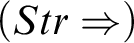 $(Str\Rightarrow )$
and
$(Str\Rightarrow )$
and
 $(\Rightarrow Str)$
, and having just one occurrence of only one d. Then mixed identity
$(\Rightarrow Str)$
, and having just one occurrence of only one d. Then mixed identity
 $a=d$
in premisses is of rank n (the complexity of d), whereas the principal formula of this rule application is of rank
$a=d$
in premisses is of rank n (the complexity of d), whereas the principal formula of this rule application is of rank
 $n+1$
.
$n+1$
.
As we noted in Section 2.4 satisfaction of these conditions is sufficient for proving reduction Lemmata 2.3 and 2.4, and the cut elimination theorem on their basis. Moreover, all rules of LKID2 satisfy the subformula property in the sense of being closed for subformulae and identities where the only new terms are fresh parameters. Hence LKID2 is analytic in the sense that it satisfies both cut elimination and the subformula property in slightly modified form, similar to that which holds for G3 system (see Reference Negri and von Plato[17]).
5. Conclusion
All sequent calculi presented in this paper are weakly equivalent to KMM. But it can be shown also that this logic, after the addition of the definition of definedness predicate of the form
 $\downarrow \!\! t := t=t$
is equivalent to definedness logic (or the logic of partial terms) of Beeson Reference Beeson[2] and Feferman Reference Feferman[4] which was extensively studied and applied in the context of constructive mathematics and computer science. This is a kind of negative free logic with variables fixed as denoting and usually developed on the basis of intuitionistic logic in the context of constructive mathematics. However, Feferman rightly noticed that it works without changes in the classical setting (in fact he provided only classical semantics in Reference Feferman[4]). Indrzejczak Reference Indrzejczak[9] provided a cut-free SC formalization (under the name NQFL for negative quasi-free logic) for both variants of this logic: classical and intuitionistic. NQFL in the classical version is, with some inessential differences, the present system LKID1 (but with
$\downarrow \!\! t := t=t$
is equivalent to definedness logic (or the logic of partial terms) of Beeson Reference Beeson[2] and Feferman Reference Feferman[4] which was extensively studied and applied in the context of constructive mathematics and computer science. This is a kind of negative free logic with variables fixed as denoting and usually developed on the basis of intuitionistic logic in the context of constructive mathematics. However, Feferman rightly noticed that it works without changes in the classical setting (in fact he provided only classical semantics in Reference Feferman[4]). Indrzejczak Reference Indrzejczak[9] provided a cut-free SC formalization (under the name NQFL for negative quasi-free logic) for both variants of this logic: classical and intuitionistic. NQFL in the classical version is, with some inessential differences, the present system LKID1 (but with
 $(=)$
replacing
$(=)$
replacing
 $(=+)$
); hence LKID2 provides an alternative, fully analytic, characterization of classical definedness logic. Moreover, if we change our core system for LJ and in the similar way restrict the additional rules to sequents with at most one formula in the succedent, we obtain the intuitionistic version of LKID2. In particular, both rules
$(=+)$
); hence LKID2 provides an alternative, fully analytic, characterization of classical definedness logic. Moreover, if we change our core system for LJ and in the similar way restrict the additional rules to sequents with at most one formula in the succedent, we obtain the intuitionistic version of LKID2. In particular, both rules
 $(\imath \Rightarrow )$
must be split into:
$(\imath \Rightarrow )$
must be split into:
 $$ \begin{align*} &(\imath\Rightarrow) \ \frac{{\Gamma_1 \!\!\Rightarrow \varphi[x/b]\hspace{.5cm} b = c \ [c=b], \Gamma_2 \!\!\Rightarrow \Delta}}{{c=\imath x \varphi \ [\imath x\varphi =c], \Gamma \!\!\Rightarrow \Delta }}\\ &(\imath\Rightarrow) \ \frac{{\Gamma_1 \!\!\Rightarrow b=c \ [c=b]\hspace{.5cm} \varphi[x/b], \Gamma_2 \!\!\Rightarrow \Delta}}{{c=\imath x \varphi \ [\imath x\varphi =c], \Gamma \!\!\Rightarrow \Delta }} \end{align*} $$
A careful inspection of the proofs shows that all are intuitionistically valid after making suitable corrections. Hence we obtain the intuitionistic theory of RDD in the form of decent SC.
It is an interesting problem for future research to examine the scope of the kind of analysis provided here. In particular, if it may be extended to other kinds of free logics for which cut-free, but not fully analytic, systems were provided in Reference Indrzejczak[9]. This technical problem is somewhat related to more philosophical issue which deserves further study so it will be only signaled here. Dealing via specific sets of rules in LKID2 with different syntactic kinds of identities seems to make them, in a sense, different constants. One may askFootnote 1 what consequences it has for the treatment of identity in the proof-theoretic semantics. Does it really mean that we are dealing with different constants? Elsewhere Reference Indrzejczak[11] I proposed a rather different route to characterization of identity as a logical constant in the setting of a slightly generalized SC with terms being full-fledged elements of sequents (see for example Reference Restall[19] for another SC of this sort). It seems interesting to compare these approaches and proceed with further investigations on this issue.
Acknowledgments
I’m greatly indebted to the referees of this paper for many substantial remarks which helped to improve and extend significantly the final version. The results reported in this paper are supported by the National Science Centre, Poland (grant number: DEC-2017/25/B/HS1/01268).

 Open access