


INTRODUCTION
The main backbone of radiocarbon (14C) calibration has been and will continue to be tree rings dated by dendrochronology, for the time periods where this is possible. Thanks to the work of a large community of scientists in extending our dendrochronological record and generating new 14C measurements, calibration has come a long way since the original curves constructed decades ago (Ralph et al. Reference Ralph, Michael and Han1973; Suess Reference Suess1980; Pearson and Stuiver Reference Pearson and Stuiver1986; Stuiver and Pearson Reference Stuiver and Pearson1986). In the early days, the 14C data were mainly obtained from conventional laboratories specializing in high-precision dating (defined as 2‰ at the time). These were Belfast, Heidelberg, Groningen, Pretoria, Tucson, and Seattle; these laboratories also organized mutual intercomparisons at that time (Kromer et al. Reference Kromer, Ambers, Baillie, Damon, Hesshaimer, Hofmann, Jöris, Levin, Manning and McCormac1996). Today, with IntCal20, the dendro-based calibration curve extends back to 13,910 calBPFootnote 1 (11,960 calBC), with further extensions to 55,000 calBP from other records. Furthermore, large sections of the timescale have been redated using AMS.
Providing a calibration curve beyond our knowledge of dendrochonologically dated tree rings has proved a significant challenge. For the glacial part of the 14C dating range, the first tentative “calibration curves” were based on very few observations, hence were highly coarse and lacking in detail. For example, Vogel and Kronfeld (Reference Vogel and Kronfeld1997) based their curve on only 20 paired 14C and U/Th speleothem observations covering the past 50,000 years. However, during the past few decades, considerable progress has been made. Since the advent of AMS, calibration has been extended gradually to 55,000 years, i.e. the complete dating range, enabled by small samples provided by chronological records other than tree rings. The first dataset spanning the complete 14C dating range was based on varves, i.e. laminated sediments from Lake Suigetsu (Kitagawa and van der Plicht Reference Kitagawa and van der Plicht1998) and further datasets from other archives followed soon thereafter (Beck et al. Reference Beck, Richards, Edwards, Silverman, Smart, Donahue, Hererra-Osterheld, Burr, Calsoyas and Jull2001Footnote 2; Hughen et al. Reference Hughen, Lehman, Southon, Overpeck, Marchal, Herring and Turnbull2004; Fairbanks et al. Reference Fairbanks, Mortlock, Tzu-Chien, Cao, Kaplan, Guilderson, Fairbanks, Bloom, Grootes and Nadeau2005). However, these different records were clearly inconsistent over the oldest part of the 14C dating range, 26–50 ka calBP (van der Plicht Reference van der Plicht2004) and very considerable uncertainties remained (Mellars Reference Mellars2006). For this reason, IntCal04 (Reimer et al. Reference Reimer, Baillie, Bard, Bayliss, Beck, Bertrand, Blackwell, Buck, Burr and Cutler2004) terminated at 26 ka, and no internationally agreed, unified recommendation was made for calibration beyond that age (NotCal04; van der Plicht et al. Reference van der Plicht, Beck, Bard, Baillie, Blackwett, Buck, Friedrich, Guilderson, Hughen and Kromer2004). Instead, radiocarbon users who did wish to calibrate beyond this range were required to select between a wide number of different calibration curves (Weninger and Jöris Reference Weninger, Jöris, Higham, Bronk Ramsey and Owen2004; Fairbanks et al. Reference Fairbanks, Mortlock, Tzu-Chien, Cao, Kaplan, Guilderson, Fairbanks, Bloom, Grootes and Nadeau2005; van Andel Reference van Andel2005; Bronk Ramsey et al. Reference Bronk Ramsey, Buck, Manning, Reimer and van der Plicht2006) based on the various individual datasets, and archives, available. This situation made direct comparability of published “calibrated” ages between studies difficult since potentially different calibration curves had been used to calibrate the underlying radiocarbon ages.
Once the reasons for some of the disparities in the datasets became better understood, the IntCal09 calibration curve (Reimer et al. Reference Reimer, Baillie, Bard, Bayliss, Beck, Blackwell, Bronk Ramsey, Buck, Burr and Edwards2009) was constructed and released to the community. This curve was derived from atmospheric and marine datasets (in particular from the Cariaco basin; Hughen et al. Reference Hughen, Southon, Lehman, Bertrand and Turnbull2006) and corrected for estimated reservoir effects. The IntCal09 curve represented our best estimate of Northern Hemispheric atmospheric 14C at that time. Nevertheless, disparities still remained between this estimate and the only true atmospheric data available of Lake Suigetsu (Kitagawa and van der Plicht Reference Kitagawa and van der Plicht2000), suggesting issues remained to be resolved. Between 2009 and 2013, new records became available, in particular from speleothems (Hulu Cave; Southon et al. Reference Southon, Noronha, Cheng, Lawrence Edwards and Wang2012) and laminated sediments (Lake Suigetsu; Bronk Ramsey et al. Reference Bronk Ramsey, Staff, Bryant, Brock, Kitagawa, van der Plicht, Schlolaut, Marshall, Brauer and Lamb2012). The IntCal13 calibration curve incorporated the information from all of this new data while retaining the information on which IntCal09 was based (Reimer et al. Reference Reimer, Bard, Bayliss, Beck, Blackwell, Bronk Ramsey, Buck, Cheng, Edwards and Friedrich2013).
The new IntCal20 (Reimer et al. Reference Reimer, Austin, Bard, Bayliss, Blackwell, Bronk Ramsey, Butzin, Edwards, Friedrich and Grootes2020 in this issue) is the latest update and revision to the Northern Hemisphere calibration curve. It uses a new statistical methodology (Heaton et al. Reference Heaton, Blaauw, Blackwell, Bronk Ramsey, Reimer and Scott2020a in this issue) throughout which offers more flexibility in modeling and hence an improved ability to combine the varied, and unique, constituent records. In the older time period, it is based upon new insights on various chronologies, most significantly for the Pleistocene (Cheng et al. Reference Cheng, Lawrence Edwards, Southon, Matsumoto, Feinberg, Sinha, Zhou, Li, Li and Xu2018); and improved modeling of marine reservoir effects. We therefore hope IntCal20 moves us further towards resolving the challenges in synthesizing the various archives over this period. Further, the dendrochronological part of the IntCal20 calibration curve is also significantly improved. For example, the dataset for Kauri wood is extended during the Late Glacial (Hogg et al. Reference Hogg, Southon, Turney, Palmer, Bronk Ramsey, Fenwick, Boswijk, Buntgen, Froedrich and Helle2016, Reference Hogg, Heaton, Hua, Bayliss, Blackwell, Boswijk, Ramsey, Palmer, Petchey and Reimer2020 in this issue). It is noteworthy to mention that, in total, IntCal13, the previous calibration curve, was based on 7019 raw measurements; for IntCal20, this number is 12,904.
The work has been revolutionized by measurements using the newly developed MICADAS AMS machines, which are extremely efficient and deliver high-precision dates (Synal et al. Reference Synal, Stocker and Suter2007). Advances in measurement efficiency and enhanced precision will continue to improve the calibration curve further in the coming years (e.g. Balter Reference Balter2006). Annual resolution, dendro-dated, tree ring 14C determinations are being produced at high speed, instigated by the hunt for so-called Miyake events, which are narrow spikes (subannual) of increased 14C production (Miyake et al. Reference Miyake, Nagaya, Masuda and Nakamura2012, Reference Miyake, Masuda and Nakamura2013). In IntCal20, for the first time, these spike events have been specifically incorporated into the curve construction methodology better enabling their retention in the final calibration product (see below for more details). Further, the explosion of annual tree ring data has been incorporated into the curve via the new construction method which also recognizes that other 14C measurements arise from multiple years, commonly decadal, blocks of tree rings.
The present and upcoming single year series therefore enable fine-tuning of the calibration curve for the Holocene and Late Glacial time periods. These high temporal resolution data, improved accuracy in the statistical construction method, and the new records have shown that adjustments to IntCal13 are needed. These adjustments may be significant for the interpretation of major events in the past: e.g. the Minoan Santorini/Thera eruption, a crucial time marker for archaeology in the second millennium BC.
As a historical note, we observe that the 14C dating method has revolutionized several disciplines, in particular archaeology. As put forward by Renfrew (Reference Renfrew1999), the first revolution was that samples could be dated by a scientific method at all; the second revolution was that calibration turned 14C dates into absolute (calendar) dates. One may add that Bayesian analysis is often mentioned as a third revolution because it enables dating to decades, i.e. the scale of a human lifetime (Bayliss Reference Bayliss2009). The calibration curve lies at the foundation of 14C dating. It is ideally based on dendrochronology, which provides absolute dates with an annual resolution. Present developments, in particular, a mass of new dates on tree rings, enable further fine-tuning and corrections, as will be discussed in the examples below. The shape of the curve modeled through the measured 14C data is also becoming more relevant, as we start on the road towards an annual high-precision calibration curve.
The above applies to dendrochronological records, which provide atmospheric/terrestrial calibration. Beyond the presently available tree-ring record (i.e. older than 13,910 calBP), calibration needs to be performed on data produced using other dating methods. There are several methods available, each with their own “pros and cons” (see the list in van der Plicht Reference van der Plicht2000). Major calibration records beyond the tree-ring timescale have become available, such as the varved sediments in Lake Suigetsu (Bronk Ramsey et al. Reference Bronk Ramsey, Staff, Bryant, Brock, Kitagawa, van der Plicht, Schlolaut, Marshall, Brauer and Lamb2012) and, most recently, Hulu Cave (Cheng et al. Reference Cheng, Lawrence Edwards, Southon, Matsumoto, Feinberg, Sinha, Zhou, Li, Li and Xu2018). Remarkable progress has been made in recent years, but new data and insights frequently require changes in the calibration curve. True absolute dating remains work in progress.
This article is an update to the previous “companion” paper to IntCal13 (Bronk Ramsey et al. Reference Bronk Ramsey, Scott and van der Plicht2013), highlighting new developments and implications for the radiocarbon user community. We split our discussion into two sections. First, we present a broad overview of recent developments in our understanding of radiocarbon data and provide an intuitive explanation of the updated methodology used in the construction of IntCal20. Secondly, we provide several detailed and specific illustrations of calibration using the updated IntCal20 curves as opposed to IntCal13. While being of scientific interest in their own right, these examples have been chosen to illustrate several of the general features calibration users should expect to observe with their own calibrations, such as increased frequency of multi-modality in calibrated ages. In particular, we consider the consequences for the dating of the Minoan Santorini eruption, the Pleistocene/Holocene transition, and the replacement of Neanderthals by early Homo sapiens in the Paleolithic but the emphasis in this paper is to demonstrate some of the important practical changes arising from the IntCal20 developments.
DEVELOPMENTS IN DATA AND THE CALIBRATION CURVE
Data and Understanding Uncertainties
A key component for reliable radiocarbon calibration is the quantification and modeling of uncertainty, as well as how we approach data from different laboratories, different trees, different regions, and different environmental compartments. This is critical both for the construction of a robust IntCal20 curve and later calibration against it. We use the word uncertainty rather than error since it more correctly captures the natural variations that we are concerned with. Simply put every 14C measurement comes with a measure of uncertainty (estimated by the laboratory) which must be incorporated into the curve fitting and calibration procedures. The better we can understand and represent this uncertainty the more reliable the calibration process.
Historically, from radiometric days, the quoted error was provided by the laboratory taking into account the internal measurement processes only. When an assemblage of dates is then formed, it frequently becomes apparent that the scatter in the results from the individual laboratory is greater than had been imagined given the quoted uncertainties on the individual measurements. This can be tackled in a variety of ways; one common approach that has historically been used is the error multiplier. E.g. in Stuiver (Reference Stuiver1982): “Analysis of the Seattle data sets and comparison with those published by the Belfast, La Jolla, and Heidelberg laboratories show that the total variability in a radiocarbon age determination is often larger than that predicted from the quoted errors. Upper limits for the error multiplier (i.e. the factor with which the quoted error has to be multiplied to obtain the overall laboratory variability) are estimated at 1.5 for Seattle and Belfast, 1.1 to 1.4 for La Jolla, and 2.0 for Heidelberg.”
When we bring together data from different laboratories (dating the same samples), or for example, from the same laboratory measuring different trees (perhaps different species or grown in different regions) but covering the same time period, we will naturally see an additional variation, i.e. 14C measurements in rings, with the identical calendar date, will not be identical. This could be characterized as an additional level of uncertainty or variation. We need to be careful in considering how we deal with this additional variation since some components may be systematic (sometimes described as an offset), and some will be stochastic. We can consider modeling this variation in terms of offsets and/or error multipliers (ISG 1982, 1983).
Characterizing these sources of variation is an essential part of the IntCal20 modeling approach since they impact both on the smoothness and/or wiggliness of the resulting curve and its uncertainty envelope. They also have the potential to affect how we calibrate against the IntCal20 curve, as we discuss later on calibration in the case of potential regional offsets.
One contributing element to quantifying variation is the practice that the 14C community has adopted of organizing and participating in laboratory inter-comparisons. The general laboratory inter-comparisons have been open to all laboratories and have used a wide variety of routinely dated materials (including but not limited to tree-rings) (Scott et al. Reference Scott, Naysmith and Cook2018). The information gained from these studies informed the choice of both model on the offsets and the prior on the level of additional variation incorporated in IntCal20 construction (Heaton et al. Reference Heaton, Blaauw, Blackwell, Bronk Ramsey, Reimer and Scott2020a this issue). At the same time, more focal intercomparisons have refined estimation of the additional variation based solely on tree-rings (Wacker et al. Reference Wacker, Scott, Bayliss, Brown, Bard, Bollhalder, Friedrich, Capano, Cherkinsky and Chivall2020 in this issue) and on much smaller subsets of laboratories.
The improvements in the new generation of calibration curves are based on a number of related developments. A significant factor has been the newer generation of AMS machines. These provide improved precision beyond that routinely obtained in many laboratories and have delivered a wealth of single tree ring data. In combination, this has allowed some of the previously invisible structures in the historic level of atmospheric 14C to be revealed that was not apparent when considering decadal or bidecadal samples. At the same time, more records are being considered in the creation of the calibration curve. This makes even more important the appropriate quantification of the sources of uncertainty since, without this, we run the risk of delivering an unrealistically precise calibration curve. Looking to the future, the calibration process will have to take account of any additional differences that might reasonably be expected between the calibration curve itself and measurements on samples which are inherently different from deciduous wood, and by methods that are also different.
Construction of the IntCal20 Curve
In addition to a database of radiocarbon determinations, each with an independently obtained calendar age and for which all the various uncertainties have been appropriately quantified, we also require a reliable approach to bring these measurements together to create the IntCal20 curve. We aim to do this in such a way that we retain all the genuine features of the radiocarbon record but remove any spurious variation in the raw observations. This is made more complex since some of the 14C determinations have an uncertainty on their associated calendar age e.g. objects for which calendar ages are estimated by U/Th dating such as corals and speleothems; by varve counting or paleoclimate tuning as in the case of marine cores; or in the case of some floating tree-ring sequences uncertainty in the absolute dendrochronological age.
We achieve this via non-parametric regression whereby we place very few underlying assumptions about the nature of past 14C beyond assuming a certain level of smoothness over time that allows us to borrow strength/information from the neighboring 14C determinations (i.e. those of a similar calendar age) in estimating the curve. In essence, this approach is similar in spirit to a moving average process.
For IntCal20, we use Bayesian splines with errors-in-variables to implement this regression, a significant change from the random walk approach used in IntCal09 and IntCal13. We believe this switch to Bayesian splines provides several benefits allowing us to more accurately represent many of the unique aspects of the radiocarbon data and to test robustness to data and model assumptions. Maintaining the Bayesian paradigm in construction still allows us to incorporate any prior knowledge about the data, or curve, we may have and is complementary to the Bayesian process of calibration itself. We provide only a brief intuitive overview of the statistical method here, but see Heaton et al. (Reference Heaton, Blaauw, Blackwell, Bronk Ramsey, Reimer and Scott2020a in this issue) for more detail.
Our splines are special smooth piecewise-cubic curves connected together at what are called “knots”. These knots lie at specific calendar ages generally selected by the user in advance. Between any pair of adjacent knots, the curve is a separate cubic but constructed in such a way to ensure that, at the knot marking the join with the next section, the cubic pieces not only link up continuously but the overall spline remains smooth. The more knots in a section, the more the overall spline can vary in that time period (wiggliness).
When fitting a Bayesian spline, we aim to find an overall curve that goes close to the observed data, taking into account their uncertainties, but which is not so overly wiggly as to overfit the data and introduce features that are not truly present. Further, we can adapt curve wiggliness to the data and our calibration needs by making an appropriate choice of the underlying knots that we place at specific calendar ages. Choice of placing and number of knots is often application specific, based on judgment concerning the underlying smoothness of the curve and the data density, as well as computational efficiency. The more knots that we have in a particular calendar range, the more detail we can provide in the calibration curve. In time periods where our underlying data is dense and we wish to identify precise detail in the curve, down even to an annual level, we place our knots similarly densely. In particular, we can incorporate Miyake-type events by packing knots around their known times. Conversely, where our underlying data is sparse and it is not possible to resolve fine-scale details, we place our knots more sparsely. For the predominantly dendrodated portion of the curve, extending from approximately 0–14 cal kBP, IntCal20 places over 2000 knots. Such a selection enables close to annual resolution in the detail of the final curve for the Holocene while still maintaining computational feasibility in curve construction.
The new curve construction approach also contains developments in its incorporation of uncertainty. Despite, as described above, the best attempts to quantify all 14C uncertainty there are still some sources of variation which are difficult for a laboratory to capture. Potential examples include the variation between local region, genera/species, or growing season. This would manifest itself in 14C observations from the same calendar year that are more widely spread (i.e. over-dispersed) than would be expected given their initial, laboratory quoted, error. In order to take account of such potential factors, and hopefully ensure we do not provide an overly precise calibration curve, we assess the level of over-dispersion in the IntCal20 data during curve construction. This over-dispersion gives us a measure of additional variation seen in 14C determinations when compared to a single hemispheric curve. We propagate this additional variation through to the final curve in the form of predictive intervals on the basis that it is equally likely to be present in uncalibrated data. However, users should be aware that our estimate of over-dispersion in 14C observations is based upon tree-ring determinations only. Caution should be applied when calibrating other material where further potential sources of additional variation exist.
For the majority of calibration users, their use of the published IntCal20 will remain as for IntCal13. However, a few general elements are worthy of further description:
Curve Realizations
Being Bayesian, the construction methodology provides not just a single potential 14C history but rather a large set of possible histories, each of which we call a realization. The published IntCal20 curve is a summary of all of these individual plausible histories—the posterior mean and variance of a large collection of realizations at each calendar age independently. These curve summaries provide the correct calibrated age for a single individual determination in a fast and efficient manner.
However, the realizations give further information on curve covariance that is lost in the pointwise IntCal20 summary. When calibrating multiple 14C determinations jointly, for example in wiggle matches or to test the duration of an event, this covariance has the potential to be used (see, for example, Blackwell and Buck Reference Blackwell and Buck2008). Moving forward, the IntCal group is looking at the best way to provide and incorporate this covariance information into calibration for such users seeking ultimate precision in calibrating multiple dates jointly.
Increased Likelihood of Multimodal Calendar Ages
The increase in the annual detail afforded by IntCal20 is likely to lead to a greater chance that a calibrated age will have a multimodal posterior where annual fluctuations in 14C levels lead to two or more possible fits to the curve. This is particularly likely when the curve shows plateaus. Such an occurrence can be seen in our example discussing calibration of the 14C determinations relating to the Minoan Santorini (Thera) eruption. Multimodality requires care to be taken when reporting the calibrated age so as not to report calendar ages when there is little chance of the object arising e.g. the posterior mean may equate to a trough between the posterior modes. We therefore recommend the use of highest posterior density (HPD) regions when reporting posterior age intervals which will split the calibrated age range into disjoint intervals if needed. Multimodality may also increase complexity in practical interpretation if an object has two or more significantly different calendar dates. To reduce the likelihood of multimodal posteriors, we recommend the use of wiggle matching/joint modeling of multiple dates if possible.
Posterior Calibrated Ages of IntCal20 Data
An additional benefit of the Bayesian approach of IntCal20 is that each datum within the calibration database for which the calendar age is uncertain is itself calibrated during curve construction. We are able to provide posterior calibrated ages for all such records, for example, Lake Suigetsu, the various marine datasets, and the speleothem records.
INTCAL20: ILLUSTRATION OF NEW CURVE ASPECTS
The Younger Dryas and Glacial/Holocene Transition
Over the years, every IntCal update showed progress on dendrochronology and 14C dating for the Glacial/Holocene boundary (e.g. Kromer et al. Reference Kromer, Friedrich, Hughen, Kaiser, Remmele, Schaub and Talamo2004; Kaiser et al. Reference Kaiser, Friedrich, Miramont, Kromer, Sgier, Schaub, Boeren, Remmele, Talamo and Guibal2012). This effort has required both absolute tree-ring dates and wiggle matching of floating chronologies. Since IntCal13, significant contributions have been made by Hogg et al. (Reference Hogg, Southon, Turney, Palmer, Bronk Ramsey, Fenwick, Boswijk, Buntgen, Froedrich and Helle2016), Capano et al. (Reference Capano, Miramont, Guibal, Kromer, Tuna, Fagault and Bard2017), and Reinig et al. (Reference Reinig, Sookdeo, Esper, Friedrich, Helle, Kromer, Nievergelt, Pauly, Tegel and Treydte2020 in this issue).
The dendrochronological part of the present calibration curve IntCal20 now extends back to 13,910 calBP, well into the Bølling/Allerød (B/A) climatic zone. Relatively small but significant changes in the curve are made during the end of the B/A and the onset of the Younger Dryas (YD) cold phase. Compared with IntCal13, the IntCal20 calibration curve is slightly shifted, generally by about 50 calBP, in the older (calendar years) direction, i.e. a 14C determination calibrated against IntCal20 will be given an older calendar age estimate than if it had been calibrated against IntCal13. The dramatic onset of the YD is characterized by a steep slope in the calibration curve, corresponding to an increase of about 5% in the atmospheric 14C content (Δ14C ≈ 50‰) and which signifies the shutdown of the “ocean conveyor” (Broecker Reference Broecker1997).
During the Pleistocene/Holocene transition period, strong climatic variations took place, as well as megafauna extinctions. For a review and references, we refer to Fiedel (Reference Fiedel2011). The shift in IntCal20 now moves absolute calendar dates older by about 50 years and in the direction of the Holocene boundary as observed in Greenland ice, dated at 11,653 ± 99 cal BP (maximum counting error (MCE), equivalent to 2-σ, Rasmussen et al. Reference Rasmussen, Bigler, Blockley, Blunier, Buchardt, Clausen, Cvijanovic, Dahl-Jensen, Johnsen and Fischer2014). Note that the dates in Table 1 in the latter publication are given in b2k, i.e. calendar ages relative to 2000 AD; this has been taken into account.
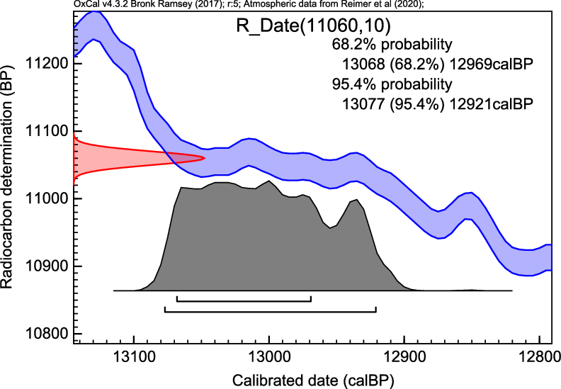
An important time anchor for the last glacial boundary is the Laacher See eruption in Germany. The 14C date for this eruption has been established as 11,060 ± 10 BP (1-σ, Kromer et al. Reference Kromer, Friedrich, Hughen, Kaiser, Remmele, Schaub and Talamo2004). This corresponds to a calibrated range of 12,850–13,050 calBP (95.4% confidence or 2-σ) using IntCal13. Note that, due to the plateau in the calibration curve that exists at the start of the YD, the high precision seen in the 14C 14C date (in BP) is not converted into a precise calendar age estimate. However, we can say that using IntCal20 will move this anchor date more into the B/A, and away from the YD boundary with a calibrated range of 12,920–13,080 calBP (95.4% confidence or 2-σ, see Figure 1). The 14C date is calibrated using OxCal v.4.3.2 (Bronk Ramsey Reference Bronk Ramsey2009b) using the new IntCal20 calibration curve. We have rounded the calibrated result to 10 calBP.

Figure 1 Calibrating the Laacher See tephra horizon.
The Minoan Santorini (Thera) Eruption
For calibration purposes, chronological anchor points provide crucial tests. A case in point of major importance is the catastrophic Minoan eruption of the Santorini/Thera volcano in the second millennium BC, a crucial anchor for Bronze Age prehistory. The precise date of the eruption has been debated for decades. Using a Greenland ice core chronology, the Thera eruption was originally thought to date to around 1645 BC based upon volcanic tephra found in the core. However, a recent and timely analysis shows that these volcanic horizons are more likely to be the result of eruptions in Alaska rather than Thera (McAneney and Baillie Reference McAneney and Baillie2019). 14C dating obviously plays a major role in this discussion. The debate has been and still is that 14C shows older dates than archaeological dating of the eruption, up to more than a century. For a recent overview of this debate, see Antiquity (2014).
Summarized, the 14C date of the eruption can be taken as 3350 ± 10 BP (1-σ), which is an average of many dates from key sites like Palaikastro and Akrotiri (Bronk Ramsey et al. Reference Bronk Ramsey, Manning and Galimberti2004; Bruins et al. Reference Bruins, MacGillivray, Synolakis, Benjamini, Keller, Kisch, Klugel and van der Plicht2008). This number (the 14C date) is confirmed by other analyses (Höflmayer Reference Höflmayer2012) and consistent with other records like tsunami deposits on Crete (Bruins et al. Reference Bruins, MacGillivray, Synolakis, Benjamini, Keller, Kisch, Klugel and van der Plicht2008). Calibrating this 14C date with calibration curves prior to the present IntCal20 curve yields a calendar date of the event in the late 17th century BC, most notably by wiggle matched 14C dates of tree rings from an olive tree killed by the eruption. This resulted in a date of 1627–1600 BC for the event (Friedrich et al. Reference Friedrich, Kromer, Friedrich, Heinemeier, Pfeiffer and Talamo2006), between 100–150 years older than previous traditional archaeological assessments.
This difference between archaeology and 14C has spawned debates lasting decades (Kutschera et al. Reference Kutschera, Bietak, Wild, Bronk Ramsey, Dee, Golser, Kopetzky, Stadler, Steier and Thanheiser2012; Antiquity 2014; Manning Reference Manning2014; Bruins and van der Plicht Reference Bruins and van der Plicht2017). Thus far, the debate has been largely focused on possible errors on either side, 14C, or archaeology. However, there is also the option that both are correct (or at least not very wrong), rather that there is a problem with the connection between the two: that is the calibration, which translates BP dates into calendar ages.
Very recently, new insights on the matter have been revealed. First, the validity of olive trees for wiggle match dating was questioned (Ehrlich et al. Reference Ehrlich, Regev and Boaretto2018). This is not further discussed here. Second, a new single year calibration curve for the Minoan Santorini time range became available, showing the possibility of an early 16th century BC date for the eruption (Pearson et al. Reference Pearson, Brewer, Brown, Heaton, Hodgins, Jull, Lange and Salzer2018). Note that a small wiggle in the calibration curve around 1570 BC (3520 calBP) is just missed by previously released curves. If a 14C age happens to coincide with this wiggle then it opens up an additional potential calendar age fit at this time and hence increases the probability of a younger (more recent) calendar date for the eruption.
This development led to major 14C (re)dating efforts of wood dated by dendrochronology for the relevant time range. Several laboratories measured single year rings with ultimate precision during the construction time of IntCal20. The datasets are reported in this issue (Friedrich et al. Reference Friedrich, Kromer, Wacker, Olsen, Remmele, Lindauer, Land and Pearson2020; Kuitems et al. Reference Kuitems, van der Plicht and Jansma2020). As a result, the “Thera time-range” presently has the best-dated calibration curve, with over 800 high-precision measurements on dendrochronologically dated wood between 1700 and 1500 calBC, obtained by several independent AMS laboratories.
The result is that indeed between ca. 3600 and 3500 calBP the calibration curve needs a shift of about 20 BP upwards in 14C age, as can be seen in Figure 2. By itself, this confirms the original observation by Pearson et al. (Reference Pearson, Wacker, Bayliss, Brown, Salzer, Brewer, Bollhalder, Boswijk and Hodgins2018) and so, after calibration, the calendar dates will, therefore, become younger by a certain amount. What does this mean in practice for the calendar date of the Minoan Santorini/Thera eruption? We will illustrate this as follows:

Figure 2 The IntCal20 (red) and IntCal13 (blue) calibration curves for the time range relevant to the Thera eruption. The thick lines represent the posterior mean of each curve; the thin lines represent the 1-σ credible/predictive interval. (Please see electronic version for color figures.)
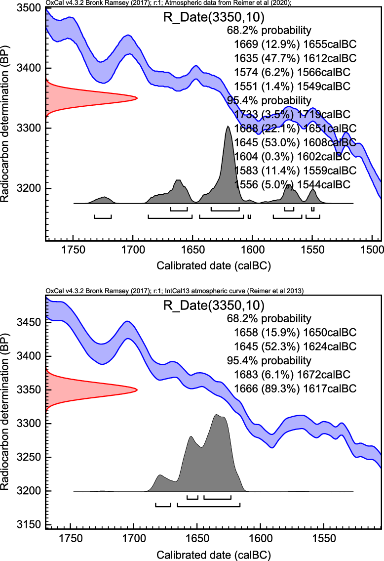
First, we calibrate the well-published averaged date 3350 ± 10 BP (1-σ) using both curves; see Figure 3. Note that the calibrated dates are shown here in BC.

Figure 3 Calibration of the averaged Thera date 3350 ± 10 BP, using IntCal20 (top) and IntCal13 (bottom).
This example highlights that near plateaus in the calibration curve, or during periods of significant wiggles, it is highly likely that calibrated age estimates arising from single 14C determinations will exhibit significant multimodality. In the presence of such multimodality, practical interpretation of dating is more complex and it is critical that care is taken to provide such interpretation correctly. Reporting single 68.2% (1-σ), or 95.4% (2-σ), intervals will typically be inappropriate and we instead recommend considering HPD regions.
With IntCal13, the posterior calendar age estimate is approximately unimodal (i.e. shows a single large peak). In such an instance, it is reasonable to report a single interval—here we obtain a 68.2% (1-σ) interval extending from 1658–1624 calBC; and a 95.4% (2-σ) interval of 1683–1617 calBC.
However, with IntCal20 the picture is much more complex as our 14C date of 3350 ± 10 BP hits the plateau in the curve. There are now multiple, disjoint, calendar age ranges consistent with this 14C date. A single interval is not therefore sufficient to summarize these possibilities. Instead, we see that there are perhaps five separate calendar age regions each with significant probabilities attached. In providing interpretation, we would suggest reporting all these regions with their associated probabilities.
If, for IntCal20, we want to provide the equivalent of a 2-σ interval (i.e. the smallest set of calendar ages which contains the true age with a probability of 95.4%), then should report the HPD region. This consists of all the intervals quoted in the 95.4% OxCal summary i.e. 1733–1719, 1688–1651, 1645–1608, 1604–1602, 1583–1559, and 1556–1544 calBC. The individual probabilities for these ranges are 3.5, 22.1, 53.0, 0.3, 11.4, and 5% respectively. The latter two, representing calendar dates in the 16th century BC, have a combined probability of 16.4%. A more recent date is, therefore, a distinct possibility, although we note that the peak centered around 1625 calBC carries the largest individual probability. We also note that a further small peak at an older age of ca. 1665 calBC appears, introduced by the refined revision, and increased wiggliness, of the new curve.
We further calculated the probability of a calendar date more recent than 1600 calBC (equivalently 3550 calBP) by summing the individual posterior probabilities of all calendar ages in that period. This provided an estimated probability of 19.3% for a calendar date in the 16th century BC.
Second, we reanalyze the wiggle match date of the olive branch published by Friedrich et al. (Reference Friedrich, Kromer, Friedrich, Heinemeier, Pfeiffer and Talamo2006). In the original publication, the actual calibration curve at the time was IntCal04. Subsequent calibration curves (IntCal09, IntCal13) did not significantly change the results. What will change using IntCal20?
The results of wiggle matching the olive tree dates are shown in Figure 4. For completeness we give here the four 14C dates of Friedrich et al. (Reference Friedrich, Kromer, Friedrich, Heinemeier, Pfeiffer and Talamo2006), measured by radiometry in Heidelberg: rings 1–13, 3383 ± 11 BP; rings 14–37, 3372 ± 12 BP; rings 38–59, 3349 ± 12 BP; rings 60–72, 3331 ± 10 BP (all at 1-σ).

Figure 4 Dating the Minoan Thera eruption (Friedrich et al. Reference Friedrich, Kromer, Friedrich, Heinemeier, Pfeiffer and Talamo2006) by wiggle matching rings from an olive tree branch, using the calibration curves IntCal20 (top) and IntCal13 (bottom).
For IntCal20, we see that through wiggle matching, multimodality in the calendar age estimate is reduced. This is typically to be expected since, when wiggle matching, we can use the shape of the curve in addition to its absolute value. The resulting calendar dates for the last ring are 1612–1592 calBC (68.2% confidence) and 1617–1578 calBC (95.4% confidence). For IntCal13, this is 1619–1608 calBC (68.2% confidence) and 1625–1604 calBC (95.4% confidence).
However, even here, we need to be somewhat careful with our interpretation as the IntCal20 estimate still retains two distinct peaks suggesting the two most likely periods for the last ring are either ca. 1605 calBC (3555 calBP) or ca. 1595 calBC (3545 calBP). Both these IntCal20-based potential calendar dates are more recent than the calendar age estimate obtained using IntCal13 (or earlier curves) by about 5–15 years showing the effect of the calibration curve change assuming the validity of the olive wood wiggle match.
Summarizing, for the Minoan Santorini/Thera eruption, we have with IntCal20 a relatively small revision to the curve itself which nonetheless has a significant impact not only in the calibrated ages it provides but also in how those age estimates may need to be reported and interpreted. Until IntCal20, the calibration curve in this time range was based on relatively sparse data (conventional dates measured decades ago, with relatively large temporal resolution). Now we have obtained by way of an unprecedented effort a firm establishment of the calibration curve during one of the most important prehistoric chronological anchorpoints.
However, in terms of establishing the exact date of Thera, the new calibration curve interestingly still leaves questions unanswered due to the presence of the plateau in IntCal20 during the contested time period. To gain more precise insight into the timing using 14C, modeling of multiple 14C dates will likely be needed. The 14C dates are calibrated using OxCal v.4.3.2 (Bronk Ramsey Reference Bronk Ramsey2009b) with a 1-year resolution.
The Middle and Upper Paleolithic Period
Chronological studies suggest that Neanderthals disappeared approximately between 39 and 41 ka ago, which implies that they overlapped with Archaic Homo Sapiens for at least 2600 years and up to 5400 years (Higham et al. Reference Higham, Douka, Wood, Ramsey, Brock, Basell, Camps, Arrizabalaga, Baena and Barroso-Ruiz2014). Additional evidence for the co-existence of these two human species is represented by DNA data obtained from the analysis of an Archaic Homo Sapiens (37–42 ka calBP) from Romania, showing that between 6 and 9% of the genomic sequence of this individual was derived from Neanderthals (Fu et al. Reference Fu, Hajdinjak, Moldovan, Constantin, Mallick, Skoglund, Patterson, Rohland, Lazaridis and Nickel2015).
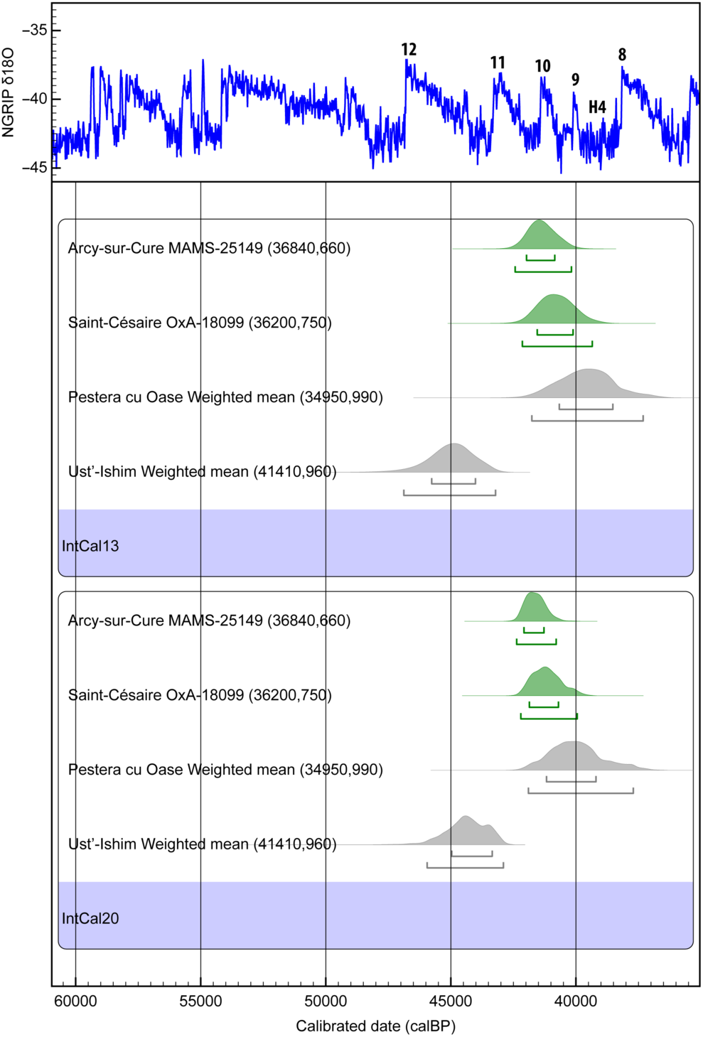
Despite the present state of the research, there remains still much to understand on the chronology of the Middle-to-Upper Paleolithic transition, i.e. on the period during which Archaic Homo Sapiens replaced Neanderthals in Eurasia, in order to construct a fairly convincing outline sketch of human prehistory and of the context in which it played out. Here, very precise and accurate calibration of 14C ages, back to ca. 50,000 years ago, is critical to limit archaeological speculations, developing solid chronologies of paleoenvironmental change and a more detailed understanding of the succession of climatic events through the last glacial period. In this paper, we will show what implications the new IntCal20 has for the understanding of the relationship between these two fascinating species using some of the most striking direct dates of human fossils in Eurasia. All the 14C dates are calibrated using OxCal v.4.3.2 (Bronk Ramsey Reference Bronk Ramsey2009b), and using both IntCal13 and the new IntCal20 calibration curve (Figure 5). The Figure 5 also shows part of the Greenland ice chronology (Rasmussen et al. Reference Rasmussen, Bigler, Blockley, Blunier, Buchardt, Clausen, Cvijanovic, Dahl-Jensen, Johnsen and Fischer2014). There are scale differences, but at this time range, the offsets are not significant beyond the 1-σ level. See Adolphi et al. (Reference Adolphi, Bronk Ramsey, Erhardt, Lawrence Edwards, Cheng, Turney, Cooper, Svensson, Rasmussen and Fischer2018) and also Muscheler et al. (Reference Muscheler, Adolphi, Heaton, Bronk Ramsey, Svensson, van der Plicht and Reimer2020 in this issue). All the results are rounded by 10 years.

Figure 5 The calibrated 14C ages using IntCal13 of Oase 1 and Ust’-Ishim are shown in grey, and Arcy-sur-Cure and Saint Césaire in green on top. The corresponding calendar age intervals using IntCal20 are shown at the bottom. The results are linked with the (NGRIP) δ18O climate record. The numbers from 12 to 8 represent the warm Dansgaard-Oeschger (DO events 12 to 8), and one cold Heinrich Event (H4).
Oase 1 and Ust’-Ishim
A Homo sapiens mandible (Oase 1) found in Romania (Peştera cu Oase) has been directly dated in the Oxford and Groningen laboratories yielding a mean age of 34,950 ± 990 BP (1-σ, Trinkaus et al. Reference Trinkaus, Moldovan, Milota, Bîlgar, Sarcina, Athreya, Bailey, Rodrigo, Mircea and Higham2003). The IntCal13 calibration places the Oase 1 individual at 40,670–38,520 calBP at 68.2% confidence, and at 41,770–37,310 calBP at 95.4% confidence.
This calibration provides evidence for an early Homo sapiens in Europe. Moreover, the genetic study found out that the Neanderthal-like DNA shares more alleles (between 6–9%) with the Oase 1 individual than it does with any present-day humans in Eurasia. They also estimated how far in time this introgression happened. They concluded that the Neanderthal contribution to the Oase 1 individual occurred recently in his family tree, four to six generations back, which means the Neanderthal admixture is dated less than 200 years before the time Oase 1 lived (Fu et al. Reference Fu, Hajdinjak, Moldovan, Constantin, Mallick, Skoglund, Patterson, Rohland, Lazaridis and Nickel2015).
The recalibration with IntCal20 provides a new time span for this important human fossil, placing his calendar age back in time, between 41,180–39,190 calBP at 68.2% confidence, and at 41,900–37,700 calBP at 95.4% confidence (see Figure 5). This shift to older ages of the presence of Homo sapiens at the site implies a longer overlap with Neanderthals in this region.
Another directly dated key human fossil was found in Siberia (Ust’-Ishim). In this case, it is the oldest Homo sapiens so far found in Eurasia (Fu et al. Reference Fu, Li, Moorjani, Jay, Slepchenko, Bondarev, Johnson, Aximu-Petri, Prufer and de Filippo2014). This individual carries a similar amount of Neanderthal DNA ancestry as present-day Eurasians. In this case, the Neanderthals gene flow occurred 7000 to 13,000 years before Ust’-Ishim lived. Here two dates were made in Oxford using the ultrafiltration method: OxA-25516 with a 14C Age of 41,400 ± 1300 BP (1-σ) and the second OxA-30190 with a 14C Age of 41,400 ± 1400 BP (1-σ). Applying R_Combine in OxCal we obtain an age of 41,400 ± 953 (1-σ). Calibrating against IntCal13, this corresponds to a calendar age of 45,770–44,010 calBP at 68.2% and 46,880–43,210 calBP at 95.4% (see Figure 5). With this result, the authors concluded that: interestingly the Ust’-Ishim individual probably lived during a warm Dansgaard-Oeschger period (DO 12) (Fu et al. Reference Fu, Li, Moorjani, Jay, Slepchenko, Bondarev, Johnson, Aximu-Petri, Prufer and de Filippo2014), which has been proposed to be a time of expansion of Homo sapiens into Europe (Müller et al. Reference Müller, Pross, Tzedakis, Gamble, Kotthoff, Schmiedl, Wulf and Christanis2011; Hublin Reference Hublin2012).
With the new calibration curve IntCal20, these ranges changes to 44,970–43,340 calBP at 68.2% and 45,950–42,890 calBP at 95.4%. This shift to younger ages puts the Ust’-Ishim individual closer or even into the stadial following DO 12 (see Figure 5).
The Châtelperronian
Another two, directly dated, important hominins are Neanderthals from France. The first is the Neanderthal fossil of Saint Césaire (La Roche-à-Pierrot) situated in the Charente-Maritime department of southwestern France (Lévêque and Vandermeersch Reference Lévêque and Vandermeersch1980). The second one comes from Grotte du Renne (Arcy-sur-Cure) located on the main road between Auxerre and Avallon, close to Paris (David et al. Reference David, Connet, Girard, Lhomme, Miskovsky and Roblin-Jouve2001). Both of them are crucial to understanding the replacement processes of Neanderthals by Homo sapiens and the interpretation of so-called “transitional industries”, here the Châtelperronian.
The question of whether Neanderthals manufactured the Châtelperronian is the topic of intense debate since the Châtelperronian industry represents a new cultural behavior. The debated question is if the Châtelperronian new behavior demonstrates a cultural influence, on the last Neanderthals, by contemporaneous Archaic Homo Sapiens populations, already present further east in Europe, or if it represents a Neanderthal invention. Here, direct 14C dates of hominins together with a precise calibration curve play a pivotal role.
The Saint Césaire bone was pretreated at the Max Planck Institue, Leipzig, Germany, and graphitized and dated in Oxford to a 14C age of 36,200 ± 750 (OxA-18099, 1-σ) (Hublin et al. Reference Hublin, Talamo, Julien, David, Connet, Bodu, Vandermeersch and Richards2012). The Arcy-sur-Cure bone was pretreated at the Max Planck and graphitized and dated in Mannheim, Germany to a 14C age 36,840 ± 660 (MAMS-25149, 1-σ) (Welker et al. Reference Welker, Hajdinjak, Talamo, Jaouen, Dannemann, David, Julien, Meyer, Kelso and Barnes2016). The respective calibrated ages using IntCal13 are 41,550–40,110 calBP at 68.2% and 42,150–39,340 calBP at 95.4% for Saint Césaire, and 41,980–40,840 calBP at 68.2% and 42,430–40,180 calBP at 95.4% for Arcy-sur-Cure (Figure 5).
IntCal20 provides a new calibration for Saint Césaire between 41,860–40,690 calBP at 68.2% and 42,200–39,940 calBP at 95.4%. For Arcy-sur-Cure the ranges are between 42,080–41,270 calBP at 68.2% and 42,370–40,780 calBP (Figure 5).
Conclusion
These examples demonstrate that for some intervals, here 40 ka calBP vs. 45 ka calBP, the new calibration curve will result in narrower ranges for calibrated ages i.e. more precise dating than the previous IntCal13. The more detailed IntCal20 calibration curve will, therefore, allow higher precision for the study of human evolution in terms of chronological overlap between archaeological sites and different human species and will provide better resolution in relation to climatic events.
Regional and Seasonal Effects
A full discussion of possible regional effects with associated references is given in the main IntCal20 paper (Reimer et al. Reference Reimer, Austin, Bard, Bayliss, Blackwell, Bronk Ramsey, Butzin, Edwards, Friedrich and Grootes2020 in this issue). The conclusion drawn there is that there is as yet insufficient information to quantify such effects or indeed to fully understand the contribution from different underlying mechanisms. The potential issues are: different growing seasons for the material dated compared to the calibration datasets, localized addition of CO2 from different reservoirs (such as ocean upwelling, anthropogenic sources, and local volcanic vents), mixture of air masses from both hemispheres in the tropics (Hogg et al. Reference Hogg, Heaton, Hua, Bayliss, Blackwell, Boswijk, Ramsey, Palmer, Petchey and Reimer2020 in this issue), and overall trends with latitude or altitude. Some of these effects are potentially related because the known subannual cycle in 14C (Appenzeller et al. Reference Appenzeller, Holton and Rosenlof1996; Stohl et al. Reference Stohl, Bonasoni, Cristofanelli, Collins, Feichter, Frank, Forster, Gerasopoulos, Gäggeler and James2003) will necessarily lead to differences in the 14C signal seen in different species and different latitudes. Furthermore, even the same species may grow differently due to circumstances such as water availability and other localized stresses. Fortunately, with the exception of the major addition of carbon from other reservoirs, most seasonal or regional effects are likely to be less than 20 14C years or 2.5‰ and so comparable to the measurement precision.
In considering the practical consequences of such regional and seasonal effects, statistically, we can treat measurements which are systematically offset irrespective of the underlying cause. This is particularly important where complex Bayesian models or wiggle-matching of tree ring data is being undertaken to achieve precisions approaching the decadal level. In these cases, it is prudent to build into the model the possibility that all of the 14C dates might be systematically offset by some small amount, whether this is due to an offset resulting from the measurement methodology, or within the sample itself relative to the hemispherical average atmosphere. Particularly in the case of wiggle-matched tree ring data, the measurement series itself will often provide sufficient evidence for whether there is such an offset. In general, it is better to provide a prior which reflects our expectation that such offsets will be small (for example, N(μ,σ2) ~ N(0,102)). This can be achieved, for example, in OxCal (Bronk Ramsey Reference Bronk Ramsey2009a) by using the Delta_R methodology normally applied to marine samples (as was used as a sensitivity test in Bronk Ramsey et al. Reference Bronk Ramsey, Dee, Rowland, Higham, Harris, Brock, Quiles, Wild, Marcus and Shortland2010). The code for this is:
Delta_R(“offset”,0,10);
or
Delta_R(“offset”,N(0,10));
Such an approach can also be used for single calibrations by adding in additional error in quadrature to reflect such uncertainty. However, before doing this, one should know whether this uncertainty has already been included within the error quoted by the laboratory. The overall effect on large datasets is likely to be much more significant in that any offsets are potentially correlated across the dataset as a whole, something which the lab cannot quantify (unless it is purely a measurement issue). It is important to remember that there is ultimately an irreducible uncertainty in our chronologies, irrespective of the number of measurements we make.
If one wishes to use the data to determine such an offset with no bias, a uniform prior (for example ~U(-20,20)) for the offset can be used, and the marginal posterior for the offset determined as part of the analysis. The OxCal code for this would be:
Delta_R(“offset”,U(-20,20));
The treatment of samples that come from close to the ITCZ is slightly different. Here we know the direction of the offset which we expect to see from whichever hemisphere we think is dominant. In such cases, it would be possible to use a mixed reservoir model, where we assume that the 14C could be drawn from a mixture of the northern and southern hemisphere atmospheric reservoirs. An alternative is to use the same approach as above but with a biased offset. In practice, for example, using the Northern Hemisphere curve with an offset of ~U(0,40) will give a similar result to using the Southern Hemisphere curve with an offset of ~U(-40,0). The difficulty in doing this is putting a more constrained prior on the expected mixture, which will be very location dependent; the above uniform distributions are very conservative but obviously add in significant extra uncertainty unless the dataset includes some samples of known age which will constrain the marginal posterior for the offset. Such situations are potentially very complex in that different samples, particularly if from different species, might pick up different signals even in the same location because of growing season changes in the ITCZ.
The Marine Curve
The slow diffusion of CO2 into and out of the surface ocean combined with the very slow circulation of the deep ocean results in a 14C age offset or reservoir effect (R(t)) between samples that lived on land and those that lived at the same time in the ocean. The present day value of this offset is of the order of approximately 400 14C yr; however, R(t) varies regionally and is time dependent. For sample 14C calibration of marine-based determinations, the regional variation has usually been handled by including a regional correction to the marine calibration curve called ΔR but the time dependence of both R and ΔR has made marine calibration more uncertain than for terrestrial samples.
The Marine20 curve (Heaton et al. Reference Heaton, Köhler, Butzin, Bard, Reimer, Austin, Ramsey, Grootes, Hughen and Reimer2020b in this issue) includes a global R(t) correction based on the BICYCLE box model (Köhler and Fischer Reference Köhler and Fischer2004, Reference Köhler and Fischer2006; Köhler et al. Reference Köhler, Fischer, Munhoven and Zeebe2005, Reference Köhler, Muscheler and Fischer2006) forced by our IntCal20 estimate of atmospheric 14C along with several other paleoclimate records. While more complex ocean general circulation models (OGCMs) are available (e.g. Butzin et al. Reference Butzin, Köhler and Lohmann2017, Reference Butzin, Heaton, Köhler and Lohmann2020 in this issue) which also provide spatial estimates for the marine 14C reservoir, most archaeological marine samples derive from near coastal environments which are not well characterized by the grid size of such OGCMs. Consequently, the use of ΔR with Marine20 can still be advised for these samples. Pre-bomb ΔR values have been recalculated with Marine20 and are available at www.calib.org/marine20. Researchers calibrating marine 14C ages from the open ocean sites may want to access the LSG OGCM model results (Butzin et al. Reference Butzin, Heaton, Köhler and Lohmann2020 in this issue) within the grid closest to the sample site available at https://doi.pangaea.de/. This is not discussed further here, for more details we refer to Heaton et al. (Reference Heaton, Köhler, Butzin, Bard, Reimer, Austin, Ramsey, Grootes, Hughen and Reimer2020b in this issue).
NOTE ON TIMESCALES
For completeness, we summarize here the units and definitions for timescales that are relevant for 14C dating.
BP
Defined unit for the 14C timescale. Measured activities are to be reported following a convention. The definition concerns the usage of the halflife value, fractionation correction, and standard activity. For details, we refer to the literature (Stuiver and Polach Reference Stuiver and Polach1977; Mook and van der Plicht Reference Mook and van der Plicht1999).
AD
Anno Domini, calendar date as commonly used in western society.AD is the same as CE (Common Era) which is mostly used in Near Eastern contexts.
calAD
Calendar date, obtained after calibration of a 14C date (expressed in BP).
BC
Calendar date before (the birth of) Christ, which is traditionally placed in 1 AD. BC is the same as BCE (Before Common Era).The year “0” does not exist in the traditional calendar; the year 1 BC precedes 1 AD.
calBC
Calendar date, obtained after calibration of a 14C date (expressed in BP).
calBP
Calibrated 14C date, relative to the standard year 1950 AD.Thus, calBP = 1950 – calAD = 1949 + calBC.
Note one exception to the above: modeled dates are given as BP. After applying Bayesian analysis of a series of 14C dates only, this equals calBP. The latter is no longer the case when also dates resulting from other methods are included.
b2k
Calendar date relative to 2000 AD. This unit is not to be used for 14C dating. We mention it here because it has recently been introduced by the ice core community to avoid confusion with “our” calBP (Rasmussen et al. Reference Rasmussen, Bigler, Blockley, Blunier, Buchardt, Clausen, Cvijanovic, Dahl-Jensen, Johnsen and Fischer2014). The units BP and calBP are both used in e.g. Earth and Environmental sciences when dating methods other than 14C are used. However, generally, they have a different meaning than the 14C definitions given above. We should be aware that BP and calBP are not “owned” by the radiocarbon community.
CONCLUSIONS
The calibration curve to be used for calibration of 14C dates has been updated. It is presently called IntCal20, to be used for terrestrial samples from the Northern Hemisphere. It replaces the previous curve IntCal13. Additional calibration curves associated with IntCal20 are Marine20 for samples from marine reservoirs, and SHCal20 for the Southern Hemisphere.
In this companion article, we have summarized the present status of calibration and discuss some highlights. The full background of curve construction is briefly summarized in order to provide users with an understanding of the method used. Details and reference to datasets are given in the main papers in this issue.
As before, the calibration curve can be considered as based on two kinds of records: dendrochronology and others. The tree ring part now extends to 13,910 calBP, well into the Late Glacial period. Here the main improvement since IntCal13 is the temporal resolution. For significant parts of (pre)history, single-year datasets have become available. This is spawned by the hunt for “Miyake events”, sudden increases in the natural 14C content of short duration, observed in tree rings. Equally important, the newest MICADAS AMS machines are very efficient, enabling the acquisition of an unprecedented amount of tree-ring dates with high resolution. This has revolutionized the field, including calibration.
A key illustration concerns the dating of the Minoan Santorini/Thera eruption. This is a crucial anchor point for prehistory in the 2nd millennium BC. For decades, the absolute date of the eruption has been heavily debated by 14C experts and traditional archaeological thinking. During the last few years, many high-resolution tree-ring measurements have been performed by various laboratories, which are now all integrated into IntCal20. The revised curve in the relevant time period is now annually resolved and shifted by a relatively small but crucial number of years (ca. 20 BP). As a consequence of this shift, there is a plateau in the calibration curve with detailed annual fluctuations that provide multiple potential fits with 14C dates from the eruption. This has an impact not just in shifting calendar age estimates more recent, but also results in multimodal calendar age estimates that require significant care in interpretation. A much younger date—ca. 1500 BC, as advertised by some archaeologists—remains extremely unlikely, based on 14C.
For the Glacial part of the curve, beyond the tree ring record of 13,910 calBP, the main datasets originate from corals, speleothems, and the laminated sediment of Lake Suigetsu. The new IntCal20 integrated curve provides calibration back to 50,000 BP, which corresponds to 55,000 calBP. This part of the curve is applied to critical real-life chronological issues in Paleolithic archaeology. We discuss the absolute dates for the key Paleolithic sites Pestera Cu Oase (Romania), Ust’-Ishim (Siberia), Arcy-sur-Cure, and Saint Cesaire (France). We show that the more detailed IntCal20 calibration curve allows better precision for the study of human evolution in terms of chronological overlap between the presence of Homo sapiens and Neanderthals. It also provides better resolution in relation to climatic events.
ACKNOWLEDGMENTS
CBR is funded by NERC as part of their 14C facility. TJH is funded by a Leverhulme Trust Fellowship RF-2019-140\9, “Improving the Measurement of Time Using Radiocarbon”. ST is funded by the European Research Council under the European Unionʼs Horizon 2020 Research and Innovation Programme (grant agreement No. 803147-RESOLUTION). Discussions with M.W. Dee have been instrumental.


 Open access