


INTRODUCTION
Records of deglaciation are critical to understanding the response of ice sheets to a warming climate and changing sea level, and they are essential for constraining models of changing climate (e.g., Clark et al., Reference Clark, Dyke, Shakun, Carlson, Clark, Wohlfarth, Mitrovica, Hostetler and McCabe2009; Vieli and Nick, Reference Vieli and Nick2011; Seguinot et al., Reference Seguinot, Khroulev, Rogozhina, Stroeven and Zhang2014, Reference Seguinot, Rogozhina, Stroeven, Margold and Kleman2016). They are also needed for speculation on the routes and timing of human migration into the Americas (e.g., Mandryk et al., Reference Mandryk, Josenhans, Fedje and Mathewes2001; Erlandson et al., Reference Erlandson, Torben, Braje, Casperson, Culleton, Fulfrost and Garcia2011). The Cordilleran Ice Sheet (CIS) overlaid the western margin of the coastal mountain ranges of Washington, British Columbia, Yukon, and southern Alaska, with numerous marine-terminating glaciers along the Pacific margin (Fig. 1). Recent refinements constrain the terrestrial deglaciation history of much of the CIS (e.g., Stroeven et al., Reference Stroeven, Fabel, Margold, Clague and Xu2014; Balbas et al., Reference Balbas, Barth, Clark, Clark, Caffee, O'Connor, Baker, Konrad and Bjornstad2017; Clague, Reference Clague2017; Kopczynski et al., Reference Kopczynski, Kelley, Lowell, Evenson and Applegate2017; Menounos et al., Reference Menounos, Goehring, Osborn, Margold, Ward, Bond and Clarke2017; Darvill et al., Reference Darvill, Menounos, Goehring, Lian and Caffee2018; Lesnek et al., Reference Lesnek, Briner, Baichtal and Lyles2020), but are lacking along the southern and southwestern Alaska margin.

Figure 1. Late Wisconsinan (approximately last glacial maximum) and Pleistocene maximum extent of glaciers in Alaska, modified from Kaufman et al. (Reference Kaufman, Young, Briner, Manley, Ehlers, Gibbard and Hughes2011). Inset map shows the position of these glaciers with respect to the Cordilleran Ice Sheet (CIS) and the Laurentide Ice Sheet (LIS) in North America (glacial extents from Batchelor et al., Reference Batchelor, Margold, Krapp, Murton, Dalton, Gibbard, Stokes, Murton and Manica2019). Note the asymmetry of late Wisconsinan glaciers on the southern Alaska margin, with glaciers covering almost the entire landscape in contrast to the north side of the Alaska Range and Alaska Peninsula, which had short glaciers, due to rain shadow effects. Modern glaciers, in light blue, show the location of high topography. Inset box shows location of study area in Fig. 2A. Black dots with letter labels: A, Anchorage; K, Katalla; S, Sanak Island; W, Wingham Island. Location D refers to core EW0408 85JC discussed in Davies et al. (Reference Davies, Mix, Stoner, Addison, Jaeger, Finney and Wiest2011), and location CS refers to core EW0408 66JC offshore Cross Sound discussed in Praetorius and Mix (Reference Praetorius and Mix2014).
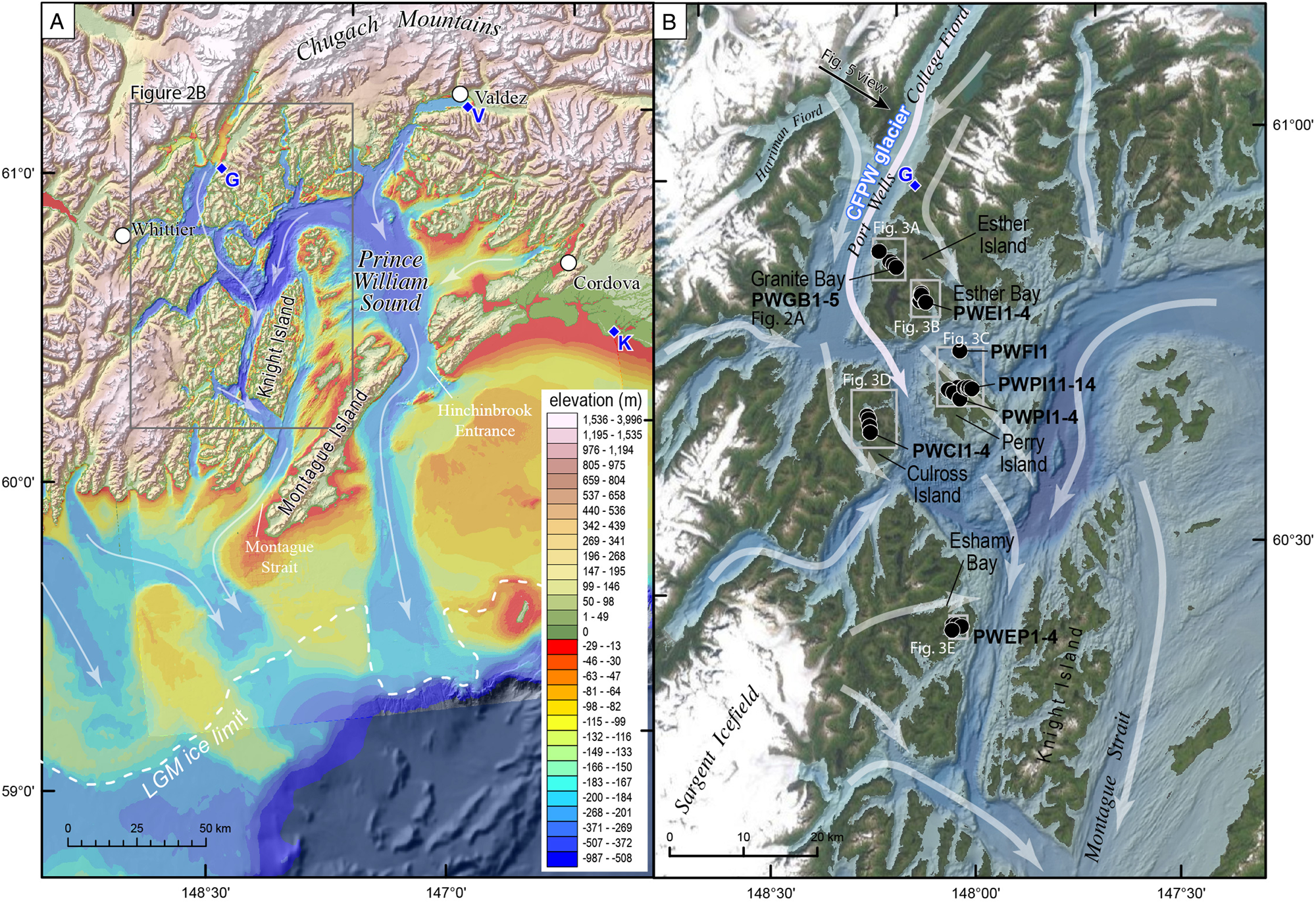
Figure 2. Geographic setting of the Prince William Sound (PWS) and cosmogenic radionuclide (CRN) sampling sites. (A) Overview of topography and bathymetry of PWS. White arrows show the flow direction of major glaciers and ice streams at last glacial maximum (LGM) time from Kaufman et al. (Reference Kaufman, Young, Briner, Manley, Ehlers, Gibbard and Hughes2011) with minor modifications from Haeussler et al. (Reference Haeussler, Armstrong, Liberty, Ferguson, Finn, Arkle and Pratt2015). Blue diamonds labeled G, V, and K are locations of prior 14C dates (see text and Table 1). G, Golden; V, Valdez; K, Katalla. Location of Fig. 2B is shown and labeled. (B) A more detailed view of northwestern PWS showing sampling areas and locations of site maps shown in Fig. 3. White arrows show inferred LGM glacial flow directions from aligned valleys and glacial striae. CFPW glacier is the College Fiord–Port Wells glacier that is inferred to have covered all of the sampling sites, except those sites in the area of Fig. 3E, which was covered by a glacier emanating from the Sargent Icefield.

Figure 3. Maps of sampling sites and cosmogenic ages, in kiloyears (Table 3, column with GIA correction). See Fig. 2B for locations within Prince William Sound. Background satellite image from Esri World Imagery compilation (https://services.arcgisonline.com/ArcGIS/rest/services/World_Imagery/MapServer/0, accessed 28 May 2021). (A) Sampling area near Granite Bay on Esther Island. We refer to this area as “Granite Bay” or “Granite Bay on Esther Island.” (B) Sampling area near Esther Bay on Esther Island. We refer to this area as “Esther Bay.” (C) We sampled the ridges on the east and west sides of East Twin Bay on Perry Island. We refer to these transects as “Perry-East” or “Perry-West.” In our summary plots, both transects share a sampling site (PWPI1) in the middle of the bay. Note the solitary Fool Island sample site lies to the north. (D) Sampling area near Hidden Bay on Culross Island. We refer to this sampling area as “Culross.” (E) This sampling area lies near Eshamy Bay, and we refer to this sampling transect as “Eshamy.”
Table 1. Basal radiocarbon ages in and near Prince William Sound, Alaska.
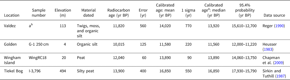
a All samples calibrated using OxCal v. 4.3.2 (Bronk Ramsey, Reference Bronk Ramsey2017) and IntCal13 (Reimer et al., Reference Reimer, Bard, Bayliss, Beck, Blackwell, Ramsey and Buck2013).
b Laboratory number GX-10789.
We examine the deglaciation of Prince William Sound (PWS), Alaska, which lies on the southern side of the northernmost extent of the CIS (Figs. 1 and 2). We aim to establish the history of deglaciation, compare it with other records from Alaska, and evaluate oceanographic and atmospheric linkages and drivers. Kaufman et al. (Reference Kaufman, Young, Briner, Manley, Ehlers, Gibbard and Hughes2011) showed the maximum limits of Pleistocene and late Wisconsinan glaciers in Alaska (Fig. 1). They state this is approximately equivalent to the last glacial maximum (LGM) at approximately 26 to 20 ka (Clark et al., Reference Clark, Dyke, Shakun, Carlson, Clark, Wohlfarth, Mitrovica, Hostetler and McCabe2009). Kaufman et al. (Reference Kaufman, Young, Briner, Manley, Ehlers, Gibbard and Hughes2011, p. 443) also noted, “Nowhere else in Alaska is the extent of Pleistocene glacier ice more poorly constrained than along the southern margin of the Cordilleran Ice Sheet.” Thus, the marine limits of these glaciers are estimated almost everywhere on the map (Fig. 1), and in general are inferred to have extended to the edge of the continental shelf, particularly where cross-shelf troughs exist. Minor modifications to these ice limits were inferred by Haeussler et al. (Reference Haeussler, Armstrong, Liberty, Ferguson, Finn, Arkle and Pratt2015) for a region offshore PWS and by Zimmerman et al. (Reference Zimmermann, Prescott and Haeussler2019) for a region offshore the Alaska Peninsula.
There are some recent constraints on the retreat history of marine-terminating ice for the region east of PWS. At a site on the upper continental slope (Fig. 1, location D), south of Kayak Island, Davies et al. (Reference Davies, Mix, Stoner, Addison, Jaeger, Finney and Wiest2011) interpreted a transition from coarse glacial-marine sediments to finely laminated sediments at 14,790 ± 380 cal yr BP as the time that tidewater glaciers to the north retreated onto land or behind fjord sills. Further southeast, west of Cross Sound (Fig. 1, location CS) and Glacier Bay, Praetorius and Mix (Reference Praetorius and Mix2014) infer significant landward retreat of glaciers between ~13 and 12.5 ka based on radiocarbon dating and changes in sediment type. Praetorius et al. (Reference Praetorius, Condron, Mix, Walczak, McKay and Du2020) also provide a paleo–sea surface temperature record for the North Pacific showing lower temperatures around 17 ka and warming until about 14.6 ka, which was followed by a cooling trend through the Younger Dryas, then followed by warming about 12.1 ka. These marine studies lead us to evaluate the deglaciation history in a region with less dramatic coastal topography and the relationships between the sea-surface temperature history on glacial thinning and retreat in PWS.
Only two radiocarbon ages from within PWS constrain the timing of glacial retreat soon after the LGM. One of these ages is from a sample collected near the town of Valdez (Fig. 2, location V), where a basal peat overlying till gave a 14C age of 14,020 ± 770 cal yr BP (Reger, Reference Reger1990; Table 1). This unique exposure was found during large excavations related to construction of an oil-transportation facility. Heusser (Reference Heusser1983) found and analyzed another basal peat in Port Wells (Fig. 2, location G), which has an age of 11,580 ± 220 cal yr BP (Table 1). Both localities are in northern PWS, far north of the shelf edge, and thus deglaciation of more distal regions likely began earlier than roughly 14,000 yr BP. More recent Neoglacial and Little Ice Age (LIA) and retreats of glaciers in the last 4 ka are well studied in PWS and adjacent areas (e.g., Wiles et al., Reference Wiles, Barclay and Calkin1999; Barclay et al., Reference Barclay, Wiles and Calkin2009), but not the late Quaternary deglaciation. As we could not date moraines, our approach to examining deglacial timing was through cosmogenic radionuclide (CRN) exposure dating of vertical profiles of glacially striated surfaces on islands that serve as “dipsticks” for the thickness of glaciers that were within PWS. This dipstick approach has been successfully used in a number of locations to quantify glacial thinning (e.g., Stone et al., Reference Stone, Balco, Sugden, Caffee, Sass, Cowdery and Siddoway2003; Mackintosh et al., Reference Mackintosh, White, Fink, Gore, Pickard and Fanning2007; Corbett et al., Reference Corbett, Bierman, Wright, Shakun, Davis, Goehring, Halsted, Koester, Caffee and Zimmerman2019).
GEOLOGIC AND GEOGRAPHIC SETTING
The rocks in PWS are part of a vast accretionary complex of Paleocene–Eocene age (e.g., Plafker et al., Reference Plafker, Moore, Winkler, Plafker and Berg1994). These dominantly metasedimentary rocks were intruded by granitic plutons during Paleocene to Eocene time; some mafic volcanic rocks are also present (Nelson et al., Reference Nelson, Dumoulin and Miller1985; Bradley et al., Reference Bradley, Kusky, Haeussler, Goldfarb, Miller, Dumoulin, Nelson and Karl2003). The rocks were subsequently exhumed in middle to late Cenozoic time (Arkle et al., Reference Arkle, Armstrong, Haeussler, Prior, Hartman, Sendziak and Brush2013; Ferguson et al., Reference Ferguson, Armstrong, Arkle and Haeussler2015), forming the present mountainous landscape. The region lies above the shallowly dipping Alaska–Aleutian subduction zone, which last ruptured in 1964 in a Mw9.2 earthquake (Plafker, Reference Plafker1969), which is the second largest earthquake ever recorded. Paleoseismological studies indicate earthquakes of similar magnitude occur on average every ~535 yr (Shennan et al., Reference Shennan, Bruhn, Barlow, Good and Hocking2014), causing strong ground shaking, landslides, and toppling of rocks and boulders. Today, and in the past (Kaufman et al., Reference Kaufman, Young, Briner, Manley, Ehlers, Gibbard and Hughes2011), there has been a strong asymmetry to the length of glaciers on either side of the Chugach and Kenai Mountains that flank PWS (see Fig. 1), because storm systems travel northeasterly from the Aleutians and have prevailing southerly winds (Shulski and Wendler, Reference Shulski and Wendler2007). Glaciers filled almost the entire landscape on the southern sides of the coastal mountains, in contrast to the northern sides, which had relatively short glaciers.
The physiography of the region is of a three-sided bowl, with high mountains on the north, east, and west sides, where glaciers still cover most of the landscape above ~700 m (Figs. 1 and 2). The highest peaks of the Chugach Mountains, with summits as high as 4016 m, lie at the northwestern edge of PWS. The central part of PWS has islands with rounded summits indicating glacial sculpting, presumably during the LGM. The bathymetry includes a series of troughs and shows that trunk glaciers exited PWS through Hinchinbrook Entrance and Montague Straight (Fig. 2). Kaufman and Manley (Reference Kaufman, Manley, Ehlers and Gibbard2004) and Kaufman et al. (Reference Kaufman, Young, Briner, Manley, Ehlers, Gibbard and Hughes2011) inferred that glaciers extended to the edge of the continental shelf at LGM time. The terrestrial Quaternary geology of PWS has never been studied in detail, and only bedrock geologic maps exist of the region (e.g., Nelson et al., Reference Nelson, Dumoulin and Miller1985). Late Quaternary and Holocene deposits consist of alluvial sand and gravel in valley bottoms, small LIA moraines, and colluvial deposits (e.g., Nelson et al., Reference Nelson, Dumoulin and Miller1985; Wiles et al., Reference Wiles, Barclay and Calkin1999). Bedrock bedding, faults, and fractures are clearly visible where not obscured by vegetation, showing the entire landscape was abraded by glaciers during glacial maxima. Finally, given glacial retreat, we assume there was glacial-isostatic adjustment (GIA). However, evidence for this uplift in the form of terraces or uplifted marine deposits has not been reported in the literature (see the compilation of Shugar et al., Reference Shugar, Walker, Lian, Eamer, Neudorf, McLaren and Fedje2014), and we have not seen such features.
SAMPLING STRATEGY, SITES, AND METHODS
To better understand the timing of glacial thinning and retreat in PWS, we sampled quartz-bearing granitic bedrock to date the exposure of glacially scoured surfaces using cosmogenic 10Be (Fig. 3). Using the typical cosmogenic exposure method to date boulders in moraines (e.g., Ivy-Ochs and Briner, Reference Ivy-Ochs and Briner2014) was not possible, because the terminal moraines are offshore and underwater, and no other LGM moraines are mapped to examine. For sampling scoured bedrock, we looked for locations with varying distances along paleo–ice streams and for locations where we could collect a suite of samples in a small area that would provide a vertical transect that might allow us to document the thinning of an ice sheet. We chose locations as far as practical from modern valley and alpine glaciers, so they would be unaffected by Neoglacial ice advances (Barclay et al., Reference Barclay, Wiles and Calkin2009), such as in the Harriman Fiord area (Fig. 2B). We also looked for locations with rounded summits, because this morphology implies that glaciers overran the surface. During our fieldwork, we examined numerous outcrops of both the metasedimentary and granitic rocks. Although we could find undulatory and scoured surfaces on metasedimentary rocks indicative of glacial scour, we were unable to find any clear glacial striae. The rocks were often highly weathered and fractured, indicating surface lowering since exposure, and poor in quartz, making them mediocre candidates for cosmogenic exposure dating. We exclusively sampled granitic rock, because it contains abundant quartz, and we targeted bedrock outcrops hosting well-preserved glacial scour features, grooves, polish, pluck marks, and striae (Fig. 4). Although bedrock outcrops can be susceptible to 10Be inheritance (e.g., Brook et al., Reference Brook, Kurz, Ackert, Denton, Brown, Raisbeck and Yiou1993; Ivy-Ochs and Briner, Reference Ivy-Ochs and Briner2014), we did not sample any boulders because (1) we found no exposed moraines; (2) erratics perched on bedrock often appeared toppled by frost jacking or earthquake shaking; and (3) erratics on mountaintops and ridges were either nonexistent or rare. We sampled five main sites on three islands and a mainland peninsula (Figs. 2 and 3). Most samples came from broad ridges that lacked soils, had little vegetation, and minimized topographic shielding. This study was limited by the lack of paired boulder and bedrock samples, and we were unable to directly test for cosmogenic inheritance.
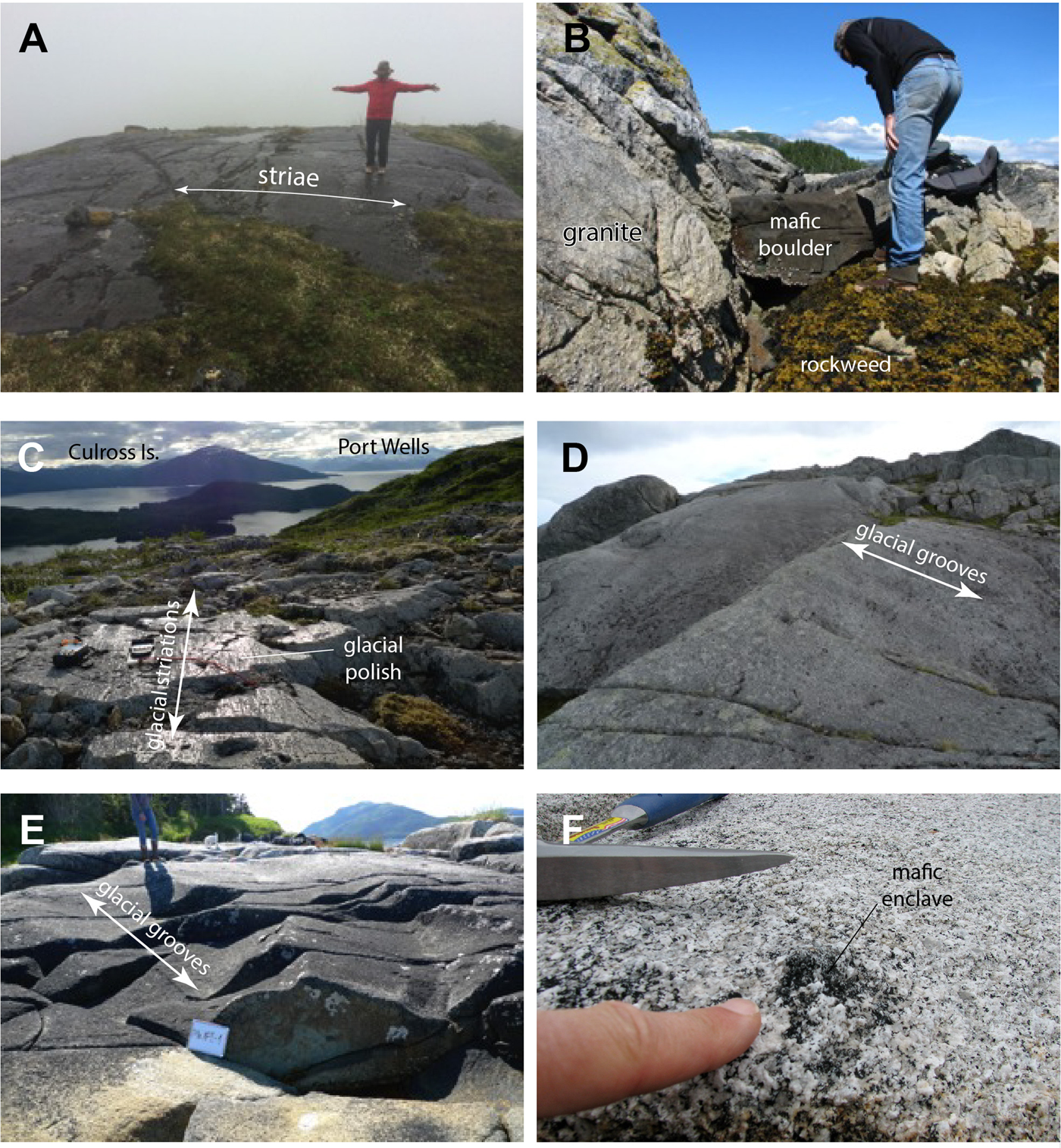
Figure 4. Glacial features at sampling sites. All photographs by PJH, U.S. Geological Survey. (A) Smooth scoured and striated surface above Esther Bay, on Esther Island at site PWEI1, which is located at a pass (see Fig. 3B). Person is holding their arms parallel to the striae. (B) At sea-level elevation, sample site PWPI1 in East Twin Bay on Perry Island (see Fig. 3C). Person is standing on rockweed (Fucus distichus), which grows up to approximately mean high tide level. Left of the person's leg is a mafic boulder; the closest outcrop of this rock type occurs 25 km to the southeast. We infer the boulder must have been ice rafted to the present location. (C) At the rounded summit of Perry Island at site PWPI4 (Fig. 3C), showing glacial polish and striae, which point toward ice overtopping this island and coming from the direction of Port Wells. (D) Glacial striae and grooves near the summit of Culross Island near site PWCI4. (E) Glacial grooves and plucked faces from Fool Island (Fig. 3C). (F) Typical expression of 1–3 mm of positive relief of a mafic enclave. This shows that surface lowering of the granites is inconsequential for the cosmogenic ages.
Tidewater glaciers remain in northern and western PWS, and at LGM time these glaciers would have overrun the sampling localities (Fig. 2). Glacial striations, grooves, roche moutonnée, and drainage patterns indicate that a large trunk glacier, which we refer to as the “CFPW Glacier,” flowed down College Fiord and Port Wells and overran Esther, Culross, and Perry Islands (Fig. 2B). This glacier, which may have been an ice stream, flowed toward central PWS and ultimately exited the sound through Montague Strait (Fig. 2). We observed stranded hanging glacial troughs north of Esther Island, parallel to College Fiord and Port Wells (Fig. 5). These U-shaped troughs are oriented north-northwesterly and indicate the margins of the CFPW glacier once blanketed the mountains on the east side of the fjord. It is reasonable to assume this same large CFPW glacier overran Esther Island, producing its rounded summits. Farther south, the CFPW glacier overran Culross and Perry Islands with their rounded summits. Glacial striae on the summits of Perry and Culross Islands point toward Port Wells and are consistent with this inferred ice flow direction (Fig. 4C and D). The one sampling locality that did not have the CFPW glacier as its source is near Eshamy Bay. This locality had ice sourced from the nearby Sargent Ice Field that lies 20 km to the west (see Figs. 2B and 3D). Eshamy Bay is a U-shaped, east-west trending valley, with a broad U-shaped saddle at its western end. This geomorphology demonstrates eastward ice flow from the Sargent Ice Field down the bay and over the sampling locality. Given the proximity of this site to the modern Sargent Icefield, this site was closer to the paleo–ice source than any of the others.
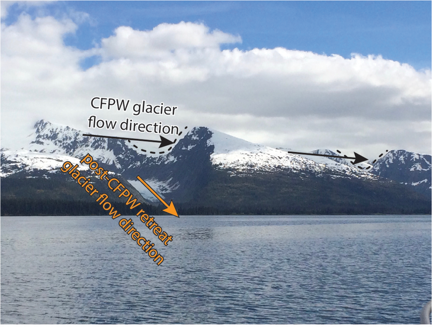
Figure 5. Abandoned hanging glacial valleys, outlined by dashed lines, to the north-northwest of Esther Island near Coghill Lake (location on Fig. 2B). The black lines and arrows show the south-southeastward flow direction of a former College Fiord–Port Wells (CFPW) glacier. After the CFPW glacier retreated, the valleys were abandoned and then cut by glaciers flowing westward (orange arrow) at a right angle to the previously thicker and wider CFPW glacier. Photograph by PJH, U.S. Geological Survey.
We found essentially no evidence of postglacial erosion of granitic rock surfaces as shown by the features on Figure 4. Surfaces with glacial polish have had no weathering (Fig. 4C). On some surfaces with glacial scour, but lacking polish, we observed mafic enclaves that had a positive relief of 1–3 mm (Fig. 4F). Thus, the mafic enclaves are more resistant to weathering than the granite and indicate minimal postexposure surface lowering, which is insignificant for calculating cosmogenic exposure ages. Moreover, none of our sites had any evidence of prior cover such as till or soil that subsequently was eroded.
In total, we collected 26 bedrock samples from four islands and a site on the Kenai Peninsula in the western PWS (Figs. 2 and 3, Table 2). These include:
1. Five samples from Granite Bay on the northwest side of Esther Island (Fig. 3A, PWBG samples). These five samples were along an elevation transect that ranges between 0 and 420 m above sea level (m asl). For convenience, we refer to this as the “Granite Bay” transect. We collected four more samples on the southeast side of the island along an elevation transect that ranges between 5 and 349 m asl (Fig. 3B, PWEI samples) near Esther Bay. We refer to this as the “Esther Bay” transect.
2. Eight samples from Perry Island (Fig. 3C, PWPI samples). These were collected along two elevation transects (four samples from each transect). The eastern transect ranges in elevation between 0 and 360 m asl, which we refer to as “Perry-East.” The western transect ranges in elevation between 178 and 503 m, which we refer to as “Perry-West.” Both transects share sampling site PWPI1 in the middle of the bay.
3. One sample from Fool Island (Fig. 3C, PWFI samples), which is located about 2.5 km north-northeast of Perry Island at an elevation of 3 m asl.
4. Four samples from Culross Island (Fig. 3D, PWCI samples) along an elevation transect between 131 and 620 m asl, which we refer to as the “Culross” transect.
5. Four samples from near Eshamy Bay (Fig. 3E, PWEP samples) along a transect that ranges between 4 and 498 m asl. We refer to this as the “Eshamy” transect.
Table 2. Geographic and analyical data for Prince William Sound samples.
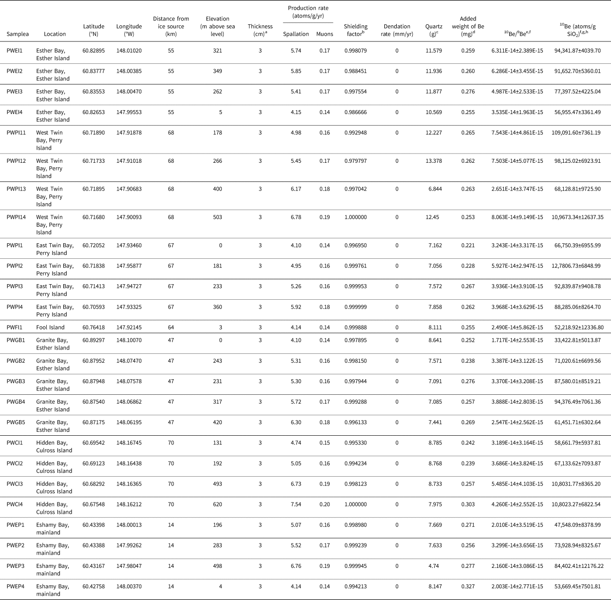
a The tops of all samples were exposed at the surface.
b Calculated using CRONUS-Earth online calculator v. 2, revised April 2018.
c A density of 2.7 g/cm3 was used based on the granitic compostion of the surface samples.
d 10Be/9Be ratio of added Be ranges between 3.26 × 10⁻¹⁵ and 8.07 × 10⁻¹⁵.
e Isotope ratios were normalized to 10Be CEREGE in house standard with a mean value of 5.60 × 10⁻¹² and using a 10Be half-life of 1.387 × 10⁶ yr.
f Uncertainties reported at the 1σ confidence level.
g Reported values are corrected for respective procedural blanks in each batch. Blank values range between 3.26 × 10⁻¹⁵ and 8.07 × 10⁻¹⁵.
h Propagated uncertainties include error in the blank and counting statistics.
Samples were collected using a hammer and chisels, and the maximum thickness of all samples collected was 3.0 cm. Samples were prepared at the Cosmogenic Laboratory of the Hebrew University of Jerusalem following procedures slightly modified from Corbett et al. (Reference Corbett, Bierman and Rood2016) and Kohl and Nishiizumi (Reference Kohl and Nishiizumi1992). Our field estimates of quartz content determined the size of the collected samples. However, during sample preparation, we found the quartz content was lower than estimated in the field, leading to a low yield. Quartz yield for each sample ranges from 4.74 to 13.38 g (Table 2). This low yield added to the relatively high uncertainty (10%–24% with an average of 13 ± 3%) of the calculated ages. 10Be/9Be ratios were measured by the accelerator mass spectrometry facility (ASTER) at CEREGE, Aix-en-Provence, France (Table 2).
For calculation of 10Be exposure ages, we used the iceTEA online interface (Jones et al., Reference Jones, Small, Cahill, Bentley and Whitehouse2019a; ice-tea.org, accessed 28 May 2021), which uses a modified version of the CRONUScalc calculation framework of Marrero et al. (Reference Marrero, Phillips, Borchers, Lifton, Aumer and Balco2016) and global production rate calibration data sets of Borchers et al. (Reference Borchers, Marrero, Balco, Caffee, Goehring, Lifton, Nishiizumi, Phillips, Schaefer and Stone2016). Within iceTEA, we used the “LSD” scaling scheme (Lifton et al., Reference Lifton, Sato and Dunai2014), which applies a sea-level, high-latitude 10Be production rate of 4.09 atoms/g SiO2/yr and a 10Be decay constant of 4.99 × 10⁻⁷/yr. We opted to use the iceTEA calculator, rather than the more common calculator, formerly known as CRONUS-Earth, because it is the only one that can also do GIA calculations. The GIA calculator includes corrections for a changing time–altitude history, such as during sea-level low stands and submergence of samples, before isostatic adjustment. Due to overcast skies and fog while collecting some samples, we opted for a uniform geographic information systems (GIS) approach to calculating topographic shielding at each site (Table 2). We used the r.horizon tool in the GRASS set of raster tools (grass.osgeo.org, accessed 28 May 2021) for the open-source QGIS software (qgis.org, accessed 28 May 2021) to calculate the angle from horizontal to the horizon at each site.
RESULTS
Overall, 10Be concentrations range between 33,423 ± 5,014 and 127,807 ± 6849 atoms/g quartz (Table 2). Sea-level elevation samples (0–5 m asl; n = 5) yielded 10Be concentrations ranging between 33,423 ± 5014 and 66,750 ± 5956 atoms/g quartz with a mean of 52,603 ± 12,127 atoms/g quartz. Apart from sample PWGB1, sea-level samples exhibit a relatively small scatter in 10Be concentrations (mean = 57,399 ± 6542 atoms/g quartz), indicating similar and straightforward exposure histories. The highest-elevation samples in each transect (349–620 m asl; n = 6) yielded 10Be concentrations that range between 61,451 ± 6303 and 109,673 ± 12,637 atoms/g quartz. These concentrations correlate weakly with elevation (r 2 = 0.26), indicating that the differences in concentrations are controlled by varying exposure histories rather than simply by elevation. This trend is also expressed by the observations that the highest 10Be concentration was measured in a sample that was collected from an elevation of only 181 m (PWPI2) and that, overall, the highest 10Be concentrations (>100,000 atoms/g quartz) were derived from samples that were collected from elevations that range between 178 and 620 m asl.
Evaluation of snow shielding and GIA on ages
10Be concentrations have simple, uncorrected, ages that range between 7.5 ± 1.0 and 24.0 ± 2.4 ka (Table 3). However, 10Be concentrations and, by inference, exposure ages are influenced by several processes, such as snow shielding and GIA, which are not considered in the uncorrected ages. Let us first consider the influence of snow cover. Before about 11 ka, global temperatures were colder than today (Seguinot et al., Reference Seguinot, Rogozhina, Stroeven, Margold and Kleman2016; Praetorius et al., Reference Praetorius, Condron, Mix, Walczak, McKay and Du2020), and we infer more snow cover at our sampling sites. Present climate is remarkably varied within the PWS region, with mean annual snowfall varying from 313 to 502 cm at weather stations within 100 km of our sampling localities (Blanchet, Reference Blanchet1983). There are few quantitative data for snow cover, in contrast to precipitation. Only one location within the study area has snow cover data: Esther Island, elevation 15 m (Natural Resources Conservation Service automated SNOTEL site (https://www.wcc.nrcs.usda.gov/snow/, accessed 28 May 2021)), has almost complete data from the interval of 2013 to 2020 and some data from three previous years. The data show snow cover from November to May, which yielded average values of November, 4.6 cm; December, 10.8 cm; January, 17.3 cm; February, 49.5 cm; March, 56.8 cm; April, 59.0; and May, 0.6 cm; a year-round average of 16.5 cm. Snow cover is also elevation dependent, as the snowpack melts more slowly at higher elevations. None of the sites have perennial snow fields today. Finally, snow cover is dependent on wind, which can be high on ridges or mountaintops, where most of our samples were collected, and can reduce or eliminate snow cover.
Table 3. Exposure ages of Prince William Sound samples.
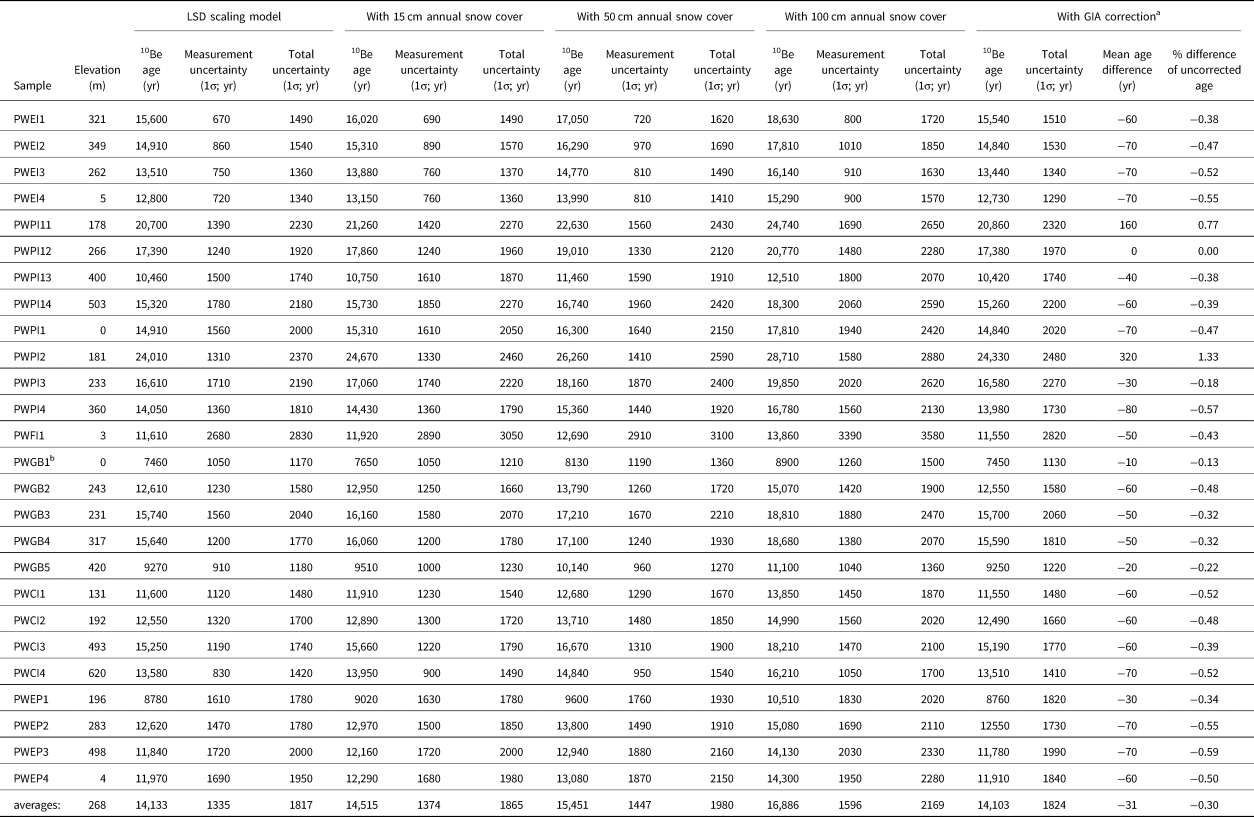
a Without a snow cover correction. GIA, glacial-isostatic adjustment.
b Culled: see text; averages at bottom of columns do not include this sample.
To evaluate the effects of snow cover, we ran several scenarios, including 15, 50, and 100 cm of annual snow cover (Table 3). As an example, if there were 15 cm of snow cover evenly on all sites for 12 months a year (a rounded average of the SNOTEL site on Esther Island), ages would average about 400 yr or 2.7% older (see Table 3). This is probably a minimum snow cover correction, but if it annually averaged 50 or 100 cm, such as at higher altitudes, and particularly before 11 ka (Seguinot et al., Reference Seguinot, Rogozhina, Stroeven, Margold and Kleman2016; Praetorius et al., Reference Praetorius, Condron, Mix, Walczak, McKay and Du2020), the correction is exponentially greater—about 1300 yr (9.3%) and 2700 yr (19.5%), respectively (Table 3). Given the lack of a reasonable way to estimate snow cover and the additional variabilities related to elevation and aspect, we did not apply a snow-shielding correction. Thus, our exposure ages are a minimum, the true ages are likely 400+ yr older, with possibly higher values at higher elevations.
10Be ages are sensitive to atmospheric depth; therefore, changes in elevation due to isostatic rebound as well as the sea-level history have the potential to affect cosmogenic radionuclide ages (Jones et al., Reference Jones, Whitehouse, Bentley, Small and Dalton2019b). In particular, it is possible that samples collected close to present-day sea level were submerged, and thus shielded, for a period of time soon after deglaciation, before isostatic rebound, and then re-exposed after GIA. Chapman et al. (Reference Chapman, Haeussler, Pavlis, Haeussler and Galloway2009) evaluated the isostatic rebound and sea-level rise at Wingham Island, Alaska (Fig. 1)—about 110 km to the southeast of PWS—in a region that likely has a similar glacial history and crustal thickness and rigidity. They assumed the total sea-level rise in southern Alaska since 20 ka was 120–135 m, and they modeled total isostatic rebound during the past 16 ka to be about 130 m. The similarity between the magnitude of sea-level rise and isostatic rebound calculated by Chapman et al. (Reference Chapman, Haeussler, Pavlis, Haeussler and Galloway2009) suggests that our samples would have remained above sea level and were not shielded by seawater. However, Chapman et al. (Reference Chapman, Haeussler, Pavlis, Haeussler and Galloway2009) argue that sea-level rise outpaced isostatic rebound between 20 and 9 ka, based on work by Clague and James (Reference Clague and James2002), who studied the British Columbia, Canada, margin. Thus, five of our samples that are located within a few meters of sea level may have been covered and shielded by seawater for part of that time period, indicating that these samples would yield minimum ages.
To calculate the effects of GIA and possible seawater shielding during sea-level rise on the 10Be ages in our study, we utilized the iceTEA set of tools (Jones et al., Reference Jones, Small, Cahill, Bentley and Whitehouse2019a). For the GIA correction, we used the ICE-6G model of Peltier et al. (Reference Peltier, Argus and Drummond2015), as it is the most advanced global model available. ICE-6G uses the deglaciation isochrones for North America from a compilation by Dyke et al. (Reference Dyke, Moore and Robertson2003). That data set is significantly more robust for deglaciation of the Laurentide and Innuitian Ice Sheets than for the CIS in Alaska. However, the general pattern and timing of deglaciation in Alaska appears to be in accord with the maximum Wisconsinan glacial extents reported by Kaufman and Manley (Reference Kaufman, Manley, Ehlers and Gibbard2004) and Kaufman et al. (Reference Kaufman, Young, Briner, Manley, Ehlers, Gibbard and Hughes2011), as well as the other constraints reported in the introduction. ICE-6G also models a global sea-level curve. The model does not account for the specific rheology for the lithosphere of southern Alaska, nor does it include more recent constraints on the mantle viscosity in southeastern Alaska (Larsen et al., Reference Larsen, Motyka, Freymueller, Echelmeyer and Ivins2005). Moreover, there are no constraints on the magnitude or timing of the GIA in PWS (Shugar et al., Reference Shugar, Walker, Lian, Eamer, Neudorf, McLaren and Fedje2014). We acknowledge these model limitations, as we lack a more robust method for evaluating GIA and sea-level rise. A unique feature of iceTEA calculations is that they will have a production rate of zero if the sample is submerged and falls below sea level.
The modeling of our results shows the iceTEA GIA correction has a small effect on the calculated ages, resulting in changes from −70 yr to +320 yr (Table 3). The average change is −31 yr, and the largest changes are with the oldest samples, which would have experienced the largest adjustment in altitude relative to sea level. All of the corrected ages are within 1.33% of the original ages. We use these elevation-corrected ages for the remainder of our discussion (Fig. 3, Table 3).
DISCUSSION AND INTERPRETATION
In spite of the uncertainties associated with our exposure ages, we proceed with our discussion assuming these calculated ages approximate the timing of bedrock exposure from deglaciation. We first discuss samples at sea level, then examine details of the variation in ages in each vertical transect, and then discuss aspects of all transects when considered together.
Sea-level samples
Exposure ages of sea-level samples can reflect a complex history, because they are most likely to be affected by GIA and sea-level rise. Five samples were collected between 0 and 5 m asl (PWEI4, PWPI1, PWFI1, PWGB1, PWEP4) and yielded exposure ages based on their present elevations that range between 7.4 ± 1.1 and 14.8 ± 2.0 ka (Fig. 3, Table 3). Given the relative proximity of the samples to one another, we would expect them to have the same GIA and sea-level history. Sample PWGB1 from Granite Bay is the youngest of our samples, and the 1σ error from this sample does not overlap the 1σ errors from any of the other samples. A kernel density estimate of the probability distribution function (Lowell, Reference Lowell1995) as implemented in iceTEA (Jones et al., Reference Jones, Small, Cahill, Bentley and Whitehouse2019a) shows the probability distribution function of this sample has some overlap with the others (Fig. 6), but because the age of this sample is significantly younger than the others, it is an outlier and does not share the same geologic history as the other samples.
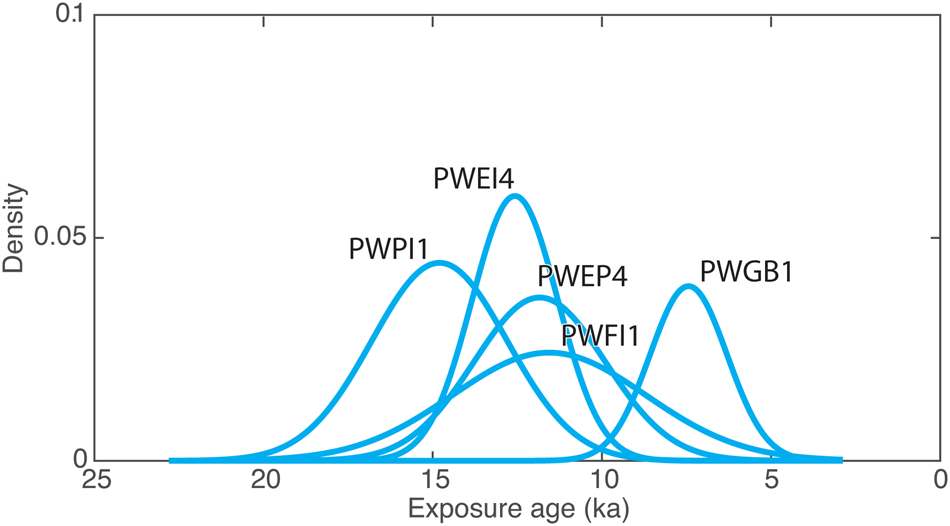
Figure 6. Kernel density distributions of 10Be exposure ages of samples collected between 0 and 5 m above sea level (m asl). Ages are glacial-isostatic adjustment corrected and use the LSD scaling model (Table 3).
There is no geologic evidence that the timing of deglaciation at sea level between the Granite Bay site and the other nearby sites should be different. The geomorphology shows no evidence of glacial stagnation between Granite Bay and the nearby bays. Alternatively, if the young age of PWGB1 is related to a glacier remaining in its valley for a longer period of time, we would expect all of the 10Be ages from this locality to be significantly younger. However, this is not the case, and the nearby Esther Bay samples have similar ages. The older postglacial radiocarbon age to the north (Table 1, Golden sample,) is also not consistent with a young sea-level age at Granite Bay. Anomalously high snow cover could shield the site and make it appear younger. However, there is no reason to hypothesize why this site, but not others nearby, would have additional snow. On reexamination of the site (Fig. 7), we determined that the smooth surface we sampled was likely caused by removal of an exfoliation slab and not by glacial scour. Parallel joint surfaces above and below the sampled surface and a few granitic boulders remain on the outcrop, consistent with debris related to breakup of an exfoliation slab. Exfoliation after glaciation is a common phenomenon (e.g., Gilbert, Reference Gilbert1904), and we infer that the smooth surface we sampled was exposed by the removal of an exfoliation slab and not by glacial scour. This would result in a lower 10Be concentration and hence a younger exposure age that does not represent the time of deglaciation. Thus, we culled sample PWGB1 from our data set. Without sample PWGB1, we infer glaciers retreated from the sea-level sites by about 12.9 ± 1.1 ka.

Figure 7. Photograph of site PWGB1 that has fractures, parallel to and above and below the surface that is being sampled, which dip to the right. We interpret these as exfoliation fractures. Photograph by PJH, U.S. Geological Survey.
Vertical transects and thinning
We plotted the GIA-corrected ages versus elevation to assess the thinning of glaciers at each site and to examine the variability of ages within and between sites (Fig. 8). Most ages lie between 9 and 15 ka (Table 3). If the data and sites provided simple records of glacier thinning, then we would expect older ages at the top and younger ages at lower elevations as glacial ice thinned (Fig. 9A). The Culross transect data form this pattern, except for the uppermost age, which is slightly younger than the next highest age, although the age lies within the error (Fig. 8C).
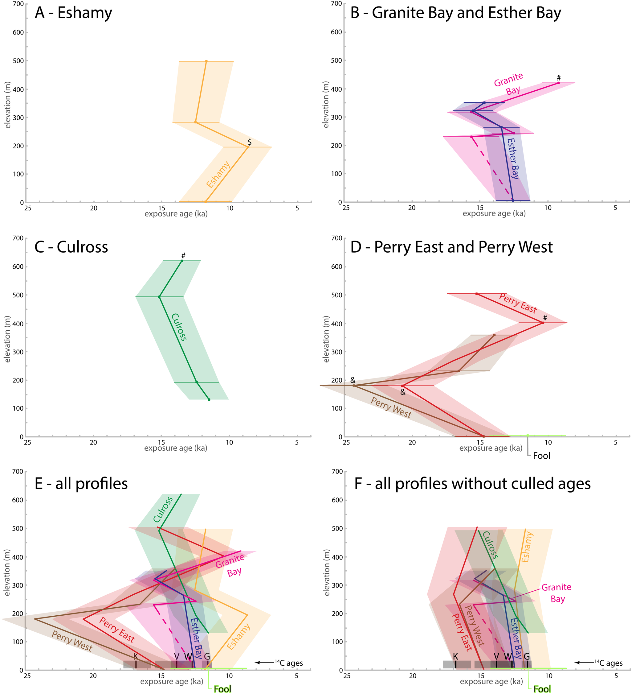
Figure 8. 10Be age–elevation plots for vertical transects in the study. Dots show sample data, with horizontal thin lines showing 1σ errors; thicker lines are drawn through calculated ages; and shaded area encompasses the 1σ errors. Vertical and horizontal scales are the same for all plots. Symbols adjacent to some samples indicate suspicions of issues with ages due to #, lingering ice, snow fields, or perennial snow cover; $, lingering cirque glacier; &, possible inheritance. See text for discussion. (A) Eshamy transect (yellow). (B) Granite Bay on Esther Island (violet) and Esther Bay (blue) plots. We plot these two together, because they are located close together on different parts of the same island (Fig. 2B). For a sea-level age for Granite Bay, we plot the sea-level age from Esther Bay. (C) Culross transect (green). (D) Perry-West (brown) and Perry-East (red) transects. We plot these together, because they lie within 2 km of each other and share the sea-level sample PWPI1. We also plot the one Fool Island sample here, as it is located about 2.5 km north of Perry Island. (E) All age–elevation transects plotted together, with the same colors as in A–D. Also shown at bottom with the black lines and gray boxes for errors are postglacial 14C ages discussed in the text: V, Valdez sample (Table 1); G, Golden sample (Table 1); K, Katalla sample (calibrated from Sirkin and Tuthill, Reference Sirkin and Tuthill1987); W, Wingham sample (calibrated from Chapman et al., Reference Chapman, Haeussler, Pavlis, Haeussler and Galloway2009). Sample locations shown on Figs. 1 or 2. (F) Plot, similar to E, except with a highly culled version of the data, in which samples PWPI2 and PWPI11 are removed for suspicion of being too old due to inheritance (denoted by & next to samples); samples PWCI1 and PWGB5 are removed for suspicion of being too young due to lingering ice, snow fields, or perennial snow cover (denoted by # next to sample); and PWEP1 (denoted by $ next to symbol) is removed for suspicion of a lingering cirque glacier.
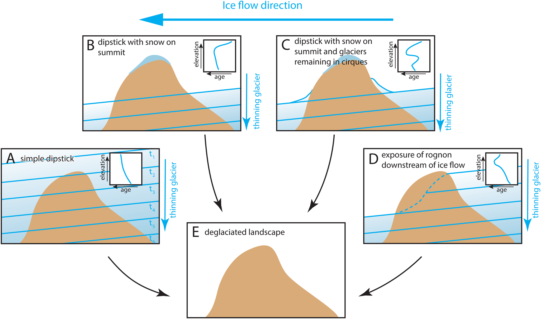
Figure 9. Cartoons showing different ways that islands can act as dipsticks in glacial flow and record thinning in surface exposure ages. View is a cross section of an island perpendicular to ice flow direction. Blue subhorizontal lines are isochrones of ice thinning at arbitrary times. Inset box shows a hypothetical age–elevation plot with the blue line showing the trend through the data. (A) Island acts as simple dipstick in ice flow, with ice thinning evenly around island. Arbitrary times t 1 (older) to t 6 (younger) are labeled here, but not in other parts of figure. (B) Simple thinning but with snow field remaining on or near summit. (C) Thinning with snow remaining on summit and with cirque glaciers feeding into the trunk glacier or alternatively remaining behind after a trunk glacier retreats. (D) Thinning of glacier exposing a rognon. (E) Final deglaciated landscape.
None of the remaining sites have similarly simple age–elevation patterns, so we considered possibilities for variations from the simple dipstick model (Fig. 9). If snow or ice remained on top of a mountain for a period of time after a glacier thinned around it—either from lingering snow and ice or due to seasonal snow cover—this would lead to younger surface exposure ages due to shielding (Fig. 9B). The only transect with significantly younger ages at the top is the Granite Bay transect, where the highest sample (PWGB5) age is 9.3 ± 1.2 ka compared with the next highest sample (PWGB4), which has an age of 15.6 ± 1.8 ka (Fig. 8B). The slightly younger age of the sample at the summit of Culross Island (PWCI4, 13.5 ± 1.4 ka) compared with the next highest sample (PWCI3), which has an age of 15.2 ± 1.8 ka, can also be explained by this mechanism, although the ages of the two samples are the same within error (Fig. 8C). The second-highest sample on the Perry East transect (PWPI13, 10.4 ± 1.7 ka; Fig. 8D) might also be explained by this mechanism. However, because the summit sample is about 5 ka older (15.3 ± 2.2 ka), it suggests a small glacier or ice field remained near the ridge where PWPI13 lies (Fig. 3C) but did not cover the summit.
Cirque glaciers and snow fields remain on the landscape longer than trunk glaciers, which explains some variations in exposure ages (Fig. 9C). The age of PWEP1 (8.8 ± 1.8 ka) from the Eshamy transect appears to fit this explanation (Fig. 8A). This sample was from the north side of a saddle, where a lingering glacier or snow field would be expected to remain after ice retreated from surrounding lower elevations. Also, the age of PWGB2 (12.6 ± 1.6 ka) from the Granite Bay transect is about 3 ka younger than nearby sample PWGB3 and next higher sample PWGB4. Both of those samples were taken from a broad ridge crest, but PWGB2 was taken at the head of a north-facing cirque. However, the age is not anomalous when compared with others in the data set (such as PWEI4, PWCI2, PWEP2). Both the Culross and Perry East transects also have samples from within cirques but do not fit this expected pattern.
Yet another scenario involves deglaciation of a rognon (an isolated rounded rock surrounded by a glacier), where rock is first exposed on the downstream side of an ice flow (Fig. 9D). None of our transects are on the downstream side of the ice flow directions, so we cannot test this. The two Perry Island ages from about 180 m elevation are the oldest in the entire data set (PWPI2, 24.3 ± 2.5 ka; PWPI11, 20.9 ± 2.3 ka; Fig. 8D.). However, they are on the upstream side of ice flow and at relatively low elevation, and the rognon mechanism cannot explain their unexpectedly old ages. We suspect some inheritance may explain their old ages, but without adjacent boulder sample ages, we cannot test this hypothesis. Inheritance occurs when ice does not erode ~2–3 m of a previously exposed rock surface. Ages can be inheritance skewed if less than that amount of rock is eroded. Inheritance has been noted in other studies (e.g., Brook et al., Reference Brook, Kurz, Ackert, Denton, Brown, Raisbeck and Yiou1993; Briner and Swanson, Reference Briner and Swanson1998), as well as in midslope settings in other Arctic regions (Young et al., Reference Young, Lamp, Koffman, Briner, Schaefer, Gjermundsen and Linge2018). Because highly erosive wet-based glaciers are expected for the PWS region, we would expect deep erosion during the LGM glaciation. Nonetheless, these unexpectedly old ages are puzzling; they point to inheritance or inheritance-skewed ages, and this mechanism might affect other samples too.
When we compare exposure histories of the vertical transects (Fig. 8E), most profiles have a crudely Z-shaped appearance, with younger ages at the high and low elevations, and the oldest ages somewhere in the middle. Where an island has more than one profile, the transects are similar. For example, on Perry Island, the vertical transects are about 2 km apart on either side of East Twin Bay (Fig. 3C) and have ages within error of each other (Fig. 8D). These profiles have the oldest exposure ages around 180 m elevation of 20.9 ± 2.3 and 24.3 ± 2.5 ka, which we suspect are influenced by inheritance, as discussed earlier. The Esther Island transects at Esther Bay and Granite Bay are about 6 km apart on different aspects of the island and have similar patterns (Fig. 8B), with maximum exposure ages at about 320 m of 15.5 and 15.6 ka. When we compare all transect age–elevation plots together (Fig. 8E), the transects vary considerably, with ages converging toward the sea-level ages between 11.6 and 14.8 ka. The vertical transect patterns thus reveal details of the deglaciation processes.
Given these possible explanations for variability in transect ages, we evaluate the potential for a quantitative record of ice thinning in our data set. As mentioned before, the Culross transect appears to be the best-behaved set of data. If we cull additional outlier ages from the other transects, based on the foregoing discussion, the age patterns are clearer (Fig. 8F). For this plot, we cull PWPI2 and PWPI11 for suspicions of their being too old due to inheritance; PWEP1 for possibly being too young due to a lingering cirque glacier; and PWCI1, PWPI3, and PWGB5 due to snow shielding, as discussed previously. In this version of the plot, the remaining 20 samples yield ages that range between 11.6 ± 2.8 and 17.4 ± 2.0 ka.
We used a calculator within iceTEA to estimate the rate of ice thinning. We assume thinning was continuous over the time period of the analysis. IceTEA uses a weighted least-squares linear regression applied randomly to a 2σ normal distribution of exposure ages through 5000 iterations of a Monte Carlo simulation (Jones et al., Reference Jones, Small, Cahill, Bentley and Whitehouse2019a). We grouped two pairs of transects to provide a more robust estimate of thinning. Because the Granite Bay and Esther Island transects are nearby and have similar values, we combined them and included the Fool Island sample as an additional sea-level age. Also, the Perry East and West transects are close to each other, and the age–elevation profiles are similar, so we combined them. We show results and statistics for the resulting four vertical transects (Fig. 10). The modal and median values, respectively, are 150 and 160 m/ka for the Culross transect (Fig. 10A), 50 and 130 m/ka for the Eshamy transect (Fig. 10B), 120 and 130 m/ka for the combined Granite Bay and Esther Bay transects (Fig. 10C), and 150 and 230 m/ka for the combined Perry East and West transects (Fig. 10D). The thinning-rate values of 120 to 150 m/ka are relatively consistent among all the transects. Although the rates encompassed by the 68% or 95% uncertainties are significantly larger, the relative consistency of the median and mode suggests they reflect the thinning process. Moreover, these regressions have a sea-level intercept consistent with the sea-level average age of 12.9 ± 1.1 ka. These thinning rates are not as high as has been documented in the northeastern United States or in Antarctica (Johnson et al., Reference Johnson, Bentley, Smith, Finkel, Rood, Gohl, Balco, Larter and Schaefer2014; Corbett et al., Reference Corbett, Bierman, Wright, Shakun, Davis, Goehring, Halsted, Koester, Caffee and Zimmerman2019), where rates are up to 590 m/ka. This difference may be due to the high topography, large catchment, and high precipitation in southern Alaska. We conclude the localities we sampled were not ideal glacial dipsticks, owing to local topography, seasonal snow cover, lingering ice, and possible cosmogenic inheritance. Nevertheless, our data reveal details of the deglaciation and erosional processes.

Figure 10. Plots of exposure age versus elevation for transects used for thinning-rate calculations. These plots use the highly culled data set described in the text. A weighted least-squares regression was applied randomly to normally distributed exposure ages (red dots and 1σ error bars) through 5000 iterations of Monte Carlo simulations (gray lines) with a positive slope using the iceTEA tool of Jones et al. (Reference Jones, Small, Cahill, Bentley and Whitehouse2019a). The statistics for these simulations are summarized in the box at the lower left of each plot, the 95% confidence limits of the thinning rate are shown with dotted black lines. (A) Culross transect, (B) Eshamy transect, (C) combined Granite Bay and Esther Bay transects, (D) combined Perry-East and Perry-West transects.
Ice retreat
We examined the data for evidence of glacial retreat. If we use the culled data set discussed in the previous section, the transect ages and distance to the paleo–ice source moderately correlate (Fig. 8F). The Eshamy transect is closest to the paleo–ice source and has the youngest ages. The Granite Bay and Esther Bay transects are similar and are next farthest from the paleo–ice source. The Fool Island sea-level sample is located 5 km from the mouth of Esther Bay, and its age (PWFI1, 11.6 ± 2.8 ka) is within error of the sea-level sample from nearby Esther Bay (PWEI4, 12.7 ± 1.3 ka). The similar Perry East and West transects have the oldest ages of any transect and are the farthest from a paleo–ice source. Moreover, the sea-level sample shared by both transects is the oldest of the sea-level population (PWPI1, 14.8 ± 2.0 ka). That this sample age is older than the nearby Fool Island and Esther Bay samples suggests the retreating ice front may have paused between Perry and Fool Islands. The two lowest ages on the Culross transect (PWCI1, 11.6 ± 1.5 ka; PWCI2, 12.5 ± 1.7 ka), when compared with the others, indicate that glacial ice lingered in this valley longer than in nearby Perry, Fool, and Esther Islands. The Culross Island samples are from Hidden Bay (Fig. 3D). The entrance to this bay is shallow (≤8 m), and the glacier filling this valley would not have been marine terminating at a sea-level low stand. Thus, during the thinning process, we infer a glacier remained in this valley longer than the adjacent marine-terminating trunk glacier.
A more analytical approach to examining retreat is by linear regression of the age and distance from ice source data. We applied the iceTEA calculator to the culled data set discussed earlier using the same method as for ice thinning. The calculated retreat rate is 20 m/yr (Fig. 11). The plot shows the regression is strongly influenced by the Eshamy data, which lie considerably closer to the ice source, and moreover, a different ice source than the other sites. Without the Eshamy transect, the ages of the remaining sites are considerably scattered and do not exhibit any clear age-versus-distance trend. Given the relatively small variation in distance to the ice source, perhaps this outcome is expected. If we assume all these ages (except Eshamy) are from one population, the weighted mean age is 14.3 ± 1.6 ka. These ages may not all be from one population due to factors already described (different elevations, snow shielding, and inheritance), but given the relative consistency of the ages and the consistent rates of thinning, we infer this is the time these mountainous islands were first exposed in this part of PWS. If we assume the Eshamy ages are from a separate population, the weighted mean of those ages is 12.2 ± 0.4 ka, indicating the Eshamy surface exposure ages are younger than the remainder of our data set. The previously discussed weighted mean of the sea-level ages is 12.9 ± 1.1 ka, which we infer is the retreat of marine-terminating glaciers past the sampling sites. The Eshamy transect ages are within the error of the sea-level ages, which indicates rapid collapse of that part of the Sargent Ice Field ice sheet.
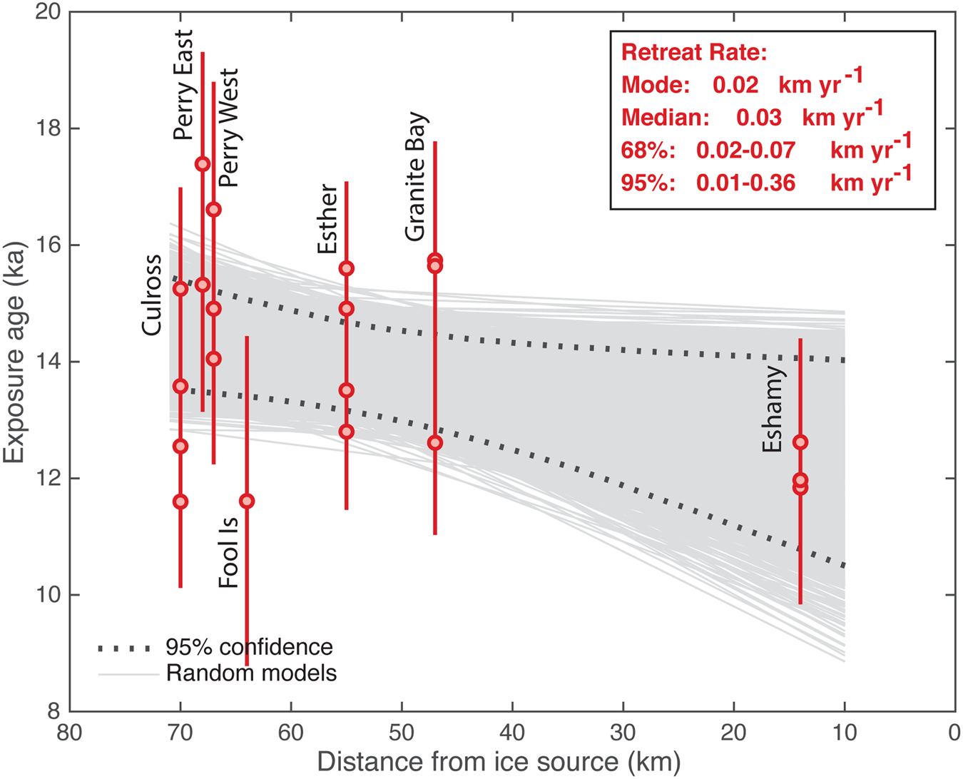
Figure 11. Exposure ages vs. distance from ice source. Transect names are labeled. The weighted least-squares regression is applied randomly to normally distributed exposure ages (red dots and 1σ error bars) through 5000 iterations of Monte Carlo simulations (gray lines) with a positive slope using the iceTEA tool of Jones et al. (Reference Jones, Small, Cahill, Bentley and Whitehouse2019a).
The retreat rate may have changed as deglaciation progressed. We assume that glaciers extended locally to the edge of the continental shelf 23 ka in cross-shelf troughs (Kaufman et al., Reference Kaufman, Young, Briner, Manley, Ehlers, Gibbard and Hughes2011; Figs. 1 and 2). The distance from Culross Island or Perry Island to the edge of the shelf is about 200 km. If we use the age of 14.3 ± 1.6 ka for removal of ice near Perry, Culross, and Esther Islands, then ice would have retreated 200 km between 23 and 14.3 ka, or during an interval of 8.7 ka. This yields a retreat rate of 23 m/yr, which is about the same rate (20 m/yr) that we calculated between our sites closer to the source of the ice. If retreat from the shelf edge was later, at ~17 ka, as suggested by Misarti et al. (Reference Misarti, Finney, Jordan, Maschner, Addison, Shapely, Krumhardt and Beget2012) and Lesnek et al. (Reference Lesnek, Briner, Baichtal and Lyles2020), then the initial retreat rate would have been 74 m/yr, which then slowed to 20 m/yr as glaciers receded toward the higher mountains that could generate more ice.
REGIONAL COMPARISONS AND GLOBAL LINKAGES
Our PWS surface exposure ages help to clarify ice retreat patterns of the northernmost marine-terminating glaciers of the CIS (Fig. 12). The two postglacial radiocarbon ages in PWS are consistent with our surface exposure ages. The older of the two basal peat ages (14,020 ± 770 cal yr BP; Reger, Reference Reger1990; Fig. 12, Table 1) is nearly the same as the weighted mean of our 10Be ages (14.3 ± 1.6 ka, excluding the Eshamy transect), and the 14C age is slightly younger, as expected when allowing for the growth of vegetation. This older 14C age is from a site near Valdez, 95 km away on the east side of PWS. The similarity of the 14C and 10Be ages suggests that the timing of deglaciation in eastern PWS is similar to western PWS, as one might expect because of the similar physiographic setting. The younger 14C age (11,580 ± 220 cal yr BP; Heusser, Reference Heusser1983; Fig. 12, Table 1) is slightly younger than the average of our near sea-level samples (12.9 ± 1.1 ka; see also Fig. 8). The site for the younger 14C age is about 10 km north of our northernmost samples (Fig. 2), which is consistent with the model of northward-retreating glaciers.
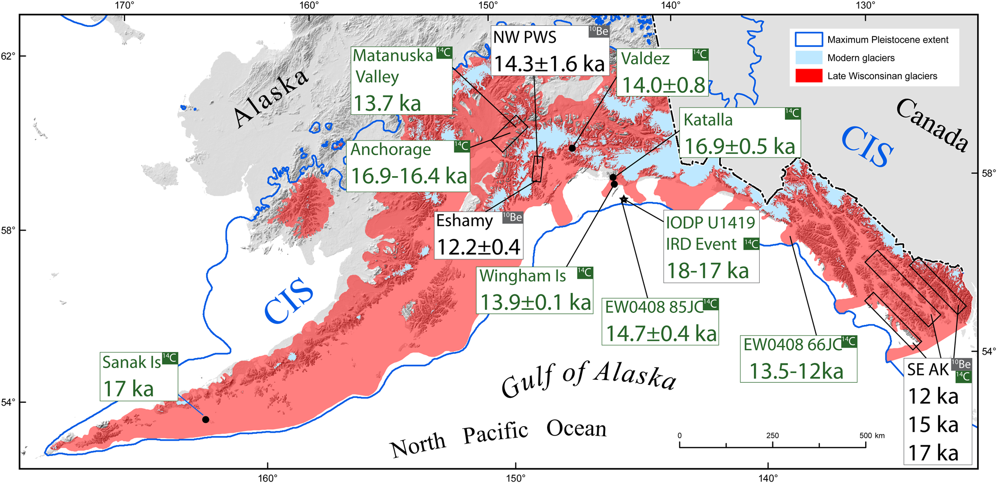
Figure 12. Map showing ages of late Quaternary deglaciation along the Alaskan margin. Boxes show deglaciation locality and ages. Ages in black are from cosmogenic surface exposure dates. Ages in green are earliest postglacial radiocarbon dates. Sources of data: Sanak Island from Misarti et al. (Reference Misarti, Finney, Jordan, Maschner, Addison, Shapely, Krumhardt and Beget2012), Anchorage and Matanuska Valley from Kopczynski et al. (Reference Kopczynski, Kelley, Lowell, Evenson and Applegate2017), Eshamy and NW Prince William Sound (PWS) from this study, Valdez from Reger (Reference Reger1990), Wingham Island from Chapman et al. (Reference Chapman, Haeussler, Pavlis, Haeussler and Galloway2009), Katalla from Sirkin and Tuthill (Reference Sirkin and Tuthill1987), southeastern Alaska (SE AK) from Lesnek et al. (Reference Lesnek, Briner, Baichtal and Lyles2020), and IODP core U1419 from Walczak et al. (Reference Walczak, Mix, Cowan, Fallon, Fifield, Alder and Du2020). Base map showing extent of late Wisconsinan (approximately last glacial maximum) and Pleistocene maximum extent of glaciers in Alaska, from Kaufman et al. (Reference Kaufman, Young, Briner, Manley, Ehlers, Gibbard and Hughes2011). Extent of Cordilleran Ice Sheet (CIS) in Canada from Batchelor et al. (Reference Batchelor, Margold, Krapp, Murton, Dalton, Gibbard, Stokes, Murton and Manica2019).
The timing of ice retreat of the CIS in PWS appears to be similar to some phases of ice retreat elsewhere along the southern Alaska margin. As mentioned earlier, Davies et al. (Reference Davies, Mix, Stoner, Addison, Jaeger, Finney and Wiest2011) interpreted core EW0408 85JC (Fig. 12) from offshore and southeast of PWS as having a transition from coarse glacial-marine sediments to finely laminated sediments at 14,790 ± 380 cal yr BP. They interpreted this date as the time that tidewater glaciers to the north retreated onto land or behind fjord sills. Their age is similar to our result. Due north of this core, at a terrestrial site in the coastal Katalla River valley (Figs. 2A and 12), Sirkin and Tuthill (Reference Sirkin and Tuthill1987) reported a postglacial radiocarbon age of 16,850 ± 550 cal yr BP (Table 1). This age implies deglaciation was locally underway along the coast east of PWS significantly earlier than in northern PWS or offshore. Chapman et al. (Reference Chapman, Haeussler, Pavlis, Haeussler and Galloway2009), in a study of Wingham Island, another coastal site 15 km east of Katalla and about 220 km to the east of our study sites (Figs. 1 and 12), obtained a 14C age of 13,890 ± 80 cal yr BP (Table 1) on a terrace, close to modern sea level, which formed after ice retreat. The Wingham Island date is similar to the weighted mean of most of our ages of 14.3 ± 1.6 ka and is older than our sea-level site ages of 12.9 ± 1.1 ka. Given the proximity of the Wingham site to the Katalla River valley (25 km apart), the difference in the radiocarbon ages is surprising, with the Katalla River valley being deglaciated approximately 3000 yr earlier than the nearby and more distal Wingham Island site.
Sanak Island, which lies about 1100 km to the southwest of PWS (Fig. 12), provides another constraint for the timing of deglaciation on the southern Alaska margin. Misarti et al. (Reference Misarti, Finney, Jordan, Maschner, Addison, Shapely, Krumhardt and Beget2012) studied lake cores and concluded that deglaciation initiated by ~17 ka, as indicated by radiocarbon and pollen data. Just north of PWS, on the leeward side of the Chugach Mountains in the Anchorage area, Kopczynski et al. (Reference Kopczynski, Kelley, Lowell, Evenson and Applegate2017) found that initial retreat of glaciers (Figs. 1 and 12) occurred between 16.8 and 16.4 ka, and a second faster phase of retreat was completed by 13.7 ka. The older time period is very similar to the Sanak and Katalla ages, and the younger age is similar to both the Wingham Island age and our ages, which suggests that retreat of glaciers in the Anchorage area before 13.7 ka (Kopczynski et al., Reference Kopczynski, Kelley, Lowell, Evenson and Applegate2017) was almost synchronous with the main pulse of thinning in northern PWS. The Perry Island ages of 16.6 ± 2.3 and 17.4 ± 2.0 ka at our most oceanward site are similar to the older ages in the Anchorage area, suggesting that warming was concurrent on both sides of the Chugach Mountains, although the northern, drier side of the Chugach Mountains was deglaciated before the southern, wetter side of the mountains of northern PWS. This inference is consistent with the recent results of Valentino et al. (Reference Valentino, Owen, Spotila, Cesta and Caffee2021), who used cosmogenic isotopes to date deglaciation of higher-elevation sites (568–1678 m) within the Chugach Mountains near Anchorage and Valdez and obtained ages between ~26.7 ± 2.4 and 17.3 ±1.5 ka.
Southeastern Alaska ages of deglaciation show similar patterns. About 700 km southeast of PWS, Praetorius and Mix (Reference Praetorius and Mix2014) studied core EW0408 66JC offshore Cross Sound and inferred significant landward retreat of glaciers between ~13 and 12.5 ka based on changes in sediment type and radiocarbon dating (Fig. 12). This time period is similar to our sea-level ages. About 1000 km to the southeast of PWS, in the fjords of southern southeastern Alaska, Lesnek et al. (Reference Lesnek, Briner, Baichtal and Lyles2020) found the most rapid phase of glacial retreat on the outer coast took place between ~17 and 15 ka, and most inner fjords were free of ice by 15 ka (Fig. 12). Their work utilized 40 10Be exposure ages and 25 radiocarbon ages and is currently the most robust terrestrial data set constraining deglaciation of the northern marine-terminating part of the CIS. The 17 ka age is the same as the Sanak Island age as well as the oldest phase of deglaciation in the Anchorage region. Despite the larger uncertainties in our data set, the younger southeast Alaska 10Be ages appear to precede those of PWS by 1–2 ka. Because the oceanographic, storm trajectory, and bathymetric conditions of southeastern Alaska and PWS are similar, the higher latitude and higher mountains of northern PWS may be the cause of the difference in ages between the two regions.
The timing of ice retreat in PWS and other marine-terminating parts of the CIS was preceded by warming sea-surface temperatures. Praetorius et al. (Reference Praetorius, Condron, Mix, Walczak, McKay and Du2020) compiled records of northeastern Pacific sea-surface temperature data that show warming from 17 ka into the Bølling event, which started at 14.6 ka. The data show slight cooling through the Younger Dryas period, followed by warming at about 12.1 ka. These time periods and temperature transitions are reflected in the deglacial history in the North Pacific, with the oldest pulses of deglaciation around 17 ka in southern southeast Alaska, Katalla, the Anchorage region, and Sanak Island. Widespread, and perhaps catastrophic deglaciation occurred during the Bølling period in northern PWS, offshore in core EW0408 85JC, Wingham Island, Valdez, and slightly later in the Anchorage area (Fig. 12).
Our study contributes to a growing body of evidence that collapse of the CIS was an important precursor to global climate change events. As discussed earlier, the initial retreat of CIS marine-terminating glaciers was likely caused by ocean warming (Praetorius et al., Reference Praetorius, Mix, Walczak, Wolhowe, Addison and Prahl2015, Reference Praetorius, Condron, Mix, Walczak, McKay and Du2020) and dramatic sea-level rise (Spratt and Lisiecki, Reference Spratt and Lisiecki2016), with the later stages of deglaciation possibly driven by atmospheric warming (e.g., Shakun et al., Reference Shakun, Clark, He, Marcott, Mix, Liu, Otto-Bliesner, Schmittner and Bard2012). Walczak et al. (Reference Walczak, Mix, Cowan, Fallon, Fifield, Alder and Du2020) recently dated the presence of North Pacific ice-rafted debris (IRD) events at IODP Site U1419, about 200 km to the southeast of PWS (Fig. 12). The IRD events (termed “Siku events”) are thought to indicate major ice sheet retreat. The events were constrained by 250 14C dates and are similar to the Heinrich events of the North Atlantic but predate them by 1370 ± 550 yr. The youngest of these IRD events was between 18,000 and 17,000 yr BP. This time is consistent with, and slightly older than, terrestrial postglacial ages from Sanak Island, the Anchorage area, the Katalla River valley, SE Alaska, and this study (Fig. 12). Thus, this study adds to the evidence that the collapse of the CIS was early in a sequence of global climate change events, postdating strong Asian monsoons and predating North Atlantic Heinrich events, Antarctic warming, and global CO2 rise (Walczak et al., Reference Walczak, Mix, Cowan, Fallon, Fifield, Alder and Du2020).
Finally, our observations suggest a two-stage model for the development of the fjordland topography in PWS during glacial retreat. In the first stage at glacial maxima, ice flowed from the highest topography toward the middle of PWS, over lower topography, such as over the top of Perry Island (Fig. 5C). The bathymetry of the sound (Fig. 2) shows that ice flowed out via Hinchinbrook Entrance and Montague Strait, and it reached the edge of the continental shelf along cross-shelf troughs (e.g., Kaufman and Manley, Reference Kaufman, Manley, Ehlers and Gibbard2004; Kaufmann et al., Reference Kaufman, Young, Briner, Manley, Ehlers, Gibbard and Hughes2011). In the second stage, as marine-terminating trunk glaciers thinned and retreated, the glacial flow direction sometimes changed drastically. For example, the CFPW glacier (Fig. 2B) thinned, and ice flow oriented itself downhill of newly exposed mountainside slopes, perpendicular to the earlier flow direction (Fig. 4). The change in direction of ice flow from times of glacial maxima to a different direction after the retreat of tidewater glaciers explains the common large fjords and glacial valleys, which are cut at a high angle by younger and smaller glaciers in PWS topography.
The Quaternary history of this region is ripe for further study. With respect to improving the 10Be record of deglaciation, a larger sample volume, boulder–bedrock pairs, and a denser sampling scheme would improve results and decrease errors. Granitic bedrock seems to be the most viable rock type for CRN dating, and additional granites in north-central and eastern PWS would make good targets. In addition, quantitative data are needed to constrain GIA (e.g., Shugar et al., Reference Shugar, Walker, Lian, Eamer, Neudorf, McLaren and Fedje2014), and how GIA is modulated by a subduction megathrust directly below sites loaded with ice should be evaluated. Coring and high-precision 14C dating in glacial troughs both offshore and within PWS are needed to gain data on the timing and conditions of deglaciation and to better evaluate the drivers of deglaciation.
CONCLUSIONS
This is the first 10Be study of deglaciation in the PWS region of Alaska. We obtained 26 10Be surface-exposure ages from glacially scoured bedrock surfaces (Figs. 3 and 4). The samples were collected from six localities that span elevation transects where summits were rounded and overrun by LGM glaciers between sea level and 620 m. Ages range between 24.3 ± 2.5 and 8.8 ± 1.8 ka and average 14.0 ± 1.8 ka (Table 3). We evaluated the effects of snow cover on the ages and estimate shielding from snow cover would push the ages older by at least 400 yr. To assess the effects of GIA and sea-level rise and potential shielding on the exposure ages, we utilized the iceTEA set of tools (Jones et al., Reference Jones, Small, Cahill, Bentley and Whitehouse2019a) and found these processes did not have a significant effect. Samples collected near sea level have ages consistent with being from a population that averages to 12.9 ± 1.1 ka.
We evaluated simple and more complex models of ice thinning and retreat. Of the six elevation transects, we found that only the Culross Island transect ages can be readily explained by a simple model of ice removal with oldest ages at the top and younger ages down low (Fig. 8). We evaluated deglaciation processes that would affect other age–elevation profiles (Fig. 9) and infer some sample ages were influenced by lingering snow and ice and possible cosmogenic inheritance. We were unable to directly test for 10Be inheritance, because we were unable to find paired boulder and bedrock surfaces to sample. We culled additional ages that may have been affected by lingering ice and inheritance, and the remaining ages were between 17.4 ± 2.0 and 11.6 ± 2.8 ka.
We assessed rates of thinning and ice retreat from our sample transects. We calculated ice-thinning rates using a Monte Carlo approach implemented in the iceTEA calculator. We grouped data into four vertical transects and found thinning rates are between 120 and 160 m/ka based on the median and mode of the probability distributions (Fig. 10). We also found evidence of a correlation between the ages of each transect and the distance to the paleo–ice source. Considering all the sites and using the same Monte Carlo approach implemented in iceTEA, we calculated a retreat rate of 20 m/yr (Fig. 11). The Eshamy transect is unique among our sample transects, in that it is located closer to its paleo–ice source, the Sargent Icefield, than the other more northerly transects, which have an ice source in the College Fiord region. The Eshamy transect has a younger set of ages, which give a weighted mean of 12.2 ± 0.4 ka, in contrast to the mean of the ages from the other northerly sites of 14.3 ±1.6 ka. We infer this older age indicates when ice retreated from our sample sites in the mountains, and the sea-level weighted mean age of 12.9 ± 1.1 ka is the approximate time that tidewater glaciers retreated past the low-elevation sites in northern PWS. These ages are consistent with the two limiting radiocarbon ages for deglaciation in PWS. One of these ages is from the northeast side of the sound and, given its similarity to our ages, suggests that all parts of the sound had a similar deglaciation history.
Regional comparisons of these new ages show the timing of ice retreat in PWS appears to be similar to some phases of ice retreat elsewhere along the southern Alaska margin (Fig. 12). The thinning of the glaciers in northwestern PWS is within error of the time of retreat of glaciers on the northwest side of the Chugach Mountains in the Anchorage region, on Wingham Island to the southeast of PWS, and from cores offshore the Yakutat region and southeast Alaska. However, retreat of the marine-terminating glaciers, as indicated by the Eshamy transect, appears to be later, and may have been synchronous with collapse of part of the Sargant Icefield. Nonetheless, our study adds to a growing body of evidence that collapse of the CIS soon after 17 ka was early in a sequence of global climate change events, postdating strong Asian monsoons and predating North Atlantic Heinrich events, Antarctic warming, and global CO2 rise (Walczak et al., Reference Walczak, Mix, Cowan, Fallon, Fifield, Alder and Du2020).
Acknowledgments
Thanks to Kara and Katie Haeussler for help in sample collection and to Keith Labay for help with drafting of some of the figures. Thanks to editor Derek Booth, associate editor Yeong Bae Seong, two anonymous reviewers, and John Jaeger for exceptionally constructive journal reviews; Adrian Bender, Sue Karl, Marti Miller, and Janet Slate for their reviews; and Jason Addison for additional input. Fieldwork was funded by the U.S. Geological Survey; the Hebrew University Jerusalem funded analysis of samples. Any use of trade, firm, or product names is for descriptive purposes only does not imply endorsement by the U.S. government.


 Open access