1 INTRODUCTION
Maps of the sky have been produced throughout the cultural history of mankind. They represented the patterns in the sky, long believed to be static, for navigation and time-keeping, they provided a reference for measuring motions and allowed the identification of transient objects. Over time, we came to understand our place in the Milky Way and the Universe at large, and discovered new phenomena such as novae and supernovae. From motions of celestial bodies, we inferred the form and parameters of fundamental laws in physics such as the law of gravity and derived the existence of dark matter.
In modern times, digital surveys such as the Sloan Digital Sky Survey (SDSS; York et al. Reference York2000) have revolutionised the speed and ease of making new discoveries. Instrumental limitations imply that surveys need to strike a balance between depth and areal coverage. The SDSS, e.g., imaged ~70% of the Northern hemisphere sky. In contrast, the SkyMapper Southern Survey presented here covers the entire Southern hemisphere. Many surveys carried out from space-based telescopes aim for all-sky coverage, e.g., the Gaia survey (Gaia Collaboration et al. 2016a, 2016b), the survey by the Widefield Infrared Survey Explorer (WISE; Wright et al. Reference Wright2010), the X-ray surveys from the Roentgen Satellite (ROSAT; Voges et al. Reference Voges1999) and the eROSITA mission (Merloni et al. Reference Merloni2012). These missions do not replace but complement each other by observing the sky at different wavelengths, which allows us to see different physical components of the matter in the Universe, or they have different specialities such as Gaia’s high-precision astrometry, and they observe the sky at different times thus revealing variable phenomena at different stages.
Currently, a complete multi-colour inventory of the Southern sky to a depth of g, r ≈ 22, similar to the SDSS in the Northern sky, is missing, and one aim of the SkyMapper project is to fill this gap. However, SkyMapper is not a Southern copy of the SDSS in the North, in the way in which, e.g., the 2 Micron All-Sky Survey (2MASS; Skrutskie et al. Reference Skrutskie2006) used two telescopes in two hemispheres to create a consistent all-sky dataset from the ground. The SDSS in the North was especially successful in revealing new knowledge about distant galaxies, which should appear similar in the South given we live in an approximately isotropic Universe. Instead, SkyMapper aims for new discovery space beyond just repeating the SDSS in another hemisphere:
-
1. One focus of SkyMapper is studying the stars in our Milky Way, where the hemispheres are very different from each other. The Southern sky includes the bulge and centre of our Milky Way, as well as our two largest satellite galaxies, the Magellanic Clouds. Currently, we expect that the oldest stars in the Milky Way will be found in the bulge, and SkyMapper has indeed found the oldest currently known examples there (Howes et al. Reference Howes2015).
-
2. The SkyMapper filters differ from SDSS filters mainly in splitting the SDSS u-band into two filters: while the SDSS filter has (λcen/FWHM) = (358nm/55nm), SkyMapper has a violet v-band (384/28) and a more ultraviolet u-band (349/42). This choice of filters adds direct photometric sensitivity to the surface gravity of stars via the strength of the Hydrogen Balmer break driving changes in the u − v colour, as well as to their metallicity via metal lines affecting the v − g colour. By exploiting this information, SkyMapper has found the most chemically pristine star currently known (Keller et al. Reference Keller2014). We note that the other filters, griz, differ from their SDSS cousins in central wavelength and width by up to 40 nm (see Table 1, and Figure 17 for colour terms).
-
3. Southern galaxies are of special interest when their distances are below, e.g., 500 Mpc, as the distinct large-scale structure creates environments that differ from the ones in the North. While the Northern hemisphere has the iconic Virgo and Coma galaxy clusters, as well as the CfA2 and SDSS Great Walls (Geller & Huchra Reference Geller and Huchra1989; Gott et al. Reference Gott, Jurić, Schlegel, Hoyle, Vogeley, Tegmark, Bahcall and Brinkmann2005), the South distinguishes itself with the Shapley supercluster and the Southern extension to the Virgo Cluster.
-
4. As no ground-based telescope can observe the entire sky across two hemispheres, the synergy of combining data from different telescopes is limited by their location. Several cutting-edge wide-field radio telescopes are now being built in the Southern hemisphere, including the Australian SKA Pathfinder (ASKAP; Johnston et al. Reference Johnston2007, Reference Johnston2008) and the Murchison Widefield Array (MWA; Tingay et al. Reference Tingay2013) observing low radio frequencies, as well as the future Square Kilometre Array (SKA; Carilli & Rawlings Reference Carilli and Rawlings2004). ASKAP and MWA are creating deep maps of the radio sky across more than the Southern hemisphere, and providing them with a homogeneous optical reference atlas is a major mission for SkyMapper.
-
5. More generally, cosmic dipoles have fundamental importance for understanding our place and motion within the Universe, and they may reveal new physics beyond the Standard Model. Without an all-sky view, the Cosmic Background Explorer (COBE; Lineweaver et al. Reference Lineweaver, Tenorio, Smoot, Keegstra, Banday and Lubin1996) would have had a hard time measuring the motion of our Milky Way relative to the microwave background, which is a frame of reference on a scale large enough to not be dominated by its own peculiarities. Without an all-sky dataset, Blake & Wall (Reference Blake and Wall2002) would not have corroborated this cosmic dipole by referring to distant radio galaxies. Current debates concern, e.g., a cosmic dipole in the fine-structure constant of electrodynamics (e.g., Webb et al. Reference Webb, Murphy, Flambaum, Dzuba, Barrow, Churchill, Prochaska and Wolfe2001; Murphy, Malec, & Prochaska Reference Murphy, Malec and Prochaska2016), and this work would greatly benefit from samples of quasi-stellar objects (QSOs) that cover most of the sky from pole to pole. SkyMapper will provide critical coverage of the Southern hemisphere to advance such studies.
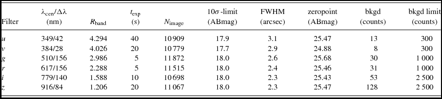
Table 1. Properties of SkyMapper DR1 imaging data. 10σ-limits are quoted for the average object in the master catalogue. The PSF FWHM, zeropoint, and background are median values among the 66 840 individual exposures. Most uvgri images are read-noise limited in the Shallow Survey. R band is a reddening coefficient from a Fitzpatrick (Reference Fitzpatrick1999) law with R V = 3.1.
In the SDSS, spectroscopy was an integral part of the project, carried out at the same facility when the seeing was better matched to the task of feeding large fibres than to taking sharp images of the sky. From the start, SDSS planned to take a million spectra of bright galaxies as well as other objects of special interest, and over time the facility has been extended to allow dedicated spectroscopic surveys for several hundreds of thousands of stars, as well as over a million luminous red galaxies (LRGs) and nearly 300 000 QSOs (Alam et al. Reference Alam2015; Blanton et al. Reference Blanton2017).
SkyMapper, in contrast, was planned from the start as a pure imaging project, with periods of poor seeing dedicated to a transient survey (Scalzo et al. Reference Scalzo2017) that finds supernovae by repeatedly imaging part of the sky, while using the main Southern Survey as a reference. Spectroscopy of a large number of objects was always going to be possible using the AAOmega spectrograph at the fibre-fed 2-degree Field facility (Sharp et al. Reference Sharp2006) at the 3.9-m Anglo-Australian Telescope, which can take spectra of nearly 400 objects simultaneously. Also, the detailed photometry of SkyMapper provides great power to preselect rare objects of interest, such as extremely metal-poor (EMP) stars, and helps to minimise the number of spectra that might otherwise be required.
However, Australian expertise in multi-fibre instrumentation has now led to a new instrument for multi-object spectroscopy that greatly reduces the cost per spectrum in massive spectroscopic surveys. The new Taipan facility currently being commissioned at the UK Schmidt Telescope is expected to take up to a million spectra of stars and galaxies per year, and the eponymous Taipan galaxy survey will use SkyMapper for its source selection (da Cunha et al. Reference da Cunha2017). One of its science goals is studying bulk flows in the local Universe from a peculiar velocity survey, and these can be much better constrained when data from both hemispheres are combined.
While all these projects have their primary science drivers, we cannot overestimate their legacy value. As the datasets become available, the community of researchers finds new answers in established data repositories by asking new, creative questions that were not part of the initial project plan. In the long run, such legacy findings dominate the scientific output of most large projects that share their data with the broad community.
In this paper, we present the first Data Release of the SkyMapper Southern Survey (SMSS DR1).Footnote 1 This first major release presents data from the Shallow Survey covering nearly the whole Southern hemisphere. The master catalogue contains ~285 million unique astrophysical objects over 20 200 deg2 of sky, while the photometry catalogue contains measurements of over 2.1 billion individual detections made in over 66 000 images. The catalogue is largely complete for objects of magnitude ~18 in all six filters across an area of 17200 deg2 and has saturation limits ranging from magnitude 8 to 9 depending on the filter and seeing. All SkyMapper magnitudes are in the AB system (Oke & Gunn Reference Oke and Gunn1983). The specific release version described in this paper is DR1.1, which is released simultaneously to Australian astronomers and the world public as of December 2017. DR1.0 was released to the Australian community in June 2017, and used a different set of calibrator stars, which led to less well-calibrated photometry. Going to DR1.1, we were also able to identify and exclude a small fraction of poorly calibrated images from the dataset.
The next release in preparation, DR2, will include images from the SkyMapper Main Survey that will reach 3–4 mag deeper, depending on the passband. Completing the Main Survey on the whole hemisphere will take until the year 2020. Even a decade from now, when data from the Large Synoptic Survey Telescope (LSST) will reach deeper into the Southern sky than any wide-field telescope before it, the SkyMapper Southern Survey will remain relevant, as it probes a different regime in brightness. All sources from this release will appear saturated and thus unmeasurable in LSST images, while the deeper SkyMapper Main Survey may assist in calibrating the LSST surveys, and adds several years to the time baseline in the study of variable phenomena with LSST. Finally, LSST lacks an equivalent to the v-band, such that SkyMapper will remain a source of important information on stellar parameters for brighter sources.
This paper is organised as follows: in Section 2, we give a short overview over the SkyMapper telescope and instrumentation, and summarise the main activities at the telescope; in Section 3, we describe the SkyMapper Southern Survey, while Section 4 details the procedures of the Science Data Pipeline (SDP), with a focus on the Shallow Survey and the resulting properties of the DR1 data; in Section 5, we discuss data quality and photometric comparisons; in Section 6, we explain data access methods as well as the database schema, and show a few example applications with database queries and results; finally, Section 7 provides an outlook to the future of the survey.
2 SKYMAPPER
SkyMapper is a purpose-built, optical wide-field survey facility located at Siding Spring Observatory near Coonabarabran in New South Wales, Australia, at the edge of the Warrumbungle National Park, which is Australia’s first declared Dark Sky Park. It has a 1.35-m primary mirror and uses a mosaic of 32 CCDs, each having 2048 × 4096 pixels with a scale of ~0.5 arcsec. The 268 million pixels cover a nearly square field-of view measuring 2.4 × 2.3 deg2. After the commissioning phase ended in March 2014, observations for the Southern Survey started. The telescope is fully robotic and nightly survey operations are planned by autonomous scheduler software that can execute the entire survey without needing human intervention.
2.1. Surveys and operations
The public SkyMapper Southern Survey claims 50% of the observing time on the SkyMapper Telescope, with a focus on good-seeing time, while bad-seeing time since 2015 has been used for the SkyMapper Transient Survey, a supernova survey described by Scalzo et al. (Reference Scalzo2017), and a fraction of time is kept available for third-party programmes. The public Southern survey contains two components with different depth and saturation limits.
The Shallow Survey targets the entire Southern hemisphere with short exposures, ensuring full-hemisphere coverage early in the project and a bright saturation limit. Several dithered visits aim at fully covering the target area despite gaps in the CCD mosaic, and repeat observations to ascertain the static or transient nature of any detected sources. During each visit, a six-colour sequence is observed within less than 5 min. While the first year of SkyMapper survey operations was dedicated mostly to the Shallow Survey, this now continues only in the brightest nights around full moon. The Shallow Survey is complete to nearly magnitude 18 in all six bands uvgriz and provides the calibration reference for the following Main Survey.
The Main Survey targets the same sky area in the same six bands, but aims to be complete to g, r ≈ 22. In combination with the Shallow Survey, the entire SkyMapper Southern Survey will provide calibrated uvgriz photometry from magnitude 9 to 22. The Main Survey includes two six-colour sequences, each taken within a 20-min interval, as well as additional visits to collect pairs of gr and iz images. The gr pairs are acquired under dark and grey sky, while the iz pairs are primarily collected in the period between astronomical and nautical twilight.
SkyMapper’s regular operations model includes daily calibration procedures including bias frames, twilight flatfields, and several visits to dedicated SkyMapper standard fields during the night. Eight such standard fields have been defined, each of which includes a Hubble Space Telescope (HST) spectrophotometric standard star. These standard field observations have not been used for DR1, but will be utilised in future releases. A paper with more complete technical and procedural references is in preparation (Onken et al. in preparation).
2.2. Filters
The SkyMapper filters are described in detail in Bessell et al. (Reference Bessell, Bloxham, Schmidt, Keller, Tisserand and Francis2011). The filters u, v, g, and z all comprise coloured glass combinations; the r-filter was made by combining magnetron-sputtered short- and long-wave passband coatings; the i-filter is coloured glass plus a short-wave passband coating; the z-band long-wavelength cut-off is defined by the cut-off in the CCD sensitivity. All filters had two-layer anti-reflection coatings applied. The diversity in fabrication methods for the SkyMapper griz filters helps explain why their passbands differ in width and placement from the SDSS griz passbands.
After polishing, the u and v bandpass glasses were slightly thinner than anticipated. As a result, they have red leaks near 700 nm, around 1% for u and much less for v. These are evident in u-band observations of K and M stars (see Figure 1).
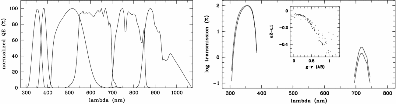
Figure 1. Normalised transmission curves for SkyMapper filters including atmosphere, telescope, and detector from Bessell et al. (Reference Bessell, Bloxham, Schmidt, Keller, Tisserand and Francis2011). Note that SkyMapper has an ultraviolet u-band and a violet v-band, where SDSS has only a single u-band. Central wavelengths and filter widths of griz-filters vary up to 40 nm relative to their SDSS cousins. Right: u-band filter curve including atmosphere, telescope, and detector, for airmass 1 and 2. The red leak at 700–750 nm wavelength increases relative to the main transmission band with airmass, because UV light is heavily absorbed by the Earth’s atmosphere, while far-red light remains nearly unaffected. As a result, the measured u-band magnitudes of red stars increase with airmass as the relative contribution from the leak increases.
The transmission curves of the filters are shown in Figure 1, they were measured at many places across the aperture and averaged to provide the mean filter passband. The all-glass filters u, v, g, and z have remarkably uniform wavelength transmission with position and with changing field angle. The interference filter defined edges on the r- and i-filters, however, change slightly with angle. The average transmission was then multiplied with one airmass of atmospheric extinction and the mean QE response curve of the E2V CCDs. The CCD response curves and the interference coatings may change over the period of the survey and thus our calculated SkyMapper passbands may need adjustment. This investigation is beyond the scope of DR1 and will be assessed from observations of our spectrophotometric standard stars.
2.3. Detector properties
SkyMapper’s 32 detectors are arranged in four rows of eight CCDs, with horizontal spaces of ~0.8 arcmin between the mosaic columns, a small gap of ~0.5 arcmin between the central rows, and larger gaps of ~3.2 arcmin separating the two upper rows from each other and the two lower rows from each other. The read-out noise of the amplifiers varies broadly between 6 counts and 14 counts. In Shallow Survey exposures, fringes are only apparent in the i- and z-band. As their amplitude is below the read-out noise, we do not defringe any of the DR1 data released here.
Figure 2 shows the efficiency curves of the 32 CCDs after normalising them at 500 nm wavelength. Variations in the blue sensitivity are already evident around 400 nm, which means that the uvg passbands will differ from CCD to CCD, with corresponding subtle differences in the zero-point (ZP) calibration and colour terms. These variations are not considered in this data release, but will be included in a future release.
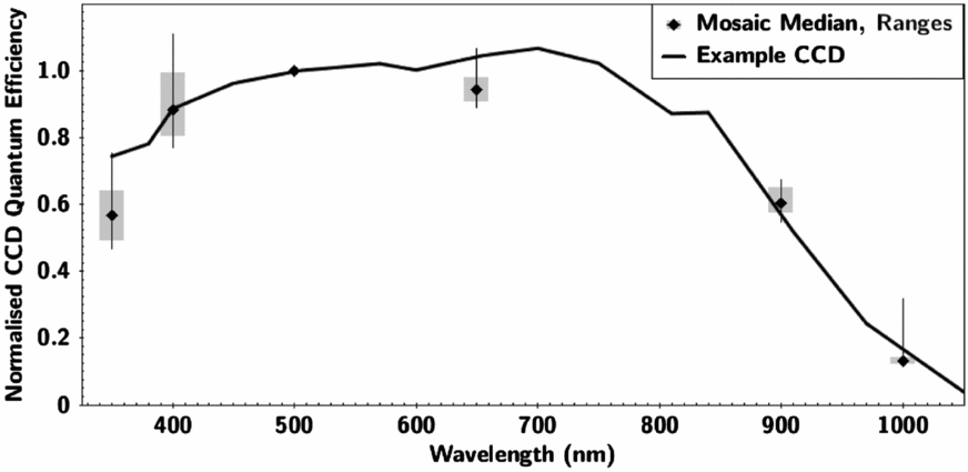
Figure 2. Quantum efficiency (QE) of the CCDs in the mosaic of the SkyMapper camera. Points indicate the median values after normalising to a common level at 500 nm wavelength, the grey bars indicate the 16th-to-84th-percentile range at each wavelength, and the thin errors bars indicate the minimum and maximum values. A more detailed QE curve for a single typical CCD is shown with a line. Different short-wavelength sensitivities are evident, which will lead to subtle variations in the uvg passbands.
3 THE SKYMAPPER SHALLOW SURVEY
The observations for the SkyMapper Southern Survey started after the end of the commissioning period, on 2014 March 15. The first year of observations was mostly dedicated to the Shallow Survey, where three visits were planned per field. Since the end of year 1, further Shallow Survey images have been collected in bright time around full moon, and we plan to reach five visits per field by the end of regular survey operations in the year 2020. Visits to the same field are scheduled to occur on separate nights, but no special constraints are applied, so the time separation between of any pair of visits on a given field varies from 20 h to over 500 nights; the median time between consecutive pairs is 10 nights.
Between 2014 April 29 and May 29, a fault in the filter mechanism forced us to observe with only one filter per night, and in this period SkyMapper observed an intense calibration programme instead of the Shallow Survey. On 2015 September 24, the helium compressor of the detector cooling system failed terminally. Since operations restarted with a new compressor two months later, the images show localised but strong electronic interference, which requires additional processing that is not yet available.
Hence, DR1 is focused on Shallow Survey data obtained in the first-compressor era 2014–15. During this period, several changes occurred that affect the image and calibration quality in DR1 in subtle ways, including a change in flatfield strategy implemented in 2014 November (see Section 4.3.2), and an early period until 2014 July 1 that is affected by certain detector artefacts (see Section 4.3.3).
DR1 includes 66 840 images after deselecting images of insufficient quality. The typical image properties are summarised in Table 1. Our quality cuts include
-
1. upper limits to the PSF FWHM (5 arcsec for griz and 6 arcsec for uv) and elongation (<1.4);
-
2. lower limit to the image ZPs (total instrument efficiency including atmospheric transmission) of roughly 24.5 mag, except 23.8 mag for v-band;
-
3. upper limit to the rms among the approximate ZPs derived from the calibrator stars within an image (only approximate, as these were applied before the DR1.1 recalibration), ranging from ~0.1 for z-band to ~0.2 mag for u-band;
-
4. upper limits on the background level to limit sky noise;
-
5. the number of well-measured calibrator stars in a frame needs to be at least 10 before a final clipping of outlier ZPs.
The median FWHM of the PSF among all DR1 images ranges from 2.3 to 3.1 arcsec from z-band to u-band, and the median PSF elongation is 1.12 independent of filter. Most images of the Shallow Survey are read-noise limited as the median sky background is less than 100 counts, except for the z-band images that are mostly background limited. The median airmass of observations is 1.11, but a tail to airmass 2 is unavoidable given that the sky coverage includes the South Celestial Pole.
The image ZPs are largely around 25.5 mag, with the exception of the shallower v-band. The ZPs show long-term drifts towards lower efficiencies until the mirrors were cleaned on 2015 May 5, resulting in an improvement by ~0.35 mag. Most image ZPs for a given filter scatter within less than 0.1 mag rms at a given calendar epoch, but some nights with bad weather produce tails with higher atmospheric extinction; the fraction of images with ZPs that are shallower by over 0.3 mag than the median ZP noted in Table 1 increases monotonically with light frequency from 5% in z-band to 12% in u-band.
Gaps between the CCDs in the detector mosaic imply that some sky coordinates are imaged less frequently than suggested by the number of field visits. Overlaps between neighbouring fields, however, mean that areas close to the field perimeters are observed many more times. The objects in the master table have visit numbers ranging mostly from 0 to 5 depending on filter, field, and coordinate, but the tail reaches up to 17 visits in g- and r-band, and, exceptionally, 35 visits in u-band. In z-band, e.g., the mean number of visits per object is 2.31, and about 1% of objects have more than five visits. Overall, the mean number of visits per object ranges from 2.0 in v-band to 2.8 in g-band.
Furthermore, objects might fall on bad pixels, which is ignored when computing the number of visits. Instead, these objects appear in the catalogues with flags indicating the presence of bad pixels. Every image has an associated mask image that combines globally bad pixels with frame-specific bad pixels. Globally, bad pixels are identified by a combination of algorithmic and manual processes and account for 0.31% of the pixels in each image. Frame-specific bad pixels include, e.g., pixels affected by cross-talk from saturated pixels in an associated amplifier (see Section 4.1.4).
The DR1 coverage map of the Southern sky (Figure 3) shows some areas with missing data: these include (1) regions that were not yet visited in good-quality conditions, which is the most common reason off the Galactic plane, and (2) regions that lack well-measured and reliable calibrator stars, which is the most common reason close to the Galactic plane. In DR1, photometry is heavily compromised by stellar crowding, lowering the number of cleanly measured (isolated) stars in dense star fields. This problem will overcome in future releases. Also, our photometric calibration source (see Section 4.5.2) contains areas where star colours are inconsistent with the expected stellar locus by more than 0.2 mag and those areas are not included in DR1.1, although they were part of DR1.0.
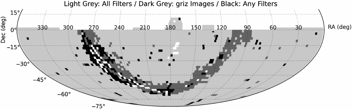
Figure 3. Sky coverage of the SkyMapper Southern Survey Data Release 1 (SMSS DR1): Most of the Southern hemisphere has been covered and calibrated in good conditions in all six passbands (light grey), but some fields along the Galactic plane have only data for griz in DR1 (dark grey), while fields without complete griz coverage are shown in black and fields without data are left white.
Within images, we note significant PSF variations caused by a curved focal plane, so they appear most pronounced in good seeing. We generally attempt to minimise the PSF variations by putting best focus not into a point in the centre, but into a ring. The PSF then deteriorates mildly towards the centre and moderately towards the corners. However, due to focus drifts at the telescope, the ring of best focus will breathe and cause varying patterns of deterioration. Figure 4 shows an example of an i-band image obtained in good seeing, where the PSF FWHM varies from 1.2 to 1.8 arcsec. In other images, we see e.g., variations from 2.8 to 3.5 arcsec, but a thorough investigation is beyond the scope of this paper. As we describe in Section 4.5.1, we compensate for PSF variations in the point-source photometry by constructing a 1D-PSF photometry estimate based on a sequence of aperture magnitudes and their trends across any individual image.
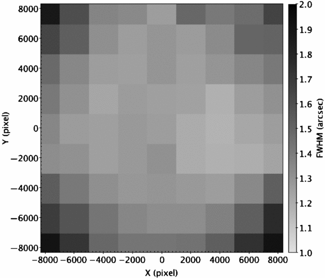
Figure 4. Map of the PSF FWHM across an i-band image taken in good seeing: due to a curved focal plane the FWHM ranges from 1.2 to 1.8 arcsec.
In DR1, we do not yet include any illumination correction to remove deviations of the measured flatfield from the true sensitivity pattern. A first analysis of illumination correction maps suggests that these correction are below ±1% on 90% of the mosaic area in all six filters. However, these corrections can reach up to 5% in the very corners of the image. As a result, a small fraction of objects situated close to field corners could be imaged under varying illumination conditions that are presently not accounted for. This effect will be corrected in future releases. Some images contained in the release are affected by dome vignetting, which causes a moderately high rms of the ZP estimate due to the changing collecting area across the field of view.
4 SCIENCE DATA PIPELINE
The images taken by SkyMapper are processed through the SDP, which utilises a PostgreSQLFootnote 2 database to semi-autonomously oversee the ingestion of each mosaic image, control the creation of the required calibration frames, produce reduced images, and perform photometric measurements and calibration (Luvaul et al. Reference Luvaul, Onken, Wolf, Smillie, Sebo, Lorente and Shortridge2015; Wolf et al. Reference Wolf, Luvaul, Onken, Smillie, White, Lorente and Shortridge2015). The flow of the SDP is outlined in Figure 5 and the sections below.
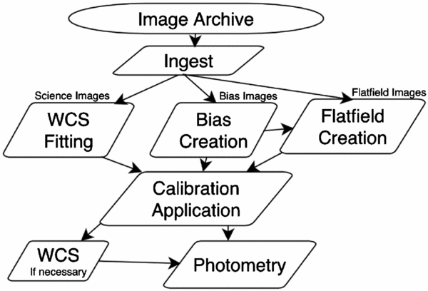
Figure 5. Flow chart of the steps in the Science Data Pipeline.
4.1. Ingest
Images from the telescope are transferred each morning via ethernet to long-term storage at the National Computational Infrastructure (NCI) located on the ANU campus. When a night is ready to be processed by the SDP, the data is moved from the NCI image archive to a local disk, and the individual images are then ingested into the SDP, which reorganises the 64 extensions of the FITS file (one per amplifier) into 32 separate FITS images (one per CCD). Preliminary quality assurance (QA) checks are performed to eliminate bad images from further processing. The initial processing during the ingest phase includes: suppression of interference noise; identification of pixels subject to saturation or blooming; overscan subtraction; correction for cross-talk; creation of image masks; and flipping the image axes to restore the on-sky orientation.
4.1.1. Interference noise
The SkyMapper detectors are subject to an intermittent, high-frequency source of interference, which imposes a strong sinusoidal pattern on the images with a wavelength between 6 and 7 pixels. The phase and amplitude can vary from row to row in an image, so each row read out by each amplifier is corrected individually by fitting a sine curve. In rare cases, the procedure does not adequately remove the pattern from a given row. The mean amplitude of the subtracted sine curve was 4.4 counts. An example of the interference noise and its removal are shown in Figure 6.
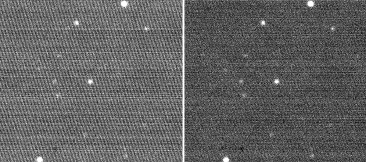
Figure 6. Left: Interference noise that appears intermittently in SkyMapper images, with amplitudes and row-to-row phase shifts that vary within a single readout. The wavelength along each row is between 6 and 7 pixels. We obtain a sinusoidal fit to each row, which is then subtracted to remove the interference. Right: The same image after removal of the fit to the noise. Residual row-to-row variations in the bias are removed by a separate step.
4.1.2. Saturated and bloomed pixel identification
For all image types except bias frames, we run Source Extractor (version 2.19.5; Bertin & Arnouts Reference Bertin and Arnouts1996) with a configuration designed to pick up heavily saturated sources: detection threshold of 58 000 counts and minimum area of 25 pixels. This identifies very bright sources as well as the surrounding pixels that are affected by blooming, and these are treated specially in the cross-talk correction (Section 4.1.4).
4.1.3. Overscan correction
Because the bias level has less structure in the post-scan regions (towards the centre of each CCD) than the pre-scan regions (Section 4.1.5), the post-scan level in each row is used for the overscan correction. Taking the last 45 pixels in the 50-pixel post-scan region, the set of pixels is 3σ-clipped until convergence, and the median of the resulting distribution is subtracted from the row.
4.1.4. Amplifier cross-talk and ringing
The SkyMapper mosaic is subject to electronic cross-talk between its 64 amplifiers. The most severe cross-talk, and the only one treated by the current version of the SDP, occurs between adjacent amplifiers on the same CCD, with a fractional amplitude of ~5 × 10⁻⁴. However, in the presence of fully saturated pixels, other amplifiers can display cross-talk artefacts (switching between negative and positive counts on alternative amplifiers) with fractional amplitudes as high as 1 × 10⁻⁴ or about seven counts. Fully saturated pixels also induce amplifier ringing, where the next non-saturated pixel read out has 0 counts and the subsequent two pixels have severely suppressed count levels. Figure 7 shows examples of these behaviours.
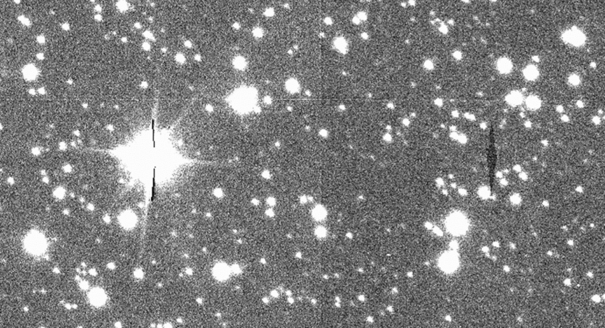
Figure 7. Example image showing cross-talk between amplifiers, visible as depressed counts opposite the bright star on the left, and amplifier ringing, visible as dark regions immediately adjacent to the pixel blooming associated with the bright star on the left.
Cross-talk between the two amplifiers on the same CCD is corrected by subtracting a second-order polynomial in the count level, with an additional subtractive component for the counterpart of a fully saturated pixel. The correction is made in a single pass through each CCD, beginning with the left-hand amplifier and then correcting the right-hand amplifier.Footnote 3
The pre- and post-scan pixels are then trimmed from both amplifiers of a given CCD, and the two amplifiers are stitched together into a single FITS image. Finally, the images and masks are flipped in the x-direction to restore the on-sky orientation.
4.1.5. Detector bias
The SkyMapper detectors exhibit no significant fixed-pattern bias structure, but there are two kinds of row-oriented, time-variable bias features that are seen. The first is a slow change in the bias level along the row, with the spatial scale of the variation increasing from the pre-scan towards the post-scan in each amplifier. The variations can be well modelled by a principal components (PCs) analysis described in Section 4.3.1.
The second kind of bias features are known as ‘fingers’, and consist of regions of suppressed bias level near the edges of the frame. Most of the SkyMapper CCDs show some amount of this behaviour, but in a small number of CCDs, a fraction of the rows (which change from readout to readout) have the suppressed bias level extending from the pre-scan region into the on-sky portion of the detector. The amplitude of the bias offset is typically 20 counts, with a distribution that extends to ~40 counts, and the bias makes a sharp transition back to the nominal level for the rest of the row. These features remain uncorrected in DR1.
4.1.6. Mask creation
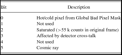
Image-specific masking augments the global bad pixel mask. We identify saturated pixels using a threshold of 55000 counts. The fully saturated pixels and the three neighbouring pixels subject to amplifier ringing are all masked with a saturation flag. Pixels subject to cross-talk from saturated pixels in the other amplifier on the same CCD are masked with a separate flag. Finally, as described in Section 4.4, pixels in which cosmic rays have been identified and corrected are flagged. The various image-mask flags are described in Table 2.
Table 2. Meanings of image mask flags.
Very bright stars leave some strong and curiously shaped optical reflections in the images, which have not been removed (see Figure 8 for an example).

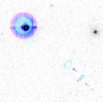
Figure 8. Optical reflections from very bright stars (here, Antares) are not removed from images in DR1. This image is an inverted-colour image from the SkyMapper SkyViewer.
4.2. Astrometry
The astrometric solutions for the survey images are tied to the fourth U.S. Naval Observatory CCD Astrograph Catalog (UCAC4; Zacharias et al. Reference Zacharias, Finch, Girard, Henden, Bartlett, Monet and Zacharias2013). The 32 CCDs are each run independently through the solve-field program from the Astrometry.net software suite (version 0.43; Lang et al. Reference Lang, Hogg, Mierle, Blanton and Roweis2010), using a set of UCAC4 index files, to generate tangent-plane World Coordinate System (WCS) solutions. Each CCD for which solve-field succeeds is then run through Source Extractor to derive (x, y) pixel positions and RA, Dec values for each source, as well as to calculate the median seeing and elongation values for the CCD (using Source Extractor parameters FWHM_IMAGE and ELONGATION). For each source in the image, the closest-matching RA, Dec position from the UCAC4 catalogue is taken as the true position,Footnote 4 and we then fit a Zenithal Polynomial (ZPN) projection (see Calabretta & Greisen Reference Calabretta and Greisen2002) to the pixel+coordinate sets using a fixed curvature term of PV2_3 = 3.3, which was determined by an independent fit to a well sampled mosaic image. The ZPN solution provides a good fit to the radial distortions in the SkyMapper focal plane, but the ZPN formalism is not understood by several of the software tools utilised by the SDP. Hence, the ZPN solution is then transformed into a TPV projection (tangent plane with generalised polynomial distortion)Footnote 5 , which can be understood by the software packages from AstrOmaticFootnote 6 (e.g., SExtractor, SWarp, and PSFEx).
After all 32 CCDs have been analysed, two QA tests are performed: the plate scale near the middle of each CCD is required to be between 0.487 and 0.507 arcsec (0.483 and 0.507 arcsec for the four corner CCDs); and the offset from the middle of the CCD to the middle of one of the central CCDs is required to be within 10 arcsec of the nominal value. Later, a third test is performed on the WCS solutions, requiring that the corner-to-corner lengths of each CCD are within 2 arcsec of a reference value, where the reference is dependent on the CCD position within the mosaic, the filter used in the observation, and the fractional Modified Julian Date (MJD). The dependence on the fractional MJD, which contributes 0.5 arcsec of variation across the observed fractional MJD range, is thought to reflect temperature gradients in the Corrector Lens Assembly, which evolve as a night progresses. This final test ensures that the WCS solutions do not extrapolate to unrealistic representations of the sky in regions where there may be too few stars to constrain the fit.
Overall, 98.6% of mosaic images used in DR1 yield valid WCS solutions for all 32 CCDs, and amongst the few images that yield between 1 and 31 valid WCS solutions, the mean number is over 28. The success rate is lowest in the u- and v-filter with 96.7% each, because the density of stars bright enough to match to UCAC4 is the lowest. Whenever a valid WCS solution is not available for a CCD, it has further calibrations applied as normal, after which a second attempt is made to obtain a WCS solution.
As an indicator of the quality of our WCS solutions in DR1, we show the median offset distances between the sources in our DR1 master table and the nearest source in Gaia DR1 (Lindegren et al. Reference Lindegren2016) as a function of RA and Dec in Figure 9. The overall median offset (restricted to distances less than 10 arcsec) is 0.16 arcsec and the [10%, 90%] range is [0.06 arcsec, 0.45 arcsec]. For cleanly detected objects with r-band magnitudes between 9 and 14 mag, the median offset is 0.12 arcsec, or about 1/20th of the typical PSF FWHM.
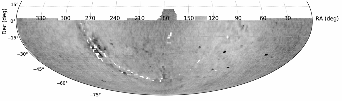
Figure 9. Median positional offset between the DR1 sources and the closest match from the Gaia DR1 catalogue, as a function of Right Ascension and Declination. The grayscale ranges from 0 (white) to 0.5 arcsec (black). The overall median offset is 0.16 arcsec.
4.3. Calibration data
The individual bias and flatfield exposures are combined into a series of master frames with variable durations of validity. Hard boundaries on the input frames considered for each master calibration frame are imposed at each instance of detector warming (when we find subsequent rapid evolution of the flatfield shape), as well as at any other significant change to the image properties, such as modification of detector voltages (Section 4.3.3), changes to flatfield position angles (PAs), or cleaning of the telescope optics.
4.3.1. Bias creation
The typical observing night includes the acquisition of 10 bias exposures, which are used to generate the master bias frame valid for the night. In cases when fewer than 10 biases were obtained, the adjacent nights are considered. In practice, all master bias frames have at least 10 inputs, and for most nights, all inputs come from the night in question. The maximum range of input nights is 8.
From the input biases selected, the master bias frame is created as the mean image, while rejecting outliers that are 50 counts above or below median for each CCD. Pixels from the global bad pixel mask are set to 0 counts. The master bias is then subtracted from each of the input biases, which then are used to generate the night-specific PCs for the residual bias shape along each row (using the scikit-learn Python module; Pedregosa et al. Reference Pedregosa2011). We treat the two halves of the CCD separately to account for the differing behaviour between amplifiers, and for each amplifier, we compute the mean and next 10 PCs of the per-row bias pattern. In addition, we derive limits for the allowable PC amplitudes when later fitting the science frames. The limits are set to trim off the most extreme 0.25% of values from either end of the bias frame PC amplitude distribution.
4.3.2. Flatfield creation
The approach for considering potential inputs to a master flatfield differs from the bias frames in several respects. To minimise the effect of spurious variations in the observed flatfield images due to, e.g., clouds, all flatfield images within ±10 nights are considered, except where that range encounters one of the hard boundaries between calibration windows. This results in a median range of 17 nights. The potential inputs are then trimmed of any inputs in which any of the 32 CCDs exceeds certain tolerances in terms of the CCD count level relative to the mean of the central eight CCDs.Footnote 7 The tolerances are set to ±10% of the mean count ratio defined over a long time baseline and specific to each filter, PA, and twilight (evening/morning). The median number of inputs to the master flatfields ranges from 65 (z-band) to 85 (v-band).
The algorithm employed for flatfield creation then depends on whether the inputs were obtained with fixed PA (0°; from the start of the survey through 2014 November 19) or with opposing-pair PAs. On 2014 November 25, we started taking flatfields in rotated pairs to capture and eliminate the gradient in sky brightness across our large field of view.Footnote 8
In the fixed-PA era, the input flats are first bias-corrected using the master bias frame.Footnote 9 For most master flatfields, the inputs are median-combined with 3σ-clipping, including scale factors defined as the inverses of the mean count levels in the central eight CCDs of each input (to preserve the relative scaling of each CCD within the mosaic). For one master flat in r-band, there was only three input exposures available, and in that case, we took the minimum value at each pixel as a way of rejecting any astronomical sources present in the input images.
For the opposing-pair era, the potential input frames are grouped by PA, and a similar tolerance-testing procedure is applied as in the fixed-PA era. Within each PA, the remaining inputs are median-combined after rescaling the counts by the mean of the central eight CCDs. For the opposing PAs within each twilight, the PA-medians are then mean-combined with equal weighting. Finally, the twilight-means are combined in a weighted mean, where the weights are taken as the number of contributing input frames, resulting in the master flatfield.
In both the fixed-PA and opposing-pair eras, pixels from the global bad pixel mask are set to a value of 1.
4.3.3. Detector ‘tearing’
In early 2014, it was discovered that all 32 of the CCDs exhibited curvilinear features in which approximately 5% of the counts appeared to be shifted to neighbouring columns. An example is shown in Figure 10. The position of these features differed from amplifier to amplifier and changed position from image to image, and hence we leave them uncorrected in DR1. The features were eventually identified as being instances of ‘tearing’ (cf. Doherty Reference Doherty2013; Rasmussen Reference Rasmussen2014) and were traced to the detector bias voltage settings being used at the time. From 2014 July, an updated configuration, modelled on the settings used by the European Southern Observatory, eliminated the features from subsequent SkyMapper images. However, the relative-strength nature of the tearing means that in DR1 the features may be visible in flatfields with few input frames or in high-background images taken prior to 2014 July.
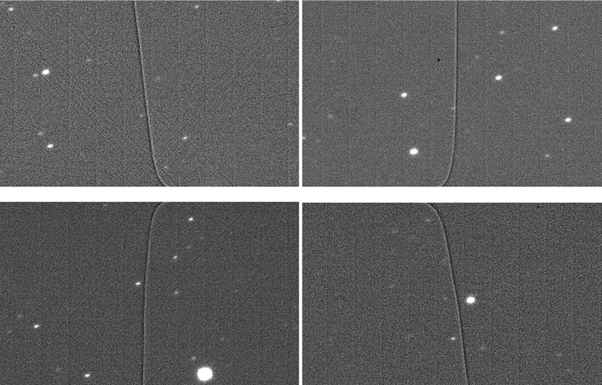
Figure 10. Detector ‘tearing’ on four amplifiers across four CCDs from an r-band flatfield image from UT 2014 March 31. The amplitude of the features is approximately 5% of the nominal count level. The position of the features varied with amplifier and with each image. Modifications to the detector bias voltages eliminated the features from 2014 July onward.
4.4. Application of calibrations
For each CCD frame of a science image, we first subtract the associated master bias frame. Then we prepare the science frame for PC-fitting by creating a background map using SExtractor and identify sources in the image for masking from the fit. After subtracting the background, we fit unmasked pixels with a weighted least-squares algorithm, using the PCs associated with the master bias for that night (Figure 11). Again, each half of the CCD is treated separately. The number of PCs included in the fitting procedure is determined by the fraction of the pixels in the row that remain unmasked: all 10 PCs for at least 25% unmasked; five PCs if 10–25% of the row is unmasked; one PC if 2–10% of the row is unmasked; and no fitting is performed if less than 2% of the row is unmasked.
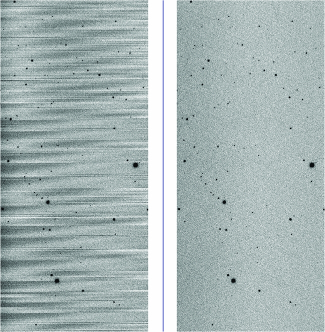
Figure 11. Example of bias residuals after traditional overscan correction used in the SkyMapper Early Data Release (EDR, left) vs. PCA model-based bias removal used in DR1 (right).
After the bias PCA treatment, the master flatfield is divided out.
Next, cosmic rays are detected and removed from the science frames using the lacosmicx software package,Footnote 10 a fast Python implementation of the L.A.Cosmic routine (van Dokkum Reference van Dokkum2001). Each amplifier is treated separately to allow for the use of specific read noise settings. From over 7 000 bias frames taken during the DR1 period, we determine the read noise in each frame, and determine for each amplifier a mean level and an rms variation over time. To avoid removal of spurious cosmic rays from uncorrected interference noise in higher noise frames, we use a high fiducial value for the read noise, setting it to 〈RON〉 + 3σRON + 1 counts for each amplifier. The range of input read noise values is 7.36–17.04, with a median of 9.95 counts. The saturation level is set to 60 000 counts, with a Laplacian-to-noise limit of 6σ and a fractional detection limit for neighbouring pixels of 1.35σ. The image mask is provided as an input to lacosmicx in order to avoid detecting known bad pixels.
We then still observe residual differences in the sky level between the two halves of each CCD due to non-linearity at low count rates. We call SExtractor again to create a background map for each half of the image. From the two background maps, the median value for seven columns near the centre of the CCD (omitting the three columns closest to the middle) are compared, and the difference is then applied as an additive offset to all pixels in the lower of the two halves.
Next, an existing WCS solution is inserted into the image header. The pixel values are then converted to 16-bit integers, with a BZERO value of 32 668 and a BSCALE value of 1, to give a resulting count range of −100 to 65 435 (preserving the noise near zero counts), and the images and masks are compressed using the lossless fpack FITS Image Compression Utility (Pence, Seaman, & White Reference Pence, Seaman and White2009) from the CFITSIO library.Footnote 11
Any images for which the raw image could not generate a WCS solution are tried again after the calibrations have been applied. If still no WCS could be obtained, the CCD is discarded for further analysis.
4.5. Photometry
For any mosaic image in which at least one CCD has yielded a valid WCS solution, the suitable CCDs are then run through our photometry stage.
First, SExtractor is run on each CCD. We use a detection threshold of 1.5σ, the default (pyramidal) filtering function, a minimum area of 5 pixels, a minimum deblending contrast of 0.01, employ a local background estimate, utilise cleaning around bright objects, and measure photometry in a series of apertures (diameters of 4, 6, 8, 10, 12, 16, 20, 30, 40, and 60 pixels). We provide SExtractor with the image-specific mask as a Flag image and a version of the global bad pixel mask as a Weight image. The parameters measured by SExtractor are shown in Table A1 of the Appendix.
4.5.1. Aperture corrections
We adopt the 30-pixel-diameter (≈15 arcsec) photometry as the reference aperture for our aperture corrections. For each of the apertures smaller than 15 arcsec, we select candidate sources (those with positive fluxes, no flagged pixels from the mask, SExtractor flags less than 4, a semi-minor axis length of at least one pixel), where we progressively relax constraints on the flux errors and the CLASS_STAR values if fewer than eight stars on the CCD meet the criteria. Ultimately, if at least five stars are available, the ratio of fluxes between the aperture in question and the reference aperture are fit with a 2-D linear plane, which was found to sufficiently account for any spatial variation in the aperture corrections across a single CCD. The fit is revised through four passes of 2.5σ-clipping, and the final correction parameters are then applied to all stars on the CCD to yield corrected aperture magnitudes (i.e., predicted 15 arcsec aperture magnitudes based on the smaller apertures). The errors on the corrected fluxes are calculated by square adding the original flux errors with the RMS around the final planar fit. In cases when fewer than six stars remain unclipped, no gradient is fit and the median aperture correction is adopted for the CCD.
The predicted 15 arcsec aperture magnitudes from the seven smallest apertures are then used to estimate a ‘PSF’ magnitude and error, taken as the weighted mean of the inputs and the error on the weighted mean. The χ2 value from the fit is also estimated as a way of distinguishing between point sources and other spatial profiles (cosmic rays or extended objects). Note, that these ‘PSF’ magnitudes will be affected by nearby neighbours that contribute flux to the 15 arcsec aperture.
4.5.2. Zero-point calibration
For SkyMapper DR1, the ZP calibration is referenced to the AAVSO Photometric All Sky Survey (APASS DR9; Henden et al. Reference Henden, Templeton, Terrell, Smith, Levine and Welch2016) and 2MASS. From APASS DR9, we select suitable calibrator stars with clean flags,Footnote 12 magnitude errors below 0.15 and magnitudes in the ranges of g = [11.5, 16.5] and r = [10.5, 16]. From 2MASS, we select stars with clean flags, no neighbours within 10 arcsec and K < 13.5. This leaves approximately 12.8 million APASS DR9 sources and 2.5 million 2MASS sources at δ < +30°. Then we compute predicted magnitudes in all SkyMapper filters with a method trained on photometry from the first data release of the Pan-STARRS1 3π Steradian Survey (PS1; Chambers et al. Reference Chambers2016; Flewelling et al. Reference Flewelling2016; Magnier et al. Reference Magnier2016).
We first dereddened stars in all three catalogues using the reddening maps by Schlegel, Finkbeiner, & Davis (Reference Schlegel, Finkbeiner and Davis1998; hereafter, SFD) and bandpass coefficients derived from a Fitzpatrick (Reference Fitzpatrick1999) extinction law. Then we used a large sample of stars that are well-measured in all three catalogues to fit linear relations predicting PS1 magnitude from APASS and 2MASS. As a final step, we apply a linear PS1-to-SkyMapper transformation that was derived using the filter curves of PS1 and SkyMapper together with the unreddened F- and G-type main-sequence and sub-giant stellar templates from Pickles (Reference Pickles1998).
From PS1, we find that trends of mean stellar colour with reddening are minimised if we adopt for the mean reddening of the average star, a prescription of
 $$\begin{equation*}
\frac{\text{d}E(B-V)_{\rm eff}}{\text{d}E(B-V)_{\rm SFD}} = \left\lbrace \begin{array}{@{}l@{\quad }l@{}}0.82, & \text{if}\ E(B-V)_{\rm SFD}<0.1 \\
0.65, & \text{otherwise}. \end{array}\right.
\end{equation*}$$
$$\begin{equation*}
\frac{\text{d}E(B-V)_{\rm eff}}{\text{d}E(B-V)_{\rm SFD}} = \left\lbrace \begin{array}{@{}l@{\quad }l@{}}0.82, & \text{if}\ E(B-V)_{\rm SFD}<0.1 \\
0.65, & \text{otherwise}. \end{array}\right.
\end{equation*}$$
Schlafly & Finkbeiner (Reference Schlafly and Finkbeiner2011) had already found that the SFD maps overestimate reddening on average and suggest to generally scale them by a factor 0.86. We also find that we need to reduce more strongly the reddening at E(B − V)SFD > 0.1, and fit a coefficient in order to remove trends of the mean star colour with reddening. We find the same coefficient 0.65 as previously suggested by Bonifacio, Monai, & Beers (Reference Bonifacio, Monai and Beers2000) for stars of V = [11, 15]. This scaling probably accounts for the fact that a fraction of the stars reside in front of some of the dust that contributes to the IR emission in the SFD maps.
We estimate reddening coefficients for our filters using a Fitzpatrick (Reference Fitzpatrick1999) extinction law with R V = 3.1. This appears to best match the empirical bandpass coefficients found by analysing trends in the observed colours of stars (Schlafly & Finkbeiner Reference Schlafly and Finkbeiner2011) and QSOs (Wolf Reference Wolf2014) with reddening. Our mean bandpass reddening coefficients R band are listed in Table 1, and while they apply strictly only to flat spectra, as R band depends on the object SED, this effect is mostly relevant in the u-band.
We restrict calibrator stars to certain colour ranges after de-reddening in order to ensure sufficient linearity of the colour transformation. For calibrating iz images, we use stars with (J − K)0 = [0.4, 0.75] and (g − r)0 = [0.2, 0.8]; for gr images, we require only (g − r)0 = [0.2, 0.8] and for uv images, we use (g − r)0 = [0.4, 0.8].
Final SkyMapper AB magnitudes are estimated from APASS AB and 2MASS Vega magnitudes using
 $$\begin{eqnarray*}
u_2 & = & g_{\rm AP} + 0.622 + 1.757(g-r)_0 + 0.953 E(B-V)_{\rm eff}; \\
u_1 & = & g_{\rm AP} + 0.575 + 2.050(g-r)_0 + 1.002 E(B-V)_{\rm eff}; \\
v & = & g_{\rm AP} + 0.033 + 2.240(g-r)_0 + 0.734 E(B-V)_{\rm eff}; \\
g & = & g_{\rm AP} - 0.010 - 0.295(g-r)_0 - 0.306 E(B-V)_{\rm eff}; \\
r & = & r_{\rm AP} - 0.003 + 0.042(g-r)_0 + 0.014 E(B-V)_{\rm eff}; \\
i & = & J_{\rm 2M} + 0.270 - 0.060(g-r)_0 + 0.060 E(B-V)_{\rm eff} \\
&& +\, 0.31(r-J)_0 + 0.207(g-J)_0 + 0.062(J-K)_0; \\
z & = &J_{\rm 2M} + 0.550 + 0.062(g-r)_0 + 0.510 E(B-V)_{\rm eff} \\
&& +\, 0.880(J-K)_0.
\end{eqnarray*}$$
$$\begin{eqnarray*}
u_2 & = & g_{\rm AP} + 0.622 + 1.757(g-r)_0 + 0.953 E(B-V)_{\rm eff}; \\
u_1 & = & g_{\rm AP} + 0.575 + 2.050(g-r)_0 + 1.002 E(B-V)_{\rm eff}; \\
v & = & g_{\rm AP} + 0.033 + 2.240(g-r)_0 + 0.734 E(B-V)_{\rm eff}; \\
g & = & g_{\rm AP} - 0.010 - 0.295(g-r)_0 - 0.306 E(B-V)_{\rm eff}; \\
r & = & r_{\rm AP} - 0.003 + 0.042(g-r)_0 + 0.014 E(B-V)_{\rm eff}; \\
i & = & J_{\rm 2M} + 0.270 - 0.060(g-r)_0 + 0.060 E(B-V)_{\rm eff} \\
&& +\, 0.31(r-J)_0 + 0.207(g-J)_0 + 0.062(J-K)_0; \\
z & = &J_{\rm 2M} + 0.550 + 0.062(g-r)_0 + 0.510 E(B-V)_{\rm eff} \\
&& +\, 0.880(J-K)_0.
\end{eqnarray*}$$
Because of the red leak in the SkyMapper u-band, atmospheric extinction makes the filter transformations airmass-dependent (see Figure 1). We calculate predicted u-band magnitudes for airmasses of 1 and 2, and interpolate between those based on the airmass of each exposure.
For each SkyMapper source having a positive 15 arcsec-aperture flux, a 15 arcsec-aperture magnitude error less than 0.04 mag, SExtractor FLAGS < 4 (i.e., not saturated), NIMAFLAGS = 0 (i.e., no masked pixels within the isophotal area), and semi-minor axis size of at least 1 pixel, we find the closest match on the sky from the sample of calibrator stars, with a maximum positional difference of 10 arcsec.
We compute the differences in observed and predicted magnitudes for each star on all available CCDs for the mosaic image, along with the whole-of-mosaic (x, y) positions for those stars (adopting the median CCD-to-CCD offsets from ~10 000 images with clean WCS solutions). With the positions and ZP estimates from the entire mosaic, we then simultaneously fit for linear gradients in x and y, in order to take atmospheric extinction gradients across the large field of view into account.
We perform four passes of 2.5σ-clipping to determine the final ZP gradient, and fix the gradients to be zero when five or fewer stars remain unclipped. The resulting ZP plane is then applied to the magnitudes for all sources detected in the mosaic. The RMS around the final ZP fit is recorded, but not applied to the individual magnitude errors. Most images in DR1 have between 300 and 1 000 calibrator stars per frame that are used for the ZP calibration, and in all bands at least 95% of frames have more than 100 calibrator stars.
We adjust all u-band magnitudes globally 0.05 mag brighter, which makes our measurements consistent with SkyMapper u-band predictions derived from measured PS1 g- and r-bands (see Section 5.1 for details).
Prior to uploading the photometry into the database, we perform a small amount of cleaning. Because SExtractor does not provide error estimates for the PA, we adopt the PA error used for the Chandra Source Catalog:
 $$\begin{eqnarray*}
e_{\rm PA} &=& {\rm atan2}((b+e_b),(a-e_a))\\
&& -\, {\rm atan2}((b-e_b),(a+e_a)),
\end{eqnarray*}$$
$$\begin{eqnarray*}
e_{\rm PA} &=& {\rm atan2}((b+e_b),(a-e_a))\\
&& -\, {\rm atan2}((b-e_b),(a+e_a)),
\end{eqnarray*}$$
where a and b are the semi-major axis and semi-minor axis lengths, respectively, and e a and e b are their errors;Footnote 13 and we impose a minimum PA error of 0.01°. We also impose magnitude error floors of 0.0033 mag, and we remove sources having negative fluxes in their 30 arcsec apertures.
4.5.3. Catalogue distill
In a final step, we distill the photometry table with one row per individual detection into a master table with one entry per unique astrophysical object, using only detections that are not affected by bad flags (FLAGS <8). Before the matching, we set the flag with bit value 512 for all detections where any of MAG_APC05, MAG_APR15, or MAG_PETRO is fainter than 19 mag. We also mark unusually concentrated sources such as possible cosmic rays by setting the flag with bit value 1 024, and identify these using MAG_APC02−MAG_APR15 <−1 AND CHI2_PSF >10. We mark sources in the vicinity of bright stars by setting the flag with bit value 2 048 as these are either spurious or their photometry is affected by scattered light. We consider the environments of stars with V < 6 in the Yale Bright Star Catalogue (Hoffleit Reference Hoffleit and Hoffleit1964; Hoffleit & Warren Reference Hoffleit and Warren1995) and of stars with g phot < 8 from Gaia DR1, marking all sources within radii of 10−0.2V or 10 − 0.2g phot degrees, respectively.
Within each passband, we then position-match detections across different images into groups. We first classify every detection as either a primary or secondary detection, using the latter label when another detection with a higher central count level (FLUX_MAX) is found on any image within a matching radius of 2 arcsec. We then associate every secondary detection with the nearest primary detection, which can be over 2 arcsec away to accommodate chains of detections. Within each group, we combine positions and shapes as unweighted averages, but combine PSF and PETRO photometry as inverse-variance weighted averages. FLAGS are BIT_OR-combined, NIMAFLAGS are summed up, and from CLASS_STAR and FLUX_MAX we pick the largest value.
Next, we merge the per-filter averaged detections between the six filters with a similar procedure. At this stage, however, positions are averaged by weighting them with inverse variance, while shapes, flags, and other columns are combined as with the per-filter merging. Most of the time, this process finds only one source per filter (or none) to combine into a unique astrophysical object. Sometimes, however, one astrophysical parent source is associated with two or more child sources in some filter, e.g., a single bright red child source might lie in between two separated faint blue child sources, and be close enough to all be merged into one single parent. In these cases, we attempt to combine the fluxes of the child sources into a total flux, although at this point we do not trust the resulting photometry. Certainly, the PSF photometry can end up counting flux multiple times and thus overestimate the total brightness of a source with multiple children. We always note the number of children per band for each object in the master catalogue, so that it is easy to avoid those sources when selecting complete, photometrically clean samples.
The final master table is cross-matched with several external imaging catalogues, including APASS DR9, UCAC4, 2MASS, AllWISE (Wright et al. Reference Wright2010; Mainzer et al. Reference Mainzer2011), PS1 DR1, Gaia DR1, and the GALEX All-sky Imaging Survey (BCScat; Bianchi, Conti, & Shiao Reference Bianchi, Conti and Shiao2014), such that every entry in the SkyMapper table contains an ID pointer to the corresponding object in the external table. The master table is also cross-matched against itself to identify the ID and distance to the nearest neighbour of every source. The maximum matching radius for all cross-matches is 15 arcsec. In contrast, external spectroscopic catalogues are also cross-matched to the final master table, but such that the external table contains a pointer to the SkyMapper ID, because of the relatively small row numbers in the spectroscopic tables. The cross-matched spectroscopic catalogues include the 6dF Galaxy Survey (6dFGS; Jones et al. Reference Jones2004, Reference Jones2009), the 2dF Galaxy Redshift Survey (2dFGRS; Colless et al. Reference Colless2001), the 2dF QSO Redshift Survey (2qz6qz; Croom et al. Reference Croom, Smith, Boyle, Shanks, Miller, Outram and Loaring2004), and the Hamburg/ESO Survey for Bright QSOs (HES QSOs; Wisotzki et al. Reference Wisotzki, Christlieb, Bade, Beckmann, Köhler, Vanelle and Reimers2000). When using cross-match IDs, care needs to be taken to observe the distance column in order to pick only likely physically associated detections. Credible distance thresholds depend on the resolution of the external dataset, e.g., a larger value for AllWISE than for 2MASS, as well as on the epoch difference and proper motion in the case of nearby stars.
5 SURVEY PROPERTIES
5.1. Photometric comparison: SkyMapper vs. PanSTARRS1 DR1
First, we assess the internal reproducibility of measured SkyMapper ‘PSF’ magnitudes of point sources from repeat visits and find that it ranges from 8 mmag rms in griz-bands to 12 mmag in the uv-bands. For a comparison against external data, we chose to use Pan-STARRS1 DR1 and estimate magnitudes in SkyMapper bands from existing measurements in PS1 bands. After checking colour trends with magnitude, we restrict this comparison to calibrator stars that appear well-measured in both surveys, thus ensuring that the transformation from PS1 to SkyMapper bands is reliable.Footnote 14 We deredden the PS1 SED using the modified mean reddening E(B − V)eff specified in Section 4.5.2, and apply colour terms fitted on synthetic PS1 and SkyMapper photometry of Pickles (Reference Pickles1998) stars with luminosity class IV and V and colour range (g − r)0 = [0.2, 1.0]. We apply the following equations to transform measured PS1 griz magnitudes into SkyMapper magnitudes, using a de-reddened PS1 colour of (g − i)0 = g − i − 1.5 E(B − V)eff:
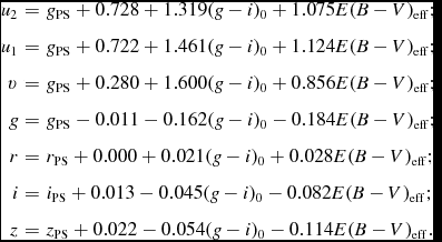 $$\begin{eqnarray*}
u_2 & = & g_{\rm PS} + 0.728 + 1.319(g-i)_0 + 1.075 E(B-V)_{\rm eff}; \\
u_1 & = & g_{\rm PS} + 0.722 + 1.461(g-i)_0 + 1.124 E(B-V)_{\rm eff}; \\
v & = & g_{\rm PS} + 0.280 + 1.600(g-i)_0 + 0.856 E(B-V)_{\rm eff}; \\
g & = & g_{\rm PS} - 0.011 - 0.162(g-i)_0 - 0.184 E(B-V)_{\rm eff}; \\
r & = & r_{\rm PS} + 0.000 + 0.021(g-i)_0 + 0.028 E(B-V)_{\rm eff}; \\
i & = & i_{\rm PS} + 0.013 - 0.045(g-i)_0 - 0.082 E(B-V)_{\rm eff}; \\
z & = & z_{\rm PS} + 0.022 - 0.054(g-i)_0 - 0.114 E(B-V)_{\rm eff}.
\end{eqnarray*}$$
$$\begin{eqnarray*}
u_2 & = & g_{\rm PS} + 0.728 + 1.319(g-i)_0 + 1.075 E(B-V)_{\rm eff}; \\
u_1 & = & g_{\rm PS} + 0.722 + 1.461(g-i)_0 + 1.124 E(B-V)_{\rm eff}; \\
v & = & g_{\rm PS} + 0.280 + 1.600(g-i)_0 + 0.856 E(B-V)_{\rm eff}; \\
g & = & g_{\rm PS} - 0.011 - 0.162(g-i)_0 - 0.184 E(B-V)_{\rm eff}; \\
r & = & r_{\rm PS} + 0.000 + 0.021(g-i)_0 + 0.028 E(B-V)_{\rm eff}; \\
i & = & i_{\rm PS} + 0.013 - 0.045(g-i)_0 - 0.082 E(B-V)_{\rm eff}; \\
z & = & z_{\rm PS} + 0.022 - 0.054(g-i)_0 - 0.114 E(B-V)_{\rm eff}.
\end{eqnarray*}$$
The g-band filter shows the most significant colour term, while the u- and v-band must be extrapolated from g, which is inherently less accurate. The v-band magnitude in particular also depends on metallicity and shows clear trends between the halo and disk population. Indeed, the motivation for the SkyMapper v-band is to act as a metallicity and surface gravity indicator for stars, and below we demonstrate the first step in our search for EMP stars (see Section 6.3).
In Figure 12, we show the difference between the measured and PS1-predicted SkyMapper photometry in histograms after binning in foreground reddening, as well as in sky maps. We restrict this comparison to the four non-extrapolated filters griz, and find an rms scatter in the magnitude difference of 23 mmag. The mean offset is generally less than 10 mmag, with the exception of a tail at higher reddening in z-band, where the median difference increases to 0.06 mag for E(B − V) = [0.5, 1.5]. The sky maps also show the bias in z-band towards low Galactic latitude where reddening tends to be higher. Apart from that the sky maps show low-level discontinuities at the SkyMapper field edges. SkyMapper fields are arranged in declination stripes with small overlaps in RA and Dec. However, additional passes of the Shallow Survey after the DR1 imaging period provide field overlaps to support a more homogeneous calibration.
Figure 12. Difference between SkyMapper magnitude as measured in DR1 and as predicted from PS1 magnitudes with bandpass transformations applied. This comparison is restricted to calibrator stars that are well measured and have reliable transformations. Top: histograms in bins of interstellar foreground reddening up to E(B − V) = 1.5. The bottom four panels show spatially resolved sky maps.
Despite the uncertainties introduced by extrapolating the SkyMapper u- and v-band, we can formally compare the photometry. Again we derive colour terms for SkyMapper u at airmass 1 and 2, although in this comparison, we use the median airmass of 1.11 to represent the whole comparison sample. We show the histograms of magnitude differences in Figure 13 and note that the rms scatter is 0.12 mag in both bands. After finding a mean offset of 0.05 mag in u we adjusted all our u-band magnitudes globally 0.05 mag brighter. We assume that this offset has originated from our calibration procedure, where we extrapolated the APASS DR9 gr photometry to the SkyMapper u-band. Even though we see slight offsets in v-band and a ~0.05 mag difference between regions of reddening less than E(B − V) = 0.1 and those with more reddening, we do not correct these. The shift with reddening is likely to be a metallicity effect, where halo and disk stars are expected to have different v − g colours by roughly the observed amount.
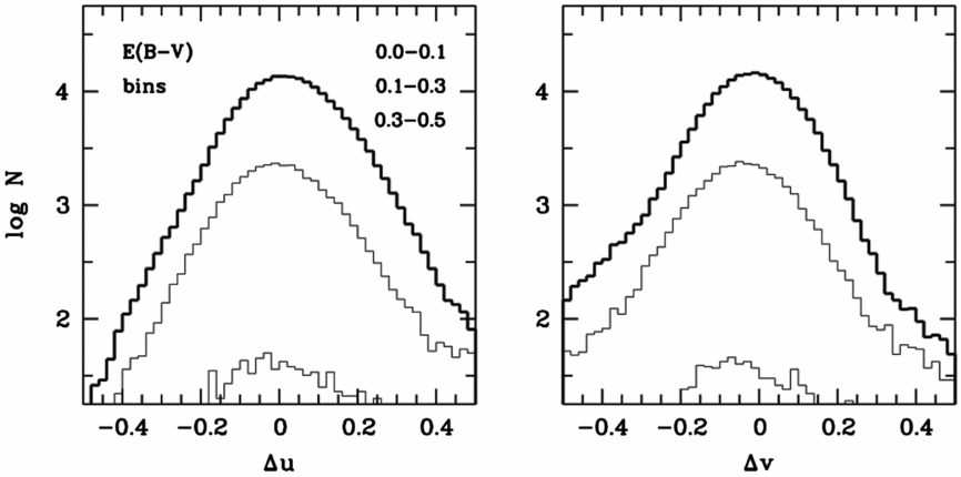
Figure 13. Difference between SkyMapper magnitudes and those predicted from PS1 photometry, as in Figure 12, but for the highly extrapolated filters u and v. The u-band has been globally adjusted by −0.05 mag, and the v-band shows a shift between regions of low vs. high reddening, which likely reflects the metallicity difference between the disk and halo populations in the Milky Way.
5.2. Morphology indicators
Separating point sources from extended sources is a challenge limited by the spatial resolution set by observing conditions and by PSF variations within a given frame. Any indicator of morphology will work best with bright sources but be increasingly ambiguous for noisier faint sources. We consider two morphology indicators: (i) the SExtractor stellarity index CLASS_STAR, which approaches 1.0 for point sources and typically has values between 0 and 0.9 for extended sources, and (ii) the difference between the PSF and Petrosian magnitudes.
In Figure 14, we show these two morphology indicators vs. the r-band magnitude for a large sample of objects including bright galaxies from the hemispheric 6dFGS and faint galaxies from the deeper and smaller area 2dFGRS (shown together with black points). We restrict the plotted sample to objects with good flags and no nearby neighbours. We note that both galaxy surveys contain compact galaxies, e.g., emission-line galaxies with high star-formation densities and active galaxies with dominant Seyfert-1 nuclei. In grey, we show a random sample of all DR1 objects matched in brightness to those two galaxy surveys. The two measures of morphology appear largely similar except for high-stellarity sources at the faint end: SExtractor tends not to attribute a high likelihood of stellarity to faint, noisy sources, while the difference between PSF and Petrosian magnitude for true point sources always scatters around zero, no matter the level of noise. Thus, CLASS_STAR tends to select proven point sources with low contamination and is incomplete at the faint end, while the magnitude comparison selects possible point sources with high completeness but increasing contamination at the faint end.
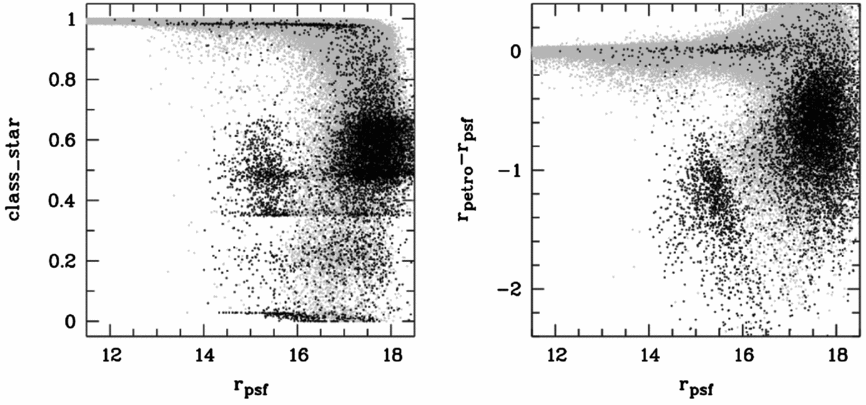
Figure 14. Morphology indicators vs. r-band magnitude: Left: SExtractor stellarity index CLASS_STAR. Right: Difference between PSF and Petrosian magnitude. Plotted are mag-limited galaxy samples from 6dFGS and 2dFGRS (black) and matching lower density samples of random DR1 objects (grey).
The fs_photometry table also contains for each separate detection our point-source likelihood measure CHI2_PSF, which is closer to the magnitude comparison in behaviour. It essentially expresses in χ2 units, how well the sequence of aperture magnitudes, i.e., growth curve, follows the local model of a PSF growth curve.
5.3. Survey depth and number counts
As DR1 includes only images from the Shallow Survey, it is expected to be ~4 mag shallower than the full SkyMapper survey. In Figure 15, we show number counts per filter from our master table. These typically turn over around 18 mag in each band, with the exception of the shallower, relatively narrow, v-band that appears complete to 17.5 mag. Galaxies are included in this plot although they will be incomplete already at much brighter magnitudes given that they are more extended than a PSF and their outer parts will get lost in the noise of the Shallow Survey images.
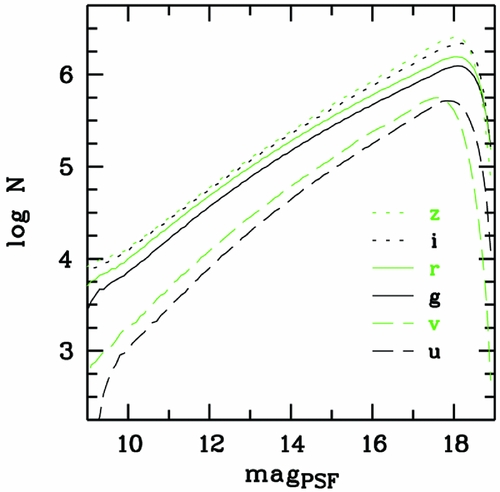
Figure 15. Number counts in PSF magnitude for each band. Except for the v-band, the completeness limit is nearly 18 mag.
A given mean population of stars can be roughly characterised by a horizontal line in Figure 15. The horizontal offset of the number count lines then shows the mean colours of the stellar population. This suggests, e.g., that a v-selected population with v < 17.5 will only be largely complete to z < 15.
5.4. Colour space and colour terms for stars
In Figure 16, we explore the locus of point sources in several dereddened colour–colour diagrams. We select stars from two magnitude bins (r = [12, 12.5] and r = [14, 14.5]) with low reddening E(B − V) < 0.1. The first two panels demonstrate how SkyMapper colours alone can differentiate between cool dwarfs and cool giants using the u − g colour, and between AF-type main-sequence stars and horizontal-branch (HB) stars using the u − v colour. The SkyMapper-specific u and v bands bracket the Hydrogen Balmer break at 365 nm, and lower surface gravity causes narrower Balmer absorption lines and thus higher v-band flux and a redder u − v colour.
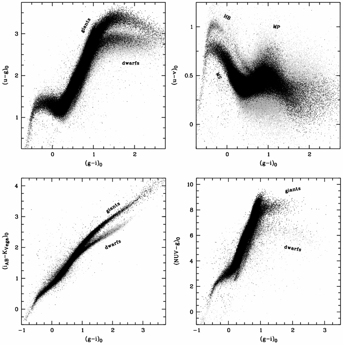
Figure 16. Dereddened SkyMapper colours measured for stars with E(B − V) < 0.1 and r PSF = [12, 12.5] (black) or r PSF = [14, 14.5] (grey). Top: Internal SkyMapper colours—we can easily see the bifurcation between cool dwarfs and cool giants in the top left panel, and separate horizontal branch (HB) stars from main-sequence (MS) stars in the top right panel; also shown is a region where metal-poor (MP) stars can be found easily. Bottom: Combined colour between a SkyMapper band and a 2MASS band or a GALEX band, respectively.
The bottom two panels exploit the fact that our database holds copies of the 2MASS and GALEX BCS catalogues (Bianchi, Conti, & Shiao Reference Bianchi, Conti and Shiao2014), to which we have pre-cross-matched all DR1 sources. Hence, multi-catalogue colours can be obtained with simple and fast table joins. In dereddening GALEX NUV magnitudes, we used R NUV = 7.04, which we derived by adding the empirical E(NUV − g) coefficient determined by Yuan, Liu, & Xiang (Reference Yuan, Liu and Xiang2013) to the R g of SDSS. The separation of the cool dwarf and giant branches is also clearly visible in optical-NIR colours such as i − K. Optical-to-near-UV colours such as NUV − g will further help to differentiate stars from galaxies and QSOs, when morphology or other indicators are unreliable.
Finally, in Figure 17, we show colour terms between the SkyMapper and SDSS bandpasses, from synthetic photometry performed on all Pickles stars (from main-sequence stars to supergiants) as well as on a grid of white dwarf spectra from Detlev Koester (private communication). We compare the SkyMapper u- and v-filters both to the SDSS u′-band, and the other four filters to their eponymous (g′r′i′z′) SDSS cousins. Between those cousins, the g-band shows the strongest colour terms, which reach up to 0.4 mag difference for cool stars.
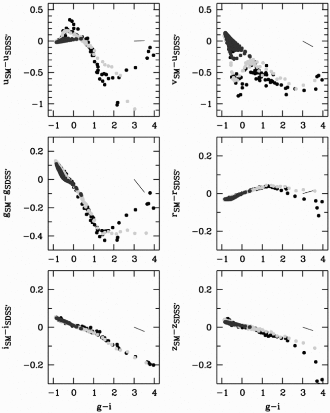
Figure 17. Colour terms between SkyMapper and SDSS for the spectral libraries of main-sequence (IV/V, black points) and giant (I–III, light grey points) F–M stars of Pickles (Reference Pickles1998), and a grid of DA/DB white dwarf spectra from T eff = [6000, 40000] K by Detlef Koester (priv. comm; dark grey points). The line shows a reddening vector for A V = 1 using a Fitzpatrick (Reference Fitzpatrick1999) law.
6 DATA ACCESS AND EXAMPLE APPLICATIONS
The DR1 dataset is available to the community through the SkyMapper NodeFootnote 15 of the All-Sky Virtual ObservatoryFootnote 16 (ASVO). The sky covered in the release can be browsed at the Node website, either in colour or in each individual SkyMapper passband, with the SkyViewer, a visual exploration tool based on Aladin Lite (Boch & Fernique Reference Boch and Fernique2014) and Hierarchical Progressive Survey methods (HiPS; Fernique et al Reference Fernique2015). The SkyMapper Node provides further tools that conform to the standards of the International Virtual Observatory AllianceFootnote 17 (IVOA), and includes catalogue access through the Table Access Protocol (TAP) and a Simple Cone Search function, as well as access to the reduced images (and their masks) through the Simple Image Access protocol (SIAP). Note that TAP queries are currently limited to returning one million rows at most.
The TAP tables are arranged in several distinct schemas, which group together the tables of each DR, plus the ‘ext’ schema of external catalogues. The layout of tables and the details of the SkyMapper table columns are provided in the Appendix. In the following, we discuss a few example applications together with the associated database TAP queries.
6.1. Properties of known variable stars
We investigated 256146 known variable stars from the AAVSO International Variable Star Index (VSX; Watson, Henden, & Price Reference Watson, Henden and Price2006, Reference Watson, Henden and Price2017) with cross-matches in DR1 and look for brightness variations seen by SkyMapper repeat visits. We obtain this information, e.g., for the r-band, from the database using the query:

Here, we avoid objects where the photometry may be affected by a range of effects captured in the FLAGS column, by bad pixels as captured in the NIMAFLAGS column, and by a merger of child objects (NCH_MAX).
In Figure 18, we show variability amplitudes vs. the known period or variability time scale of the stars, for all matches that have over 1 mag difference between the brightest and faintest good-quality detection in DR1. This information is of course available for all six SkyMapper bands, but we show only the v- and r-band to illustrate how the variability amplitude depends on the type of variable star and its temperature evolution.
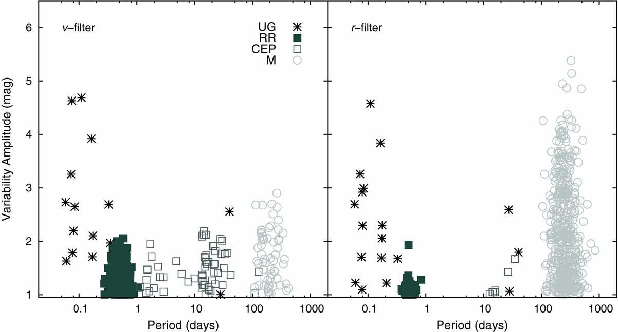
Figure 18. Variability amplitude of ~3 000 known variable stars from the AAVSO International Variable Star Index (VSX) with matches in DR1 and amplitudes in either v-band or r-band of over 1 mag. For clarity, this figure is restricted to U Geminorum stars (UG), RR Lyrae stars (RR), Cepheids (CEP), and Mira variables (M).
The combined high-amplitude list from these two bands contains 39 U Geminorum stars, 2,200 RR Lyrae stars, 55 Cepheids, and 520 Mira variables. Here, we omit further objects from rarer types and those with less characteristic time scales, such as eclipsing binaries. The variables thus end up clearly grouped by their types, which have characteristic and different time scales.
6.2. Long-term variability of QSOs
We investigated the variability of QSOs and Seyfert-1 galaxies identified by the Hamburg-ESO Survey (HES; Wisotzki et al. Reference Wisotzki, Christlieb, Bade, Beckmann, Köhler, Vanelle and Reimers2000). The public HES catalogue lists B J magnitudes measured on photographic plates exposed over 20 yr ago, which we compare to the SkyMapper g-band magnitudes observed in 2014/5 to study long-term variability. We can obtain a list of HES QSOs and their approximate magnitude change with a simple query.
However, with a more specific aim in mind, we look for candidates of low-redshift changing-look Seyfert galaxies; given that HES only includes broad-line AGN, this search is only sensitive to transitions from Sy-1 to Sy-2, which would manifest themselves by a large drop in brightness. We first restrict the list to redshifts below 0.3 and find 133 objects with a mean B J − g petro difference of +0.27 mag due to Vega-to-AB and bandpass differences, and an RMS scatter of 0.51 mag.
Taking the mean difference as indicating no variability, we search for objects with a brightness decline of more than 1 mag by selecting for B J − g petro − 0.27 < −1 using the query:
This query lists five candidates (see Table 3), which we have all followed-up spectroscopically with the ANU 2.3-m telescope and the WiFeS spectrograph (Dopita et al. Reference Dopita2010) in late 2017. All five Sy1-galaxies show a drop in UV continuum and the brightness of their broad Hydrogen emission lines, when compared to HES spectra taken two decades earlier. Three out of the five show little or no visible broad Hβ-emission any more, and thus have changed their type from Sy-1 to Sy-2.
Table 3. Candidates of low-redshift changing-look Seyfert galaxies identified by comparing SkyMapper DR1 g-band magnitudes with B J photometry reported by the Hamburg–ESO Survey (Wisotzki et al. Reference Wisotzki, Christlieb, Bade, Beckmann, Köhler, Vanelle and Reimers2000). Three out of five objects have changed from type-1 to (nearly) type-2 (quoted 2017 types are provisional).
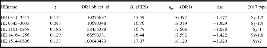
6.3. Selecting metal-poor star candidates
Identifying a large sample of chemically pristine stars in the Milky Way is a prime science driver for SkyMapper and a key motivation behind the distinct u- and v-filters (e.g., Keller et al. Reference Keller2007; Bessell et al. Reference Bessell, Bloxham, Schmidt, Keller, Tisserand and Francis2011). The v-filter, in particular, was designed to be metallicity-sensitive, especially at low metallicities where the greatly decreased significance of the Calcium H and K lines translates directly to enhanced flux. The release of SkyMapper DR1 facilitates a uniform search for EMP stars across the entire Southern hemisphere; the comparatively bright limit of the Shallow Survey is ideally suited to this task as high-resolution spectroscopic follow-up of stars fainter than magnitude ~16 is prohibitively expensive even on 8–10-m class facilities.
To identify EMP candidates we utilise a two-colour plot involving the g − i colour, which serves as a proxy for effective temperature and allows us to isolate stars of the desired spectral type, and the v − g colour, which indicates metallicity. On the plane defined by these two colours, stars with [Fe/H] < −2.5 are separated from the vast bulk of more metal-rich sources by more than ~0.5 mag; for giants with Teff ≈ 5000K, the spread between stars with [Fe/H] ≈ −2.5 and [Fe/H] ≈ −4.0 is ~0.1 mag. This selection strategy facilitated the discovery, from SkyMapper commissioning data, of the most iron-deficient star known (Keller et al. Reference Keller2014), which has [Fe/H] ⩽ −6.5 (Nordlander et al. Reference Nordlander2017). Our current DR1-based EMP survey is yielding stars at [Fe/H] ⩽ −3.0 with ~35% efficiency (see Da Costa et al. in preparation).
Before separating stars according to their colours, we select stellar objects with high-quality photometry from an area with reddening limited by E(B − V) < 0.2. We impose cuts on the g-band magnitude (<16), the photometric uncertainties in v, g, and i (0.05, 0.03, and 0.03 mag, respectively), the CLASS_STAR index (>0.9), the flags indicating any potential issues with the measurement (FLAGS <3 and NCH_MAX =1), and the location of the nearest neighbour (>7.5 arcsec), and we insist on at least one clean detection in all six filters and two in v (given its central importance). This translates into the query:
This defines a sample of 7.7 million sources, which cannot be downloaded in one step due to the current million-row limit for TAP queries. A subsequent colour analysis thins the list to ≈25000 high-quality candidates, those where the v − g colour suggests [Fe/H] ⩽ −2.5. Their spatial distribution is shown in the all-sky map of Figure 19 and exhibits the concentration towards the Galactic centre expected for a halo-like population, as well as some degree of sub-structure—although whether this is real or an artefact of residual imperfections in the photometric calibration is not yet understood (for example, note a deficiency in the number of candidates along a clear strip near α ≈ 280° and δ ≈ −65°).
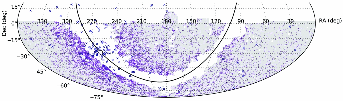
Figure 19. Map of EMP candidates with DR1 photometry suggesting [Fe/H] < −2.5: the shaded grey area marks the region from which candidates were selected after applying a selection for stars with high-quality photometry (see Section 6.3). The plane of the Milky Way is indicated with a solid line, and the Galactic centre with a large open circle. Known globular clusters are marked with blue crosses.
7 SURVEY FUTURE
Since 2015 March, observations with SkyMapper have focused on the deeper exposures for the Main Survey. Further visits of the Shallow Survey have continued during moon phases of >94%. The additional fourth and fifth passes of the Shallow Survey are dithered with much larger offsets than the first three visits; the first three are only intended to fill the gaps in the CCD mosaic, but the further visits involve approximate half-field dithers to assist with future plans to make the calibration more homogeneous. This can be implemented with an übercal approach, where measurements for common objects in overlapping parts of images help to constrain a fine tuning of all image ZPs (see also Padmanabhan et al. Reference Padmanabhan2008).
The Main Survey observes full colour sequences that are collected within 20 min, as well as additional gr image pairs added during dark time and iz image pairs primarily added during astronomical twilight. Since the Shallow Survey images are mostly limited by read-out noise, the Main Survey will be a full 4 mag deeper. We plan that, together, they will provide multiple independent and reliable measurements for over 99% of astronomical objects in the Southern sky at magnitudes ranging from 9 to 22. There will then also be more emphasis on extended-source and forced-position photometry.
However, the Shallow Survey presented in this paper will eventually serve as the calibration source for the Main Survey; it contains mostly point sources and many variable objects. Hence, this work has focused on instantaneous point-source photometry. The scientific analysis of DR1 has progressed over several topics, and spectroscopic follow-up of many sources has been started. This new dataset is already proving to be a treasure map for astronomers.
ACKNOWLEDGEMENTS
The national facility capability for SkyMapper has been funded through ARC LIEF grant LE130100104 from the Australian Research Council, awarded to the University of Sydney, the Australian National University, Swinburne University of Technology, the University of Queensland, the University of Western Australia, the University of Melbourne, Curtin University of Technology, and Monash University and the Australian Astronomical Observatory. SkyMapper is owned and operated by The Australian National University’s (ANU) Research School of Astronomy and Astrophysics (RSAA). The survey data were processed and provided by the SkyMapper Team at ANU. The SkyMapper node of the All-Sky Virtual Observatory is hosted at the National Computational Infrastructure (NCI). Parts of this project were conducted by the Australian Research Council Centre of Excellence for All-sky Astrophysics (CAASTRO), through project number CE110001020. BPS acknowledges support from the ARC Laureate Fellowship FL0992131. We acknowledge support from the ARC Discovery Projects DP0343962 (BPS, MSB), DP0878137 (BPS, MSB, GDC), DP120101237 (GDC, DM), and DP150103294 (GDC, DM). DM also acknowledges support from an ARC Future Fellowship FT160100206. This project was undertaken with the assistance of resources and services from the NCI, which is supported by the Australian Government.
This work has made use of data from the European Space Agency (ESA) mission Gaia,Footnote 18 processed by the Gaia Data Processing and Analysis ConsortiumFootnote 19 (DPAC). Funding for the DPAC has been provided by national institutions, in particular the institutions participating in the Gaia Multilateral Agreement. This paper makes use of data from the AAVSO Photometric All Sky Survey, whose funding has been provided by the Robert Martin Ayers Sciences Fund. We thank Sara Beck and Arne Henden from the American Association of Variable Star Observers for providing help with the APASS dataset. This publication makes use of data products from the Two Micron All Sky Survey, which is a joint project of the University of Massachusetts and the Infrared Processing and Analysis Center/California Institute of Technology, funded by the National Aeronautics and Space Administration and the National Science Foundation. We thank Bernie Shiao, Rick White, and Brian McLean from the Barbara A. Mikulski Archive for Space Telescopes (MAST) at the Space Telescope Science Institute for their help in obtaining the Pan-STARRS1 catalogues. The Pan-STARRS1 Surveys (PS1) and the PS1 public science archive have been made possible through contributions by the Institute for Astronomy, the University of Hawaii, the Pan-STARRS Project Office, the Max-Planck Society and its participating institutes, the Max Planck Institute for Astronomy, Heidelberg and the Max Planck Institute for Extraterrestrial Physics, Garching, The Johns Hopkins University, Durham University, the University of Edinburgh, the Queen’s University Belfast, the Harvard-Smithsonian Center for Astrophysics, the Las Cumbres Observatory Global Telescope Network Incorporated, the National Central University of Taiwan, the Space Telescope Science Institute, the National Aeronautics and Space Administration under Grant No. NNX08AR22G issued through the Planetary Science Division of the NASA Science Mission Directorate, the National Science Foundation Grant No. AST-1238877, the University of Maryland, Eotvos Lorand University (ELTE), the Los Alamos National Laboratory, and the Gordon and Betty Moore Foundation. We thank Michal Kočer, then of the Kleť Observatory in the Czech Republic, for sharing copies of the UCAC4 astrometry index files. We thank the IT and technical staff at RSAA Mt Stromlo, in particular Gabe Bloxham, Joshua Rich, Bill Roberts, Kim Sebo, Annino Vaccarella, and Col Vest, as well as Ian Adams and Peter Verwayen at Siding Spring Observatory, for persistent support on hardware, software, and the telescope. We thank the staff at CDS, Strasbourg Observatory, France, for crucial support in creating the SkyMapper SkyViewer. This research made use of Astropy, a community-developed core Python package for Astronomy (Astropy Collaboration 2013). We thank Roger Smith at Caltech and Mark Downing at ESO for suggestions related to the detector ‘tearing’. We thank Lutz Wisotzki from AIP Potsdam for providing us with spectra from the Hamburg-ESO Survey. We also thank Helmut Jerjen, Anais Möller, and the anonymous referee for a very careful reading and comments improving the manuscript. We acknowledge the Gamilaroi people as the traditional owners of the land on which the SkyMapper Telescope stands.
A SOURCE EXTRACTOR PARAMETERS AND TAP TABLE SCHEMA
In Table A1, we list the SExtractor parameters that are used and recorded in the DR1 photometry tables.
Table A1. Source extractor parameters measured.
In Table A2, we show the structure of tables in the various schemas of the SkyMapper ASVO TAP service. Each SkyMapper DR has its own schema, and external catalogues are collected into the ‘ext’ schema. Tables A3–A7 provide descriptions of each column within the SkyMapper ASVO tables.
Table A2. Schemas and tables contained in the SkyMapper ASVO TAP service.
Table A3. DR1 master table database schema.
Table A4. DR1 fs_photometry table database schema.
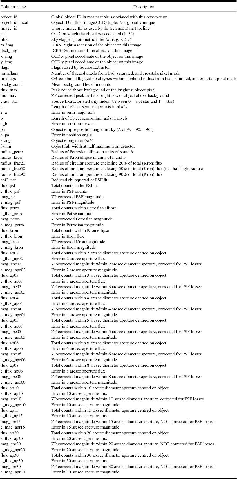
Table A5. DR1 ccds table database schema.
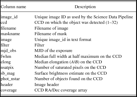
Table A6. DR1 images table database schema.
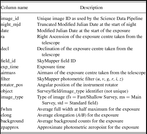
Table A7. DR1 mosaic table database schema.