1 INTRODUCTION
Galaxies are complex structures assembled through a variety of physical processes which act at different stages of their life, such as gas accretion; star formation; disc formation, growth, and buckling; bar formation and buckling etc.; as well as mergers and interactions with neighbouring galaxies. The result is a rich variety of galactic components in the observed galaxy population. Classifying galaxies based on these structures, in the optical and/or near-infrared bands has been and still is now common practise (e.g., Jeans Reference Jeans1919, Hubble Reference Hubble1926, de Vaucouleurs Reference de Vaucouleurs1959, Sandage Reference Sandage, Sandage, Sandage and Kristian1975, de Vaucouleurs et al. Reference de Vaucouleurs, de Vaucouleurs, Corwin, Buta, Paturel and Fouqué1991, Abraham, van den Bergh, & Nair Reference Abraham, van den Bergh and Nair2003, Buta et al. Reference Buta2015, etc.).
A quantitative structural classification requires a reliable method to separate out each structural component from the others that make up the galaxy. Moreover, individually analysing each constituent probes, the specific physical or dynamical processes associated with it and thus provides insight into galaxy evolution. The common practise is to model one of the fundamental diagnostics of a galaxy’s structure, namely its radial light (or surface brightness) profile (SBP), by decomposing it into a sum of analytical functions, with each function representing a single component (e.g., Prieto et al. Reference Prieto, Aguerri, Varela and Muñoz-Tuñón2001, Balcells et al. Reference Balcells, Graham, Domínguez-Palmero and Peletier2003, Blanton et al. Reference Blanton2003, Naab & Trujillo Reference Naab and Trujillo2006, Graham & Worley Reference Graham and Worley2008). See Graham Reference Graham, Oswalt and Keel2013 for a comprehensive review of modelling the light profile of galaxies.
One of the best methods to extract an SBP from a galaxy image is by fitting quasi-elliptical isophotes as a function of increasing distance from the photometric centre of the galaxy. In such schemes, the isophotes are free to change their axis ratio, or ellipticity, position angle (PA), and shape (quantified through Fourier harmonics) with radius, which ensures that the models capture the galaxy light very well. A popular tool for this is the IRAF task Ellipse (Jedrzejewski Reference Jedrzejewski1987), which works well for galaxies whose isophotes display low-level deviations from pure ellipses, such as elliptical galaxies or disc galaxies viewed relatively face-on. For more complex isophotal structures however, such as edge-on disc galaxies, X/peanut-shaped bulges, bars, and barlenses, Ellipse has been shown to fail and the newer IRAF task Isofit Footnote 1 (Ciambur Reference Ciambur2015) is more appropriate.
A somewhat different approach in performing galaxy decomposition is to directly fit the galaxy’s projected light distribution, i.e. the galaxy image, in two dimensions (2D). Recent years have seen the advent and development of a number of programs dedicated to this purpose, notably GIM2D (Simard et al. Reference Simard2002), Budda (de Souza, Gadotti, & dos Anjos Reference de Souza, Gadotti and dos Anjos2004), Galfit (Peng et al. Reference Peng, Ho, Impey and Rix2010), and Imfit (Erwin Reference Erwin2015).
In support for the 2D method, Erwin (Reference Erwin2015) has invoked several drawbacks of one-dimensional (1D) profile modelling, namely that it is unclear which azimuthal direction to model (major axis, minor axis, or other), that most of the data from the image is discarded, and that non-axisymmetric components (such as bars) can be misinterpreted as axisymmetric components, and their properties cannot be extracted from a 1D light profile. While these issues certainly apply when one extracts the SBP by taking a 1D cut from a galaxy image, all of these issues are resolved if the SBP is obtained from an isophotal analysis. In particular, fitting isophotes makes use of the entire image (so no data is discarded) and apart from the SBP itself, this process additionally provides information about the isophotes’ ellipticities, PAs, and deviations from ellipticity (in the form of Fourier modes). All of this information is sufficient to completely reconstruct the galaxy image for even highly complex and non-axisymmetric isophote shapes (see Ciambur Reference Ciambur2015 and Section 5 of this paper). Having these extra isophote parameters allows one to obtain the SBP along any azimuthal direction, and identify and quantitatively study non-axisymmetric components such as bars or even peanut/X-shaped bulges (Ciambur & Graham Reference Ciambur and Graham2016). It is therefore recommended to always use isophote tables rather than image cuts in 1D decompositions.
Overall, both 1D and 2D decomposition techniques present benefits as well as disadvantages. The 2D image-modelling technique has the advantage that every pixel (except those deliberately masked out due to contaminating sources) in the image contributes directly to the fitting process, whereas in an isophotal (1D) analysis, pixels contribute in an azimuthal-average sense. Multicomponent systems with different photometric centres can also pose a problem for 1D SBPs, which assume a single centre for all components at R = 0Footnote 2 , but can however be easily modelled in 2D. On the other hand, 2D codes suffer from the fact that each component has a single, fixed value for the ellipticity, PA, and Fourier moments (such as boxyness or discyness, and also higher orders), which can in some cases limit the method considerably. Triaxial ellipsoids viewed in projection can have radial gradients in their ellipticities and PAs (Binney Reference Binney1978, Mihalas & Binney Reference Mihalas and Binney1981), an effect captured in a 1D isophotal analysis (where both quantities can change with radius) but not in a 2D decompositionFootnote 3 .
There are notable examples in the literature where the 1D method has been preferred over the 2D technique. One such case is the decomposition of the Atlas 3D (Cappellari et al. Reference Cappellari2011) sampleFootnote 4 of early-type galaxies, in Krajnović et al. (Reference Krajnović2013). I point the reader to Section 2 and Appendix A of their paper, where they discuss both methods and test the performance of their preferred 1D method against a 2D analysis (with Galfit). Another illuminating example is in Savorgnan & Graham (Reference Savorgnan and Graham2016). They performed both 1D (with private code) and 2D (with Imfit) decompositions of 72 galaxies, out of which 41 did not converge or did not give meaningful solutions in 2D, whereas only nine could not be modelled in 1D. Section 4.1 in their paper also provides an insightful and practical comparison between 1D and 2D galaxy modelling techniques.
The past few decades have seen a flurry of 2D image-fitting codes, whereas publicly available tools that focus on 1D decompositions are scarce. In this paper, I present Profiler, a freely available code written in Python, designed to provide a fast, flexible, user-friendly, and accurate platform for performing structural decompositions of galaxy SBP.
The remainder of the paper is structured as follows. In Section 2, I describe the input data and information required by Profiler prior to the decomposition process. Section 3 is a concise review of typical galaxy components and the analytical functions employed to model them. Section 4 then details the fitting process, and Section 5 provides three example applications, each illustrating different features of Profiler. Finally, I summarise and conclude with Section 6.
2 THE INPUT DATA
With a view to streamline the decomposition process, Profiler has a built-in Graphical User Interface (GUI) coded in the standard Python package TkInter. This ensures that the decomposition process is entirely interactive, with all settings, options, and input information readily changeable through buttons, text-box, and check-box widgets in the main GUI. Thus, the need to perpetually change a separate configuration file each time one wishes to modify settings is eliminated, and the user can employ the visualisation tools (which will be discussed in Section 5) and the GUI to make any required tweaks, until the solution is reached. Figure 1 presents the GUI, with most widgets active for illustration purposes. Note that the user must specify all this galaxy-specific information on a case-by-case basis, as is detailed below.
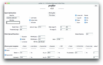
Figure 1. The Profiler GUI, with two active components (Sérsic and exponential) for illustration purposes. All the text-boxes and check-boxes are set to default values, and must be changed by the user to the specifics of the data (see text for details). The component parameters too must be set to initial guess-values, from which the code obtains the best-fitting solution.
2.1. The surface brightness profile
Profiler was designed to work with isophote tables generated by either Ellipse or Isofit. Apart from the galaxy light profile itself, the two programs provide useful ancillary information such as the isophotes’ ellipticities, PAs, departures from pure ellipses, etc. Alternatively, the user can provide a simple table consisting of two columns, namely radius R and intensity I(R).
Instrument-specific details are additionally required, in particular the CCD angular size of a pixel, in arcsec, and the zero-point magnitude. The isophote intensity I is then converted into surface brightness μ (in magnitudes arcsec−2) through
 $$\begin{equation}
\mu (R) = m_0 - 2.5{\rm log}_{10}\left[\frac{I(R)}{ps^2}\right],
\end{equation}$$
$$\begin{equation}
\mu (R) = m_0 - 2.5{\rm log}_{10}\left[\frac{I(R)}{ps^2}\right],
\end{equation}$$
where m 0 is the zero-point magnitude and ps is the pixel angular size. In Equation (1), R generally corresponds to the isophote’s semi-major axis (R maj). Often the major axis profile is mapped onto the ‘equivalent’, or geometric mean axis, R eq, through
 $$\begin{equation}
R_{\rm eq} = R_{\rm maj}\sqrt{1 - \epsilon (R_{\rm maj})},
\end{equation}$$
$$\begin{equation}
R_{\rm eq} = R_{\rm maj}\sqrt{1 - \epsilon (R_{\rm maj})},
\end{equation}$$
where ε(R maj) is the isophote ellipticity, defined as 1 minus the axis ratio. This mapping converts the isophote into the equivalent circle that conserves the original surface area of the isophote (see the Appendix of Ciambur Reference Ciambur2015 for a derivation). The equivalent axis profile is thus circularly symmetric, and decomposing it allows for an analytical computation of the total magnitude of components directly from their parameters (e.g., Graham & Driver Reference Graham and Driver2005 for Sérsic parameters).
The user has a choice between modelling the profile along R maj (the default) or R eq. For the latter option, provided that the input data contains ellipticity information, Profiler generates the equivalent axis profile internally and outputs the total magnitudes of components after the decomposition. If the input data is a two-column table, it is assumed that the R column is already the axis chosen by the user. Whenever the sampling step ΔR between successive isophotes is not constant, Profiler linearly interpolates the SBP internally on a uniformly spaced radial axis before performing the PSF convolution.
2.2. The point spread function
The ability of telescopes to resolve a point-source is dictated by a number of factors, including their diffraction limit (due to the fact that they have a finite aperture), the detector spatial resolution (pixel size) and, for ground-based instruments, the distortion of wavefronts caused by turbulent mixing in the atmosphere, an effect known as ‘seeing’. All of these effects blur astronomical images, spreading the light at every point in a way characteristic to each instrument. In an ideal image, a point source’s profile is a delta function. In a real image, however, the functional form is called the instrumental point spread function (PSF). In order to reconstruct the true distribution of light in an image, it is essential to know the PSF at every point across the focal plane.
The most basic aproximation of a PSF is a Gaussian functional form with the single parameter FWHM (or dispersion σ, the two being related by FWHM = $2\sigma \sqrt{2\,{\rm ln}2}$
). This form, however, underestimates the flux in the ‘wings’ of the PSF, which can bias decomposition parameters (Trujillo et al. Reference Trujillo, Aguerri, Cepa and Gutiérrez2001b found the effect to range between 10–30% for Sérsic parameters).
$2\sigma \sqrt{2\,{\rm ln}2}$
). This form, however, underestimates the flux in the ‘wings’ of the PSF, which can bias decomposition parameters (Trujillo et al. Reference Trujillo, Aguerri, Cepa and Gutiérrez2001b found the effect to range between 10–30% for Sérsic parameters).
A more realistic approximation which is capable of modelling PSF wings is the Moffat profile (Moffat Reference Moffat1969), given by
 $$\begin{equation}
I(R) = I_0 \,\left[1+\left( \frac{R}{\alpha }\right)^2\right]^{-\beta },
\end{equation}$$
$$\begin{equation}
I(R) = I_0 \,\left[1+\left( \frac{R}{\alpha }\right)^2\right]^{-\beta },
\end{equation}$$
where α is a characteristic width related to the FWHM by the identity FWHM = $2\alpha \sqrt{2^{1/\beta }-1}$
, and β controls the amount of light in the ‘wings’ of the profile compared to the centre (redistributing the light of the central peak into wings mimics the effect of spreading light in Airy rings). Figure 2 shows Moffat functions of the same FWHM but different values of β, as well as the limiting case where β → ∞, which corresponds to a Gaussian (Trujillo et al. Reference Trujillo, Aguerri, Cepa and Gutiérrez2001b).
$2\alpha \sqrt{2^{1/\beta }-1}$
, and β controls the amount of light in the ‘wings’ of the profile compared to the centre (redistributing the light of the central peak into wings mimics the effect of spreading light in Airy rings). Figure 2 shows Moffat functions of the same FWHM but different values of β, as well as the limiting case where β → ∞, which corresponds to a Gaussian (Trujillo et al. Reference Trujillo, Aguerri, Cepa and Gutiérrez2001b).

Figure 2. Different point spread functions represented as intensity vs. radius, in arbitrary units. The Moffat function (black curves) accounts for seeing effects (e.g., Airy rings) by transferring flux from the peak of the PSF into its wings. This is controlled by the β parameter and, for large values of β the Moffat approaches a Gaussian (red curve). All curves plotted here have an FWHM of 0.5.
In practise, when characterising the PSF the usual norm is to fit either a Gaussian or a Moffat profile on bright, unsaturated stars in the image with e.g., the IRAF task Imexamine. This task directly provides the FWHM for the former and (FWHM; β) for the latter case.
In Profiler, the user has a choice of either Gaussian, Moffat, or data vector PSF. The first two require the parameters specific to each function, from which Profilergenerates the PSF internally when needed. The third option requires a table of values, R and I(R), in the form of a text file provided by the userFootnote 5 . The radial extent of the data vector PSF is required by Profiler to at least match or exceed that of the galaxy profile. As I will show in Section 5.3, this feature is very useful when the analytical functions above do not provide a sufficiently exact description of the PSF.
3 THE MODEL
Profiler can employ several analytical functions to model the radial light profiles of a galaxy’s constituent components. The user is free to add an indefinite number of components to the model, and each component (function) can have its parameters freely varying or fixed to given values during the fit.
In the remainder, I provide a description of each function available in Profiler in the context of the photometric component(s) which it is intended to model. A summary of all the functions, with their typical uses and number of parameters, is provided in Table 1 at the end of this section.
Table 1. An index of the functions available in Profiler.
3.1. Ellipticals and galaxy bulges
3.1.1. The Sérsic model
There have been many attempts in the past to analytically describe the SBPs of elliptical galaxies, including deVaucouleurs’ R 1/4 ‘law’ (de Vaucouleurs Reference de Vaucouleurs1948, Reference de Vaucouleurs1953), the King profile (King Reference King1962, Reference King1966), etc. See Graham (Reference Graham, Oswalt and Keel2013) for a review of these past efforts. At present, it is generally agreed that the most robust function for this purpose is given by the Sérsic (Reference Sérsic1963) R 1/n model (Caon, Capaccioli, & D’Onofrio Reference Caon, Capaccioli and D’Onofrio1993, D’Onofrio, Capaccioli, & Caon Reference D’Onofrio, Capaccioli and Caon1994).
While the Sérsic function in itself does not contain any physical meaning, it is remarkably flexible and can accurately capture the light profiles of a broad range of spheroid components, from the small bulges of late-type spiral galaxies to the highly concentrated light profiles of bright elliptical galaxies. Additionally (as will be discussed in the following sections), the Sérsic profile can model discs and bars.
The Sérsic profile is parameterised by three quantities: the radius enclosing half of the light, Re , the intensity at this radius, Ie = I(Re ), and the concentration, or Sérsic index, n. It takes the form
 $$\begin{equation}
I(R) = I_e {\rm exp} \left\lbrace -b_n \left[ \left( \frac{R}{R_e} \right)^{\frac{1}{n}} -1 \right] \right\rbrace ,
\end{equation}$$
$$\begin{equation}
I(R) = I_e {\rm exp} \left\lbrace -b_n \left[ \left( \frac{R}{R_e} \right)^{\frac{1}{n}} -1 \right] \right\rbrace ,
\end{equation}$$
where bn depends on n and is obtained by solving
 $$\begin{equation}
\Gamma (2n) = 2\gamma (2n, b_n),
\end{equation}$$
$$\begin{equation}
\Gamma (2n) = 2\gamma (2n, b_n),
\end{equation}$$
where Γ is the (complete) gamma function and γ the incomplete gamma function, given by the integral
 $$\begin{equation}
\gamma (2n,x) = \int _0^{x} {\rm e}^{-t} t^{2n -1} {\rm d}t.
\end{equation}$$
$$\begin{equation}
\gamma (2n,x) = \int _0^{x} {\rm e}^{-t} t^{2n -1} {\rm d}t.
\end{equation}$$
Figure 3 shows the Sérsic profile for a range of concentration parameters (n). The reader will also find a review of the Sérsic model, useful equations pertaining to it, as well as early references, in Graham & Driver (Reference Graham and Driver2005).
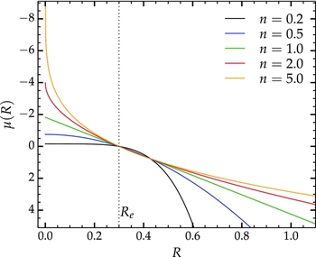
Figure 3. The Sérsic profile for five values of the Sérsic index n. The curves represent surface brightness as a function of radius, in arbitrary units, and all profiles have the same values of μe and R e. The half-light radius, R e, is indicated by the vertical dotted line.
3.1.2. The core-Sérsic model
The most luminous early-type galaxies display ‘cored’ central profiles, thought to be the result of black hole binary systems kicking out stars through 3-body interactions (Begelman, Blandford, & Rees Reference Begelman, Blandford and Rees1980), thus causing a deficit of light in the centre (King Reference King1978, Dullo & Graham Reference Dullo and Graham2012, Reference Dullo and Graham2014 and references therein). An ideal functional form which describes these types of objects is the 6-parameter core-Sérsic model (Graham et al. Reference Graham, Erwin, Trujillo and Asensio Ramos2003), given by
 $$\begin{equation}
I(R) = I^{\prime } \left[ 1 + \left( \frac{R_b}{R} \right)^{\alpha } \right]^{\frac{\gamma }{\alpha }} {\rm exp} \left\lbrace -b_n \left[ \frac{R^{\alpha } + R_b^{\alpha }}{R_e^{\alpha }} \right]^{\frac{1}{\alpha n}} \right\rbrace .
\end{equation}$$
$$\begin{equation}
I(R) = I^{\prime } \left[ 1 + \left( \frac{R_b}{R} \right)^{\alpha } \right]^{\frac{\gamma }{\alpha }} {\rm exp} \left\lbrace -b_n \left[ \frac{R^{\alpha } + R_b^{\alpha }}{R_e^{\alpha }} \right]^{\frac{1}{\alpha n}} \right\rbrace .
\end{equation}$$
The core-Sérsic function takes the form of a power law in the core region, which then transitions into a Sérsic form outside the core region (Figure 4). It is parameterised by the break (transition) radius Rb and half-light radius Re , the inner profile slope γ, the smoothness of the transition, controlled by α, the Sérsic index n and a normalisation, or scale intensity I′, which is related to the intensity at the break radius through Equation (6) in Graham et al. (Reference Graham, Erwin, Trujillo and Asensio Ramos2003), that is
 $$\begin{equation}
I^{\prime } = I_b\;2^{-\gamma /\alpha }\;{\rm exp} \left[ b_n \left( \frac{2^{1/\alpha } R_b}{R_e} \right)^{1/n} \right].
\end{equation}$$
$$\begin{equation}
I^{\prime } = I_b\;2^{-\gamma /\alpha }\;{\rm exp} \left[ b_n \left( \frac{2^{1/\alpha } R_b}{R_e} \right)^{1/n} \right].
\end{equation}$$
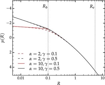
Figure 4. The core-Sérsic profile. The curves represent surface brightness as a function of radius, in arbitrary units. Red curves illustrate the effect of varying the inner slope γ, while black curves illustrate changing the break sharpness α. The break radius and effective radius are indicated through the vertical dotted lines, and are marked as Rb and Re , respectively.
The core-Sérsic model has also been recently implemented in 2D fitting codes, specifically in the Galfit add-on code Galfit-Corsair (Bonfini Reference Bonfini2014), and in Imfit (Erwin Reference Erwin2015).
3.2. Discs
3.2.1. The exponential model
The radial decline of light in flat galaxy discs has long been known to be approximately exponential (Patterson Reference Patterson1940, de Vaucouleurs Reference de Vaucouleurs1957, Freeman Reference Freeman1970). For disc components, Profiler can employ the two-parameter exponential model:
 $$\begin{equation}
I(R) = I_0\, {\rm exp}\left(-\frac{R}{h}\right),
\end{equation}$$
$$\begin{equation}
I(R) = I_0\, {\rm exp}\left(-\frac{R}{h}\right),
\end{equation}$$
where I 0 is the intensity at R = 0 and h is the exponential scale length, which corresponds to the length in which the light diminishes by a factor of e, i.e., I(h) = I 0/e.
3.2.2. The broken exponential model
While the light profiles of galaxy discs are commonly assumed to be characterised by a single exponential for their whole extent (galaxies for which this is true are said to have ‘Type I’ profiles in the classification of Erwin, Pohlen, & Beckman Reference Erwin, Pohlen and Beckman2008), as many as 90% (Pohlen & Trujillo Reference Pohlen and Trujillo2006) of disc galaxies display a ‘break’ in their light profiles, typically at a few scale lengths from the photocentre (van der Kruit Reference van der Kruit1987, Pohlen et al. Reference Pohlen, Beckman, Hüttemeister, Knapen, Erwin, Dettmar, Block, Puerari, Freeman, Groess and Block2004). More specifically, this is an abrupt change in their exponential scale length (Figure 5). This phenomenon is referred to as a truncation, or ‘Type II’ profile, if the scale length decreases (the light fall-off becomes steeper) and an anti-truncation, or ‘Type III’ profile (Erwin, Beckman, & Pohlen Reference Erwin, Beckman and Pohlen2005), if the scale-length becomes longer (the fall-off becomes shallower). Profiler provides a broken exponential function to fit these types of profiles [Equation (10)], characterised by four free parameters: The central flux I 0, the break radius Rb , and the inner and outer scale lengths, h 1 and h 2, respectively.
 $$\begin{equation}
I(R) = \left\lbrace \begin{array}{@{}l@{\quad }l@{}}I_0\, {\rm exp} \left(-R/h_1\right), & R \leqslant R_{b}\\
I_{b}\, {\rm exp} \left[-(R-R_{b})/h_2\right], & R > R_{b} \:, \end{array}\right.
\end{equation}$$
$$\begin{equation}
I(R) = \left\lbrace \begin{array}{@{}l@{\quad }l@{}}I_0\, {\rm exp} \left(-R/h_1\right), & R \leqslant R_{b}\\
I_{b}\, {\rm exp} \left[-(R-R_{b})/h_2\right], & R > R_{b} \:, \end{array}\right.
\end{equation}$$
where Ib is the brightness at the break radius, and is not a free parameter since Ib = I(Rb ).
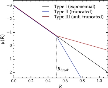
Figure 5. The three types of exponential disc models represented as surface brightness vs. radius, in arbitrary units. The black curve is a single exponential (Type I) profile. The broken exponential profile takes two forms: the Type II, or truncated, profile (h2 < h1, blue), and the Type III, or anti-truncated profile (h2 > h1, red).
3.2.3. The Edge-on disc model
When disc galaxies are viewed in close to edge-on orientation, the disc SBP exhibits a gradually shallower slope towards the centre (van der Kruit & Searle Reference van der Kruit and Searle1981; Pastrav et al. Reference Pastrav, Popescu, Tuffs and Sansom2013). In this regime, Profiler can use two special cases of the inclined disc profile of van der Kruit & Searle (Reference van der Kruit and Searle1981), which is defined in 2D as a function of major axis R and minor axis Z, as
 $$\begin{equation}
I(R,Z) = I_0\, \left( \frac{R}{h_r} \right) \,K_1\left( \frac{R}{h_r} \right)\, {\rm sech}^2\left( \frac{Z}{h_{z}} \right) ,
\end{equation}$$
$$\begin{equation}
I(R,Z) = I_0\, \left( \frac{R}{h_r} \right) \,K_1\left( \frac{R}{h_r} \right)\, {\rm sech}^2\left( \frac{Z}{h_{z}} \right) ,
\end{equation}$$
where I 0 is the central intensity, hr is the scale length in the plane of the disc (major axis), hz is the scale length in the vertical (minor axis) direction (⊥ to the disc plane), and K 1 is the modified Bessel function of the second kind.
In the limiting case of Z = 0, Equation (11) reduces to the major axis form
 $$\begin{equation}
I(R_{\rm maj}) = I_0\, \left( \frac{R_{\rm maj}}{h_r} \right) \,K_1\left( \frac{R_{\rm maj}}{h_r} \right).
\end{equation}$$
$$\begin{equation}
I(R_{\rm maj}) = I_0\, \left( \frac{R_{\rm maj}}{h_r} \right) \,K_1\left( \frac{R_{\rm maj}}{h_r} \right).
\end{equation}$$
Similarly, along the minor axis (R = 0), Equation (11) reduces to
 $$\begin{equation}
I(R_{\rm min}) = I_0\, {\rm sech}^2\left( \frac{R_{\rm min}}{h_z} \right).
\end{equation}$$
$$\begin{equation}
I(R_{\rm min}) = I_0\, {\rm sech}^2\left( \frac{R_{\rm min}}{h_z} \right).
\end{equation}$$
Profiler can employ Equations (12) and (13) to fit edge-on discs along the major and minor axes, respectively. Note that neither hr nor hz are equal to the exponential scale length h. Their corresponding profiles do not decrease in intensity by a factor of e at every hr or hz (see van der Kruit & Searle Reference van der Kruit and Searle1981 for more details on the definition of these two scale parameters). One can readily discern this visually in Figure 6 ( blue and green curves): The curvature of these profiles towards R → 0 implies that they cannot be characterised by a single value for the e-folding radius, as exponential profiles are. Rather, the e-folding starts off large towards the centre (where the slopes are shallower) and gradually decreases with increasing R. At high radii, the e-foldings asymptote to constant values and therefore both profiles approach exponential forms. The major-axis profile has an e-folding length (from R = 0) equal to 1.658hr , whereas the minor-axis profile has an e-folding length equal to 1.085hz Footnote 6 . This is illustrated in Figure 6.

Figure 6. Various disc models: exponential (black, solid), edge-on disc along major-axis [Equation (12); blue, solid], edge-on disc along the minor-axis (Equation (13); green, solid), and Sérsic (n = 0.7; red, dashed). The profiles are represented as surface brightness vs. radius, in arbitrary units. They all have the same central surface brightness (μ0) and the same e-folding radius, equal to h, the exponential scale length. The vertical dotted lines mark each profile’s characteristic scale length (keeping the colour scheme).
3.2.4. The Sérsic model for discs
The Sérsic function can also successfully model discs. The n = 1 Sérsic function is identical to an exponential and can be used to model Type I profiles, while inclined (edge-on) discs, or those with dusty centres, may be fitted with n < 1 Sérsic functions (typically in the range n ~ 0.7-0.9; see Figure 6). In this case, one can still recover its e-folding length hS and central surface brightness μ0 from
 $$\begin{equation}
h_S = \frac{R_e}{(b_n)^n} ,
\end{equation}$$
$$\begin{equation}
h_S = \frac{R_e}{(b_n)^n} ,
\end{equation}$$
and
 $$\begin{equation}
\mu _0 = \mu _e - \frac{2.5}{{\rm ln}(10)}b_n .
\end{equation}$$
$$\begin{equation}
\mu _0 = \mu _e - \frac{2.5}{{\rm ln}(10)}b_n .
\end{equation}$$
As before, if n ≠ 1, the e-folding radius is not unique along the whole profile and is again highest towards the centre and lower at high-R. When n = 1, Equations (14) and (15) reduce to hS = Re /1.67835 and μ0 = μ e − 1.82224, respectively. Unlike the edge-on disc model, the n < 1 Sérsic function does not asymptote to an exponential, but has an ever steeper slope with increasing R (see Figure 3).
3.3. Bars
Bars are common in disc galaxies (the fraction is ~ 2/3 in the near-infrared; Eskridge et al. Reference Eskridge2000, Menéndez-Delmestre et al. Reference Menéndez-Delmestre, Sheth, Schinnerer, Jarrett and Scoville2007, Laurikainen et al. Reference Laurikainen, Salo, Buta and Knapen2009, Nair & Abraham Reference Nair and Abraham2010) and display a characteristic flat profile which ends with a relatively sharp drop-off. This shows up in SBPs as a ‘shelf’-like or ‘shoulder’-like feature, usually (but not necessarily) between the inner spheroid component and the outer disc. Bars are often modelled with the four-parameter Ferrers profile (Ferrers Reference Ferrers1877), expressed as
 $$\begin{equation}
I(R) = I_0\, \left[ 1- \left(\frac{R}{R_{\rm end}} \right)^{2-\beta } \right]^{\alpha },
\end{equation}$$
$$\begin{equation}
I(R) = I_0\, \left[ 1- \left(\frac{R}{R_{\rm end}} \right)^{2-\beta } \right]^{\alpha },
\end{equation}$$
where I 0 is the central brightness, R end is the cut-off radius, and α and β control the inner slope and break sharpness (see Figure 7). Note that β > 0 causes a cusp in the central parts of the profile. As there is no observational evidence that the profiles of bars display such a cusp, it is recommended that β be set to 0.

Figure 7. Possible bar components: the black and blue curves are all Ferrers profiles [Equation (16)] with the same central surface brightness (μ0) and end radius (R end), but different permutations of the α and β parameters, such that curves of the same colour illustrate the effect of changing β, while curves of the same style (i.e., solid vs. dashed) illustrate the effect of changing α. All profiles are represented as surface brightness vs. radius, in arbitrary units.
Another function which can be used to model bars is a low-n Sérsic function (typically in the range n ≲ 0.1–0.5, the drop-off being sharper the lower n is; see Figure 7, red curve).
3.4. Rings and spiral arms
The presence of spiral arms in a disc can cause deviations from an exponential profile in the form of ‘bumps’ (Erwin et al. Reference Erwin, Beckman and Pohlen2005). A stellar ring also causes a ‘bump’ in the profile. These features are modelled in Profiler via the three-component Gaussian profile, given by
 $$\begin{equation}
I(R) = I(R_r) \, {\rm exp}\left[ -\frac{(R-R_r)^2}{2\sigma ^2}\right],
\end{equation}$$
$$\begin{equation}
I(R) = I(R_r) \, {\rm exp}\left[ -\frac{(R-R_r)^2}{2\sigma ^2}\right],
\end{equation}$$
where Rr is the radius of the bump, I(Rr ) is its peak intensity, and σ its width (dispersion).
4 FITTING THE DATA
Once the required input information is provided, the user must make a choice of components that are to make up the model. Before this (or at any point after having provided the input information), they can visualise the galaxy light profile and, if it is based on isophote fits with Ellipse or Isofit, the ellipticity ε, PA or B 4 (fourth cosine harmonic amplitude) profiles can be displayed. This helps the user decide which components to use and make an educated guess for the initial values of their parameters. The default setting is that all model parameters are free, but the user has a choice to hold one or more of the parameters fixed to specific values during the fitting process.
The user must provide a value for a ‘global’ ellipticity of the central profile (ε c ), i.e. the part dominated by the PSF. ε c is important for the convolution process because models with different ellipticities yield slightly different convolved SBPs, as will become clear in Section 4.1. As the galaxy being modelled often consists of a superposition of different components, each with its own ellipticity, a single value for ε does not apply to the entire model. However, ε c is only relevant for the part of the model affected by the PSF, and should roughly correspond to the ellipticity of that component which dominates the light in the central few PSF FWHM.
The user can estimate ε c as a luminosity-weighted average of the galaxy’s ellipticity profile at a radius of ~ 2–3 PSF FWHM. The values interior to this should be avoided because here the isophotes are circularised by the PSF, and do not reflect the component’s ellipticity. If ε c is not provided, the default value is set to zero, which corresponds to a circularly symmetric model.
When all the desired components are included, Profiler can begin the search for the best-fitting solution through an iterative minimisation process, which begins with the parameter guess-values set by the user. Each iteration, corresponding to a specific location in the parameter space, consists of building a model, convolving it with the PSF, and comparing the result with the data.
4.1. PSF convolution
The convolution of the model with the PSF is performed in 2D due to two important aspects.
First, the axis ratio (or ellipticity) of a component affects the way its light distribution is blurred by seeing effects (see Trujillo et al. Reference Trujillo, Aguerri, Cepa and Gutiérrez2001a, Reference Trujillo, Aguerri, Cepa and Gutiérrez2001b). For a circularly symmetric PSF, if the component too is circularly symmetric then the light from a point located at a distance R from the centre is scattered the same way as any other point at the same radius R. However, if the component is elliptical, then the light at fixed distance from the centre is scattered more efficiently by points lying on the major axis than by the points in other azimuthal directions. In this case, the convolved major axis profile is systematically lower than in the circular case. This effect is illustrated in Figure 8, for three Sérsic profiles, each with three different axis ratios.
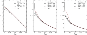
Figure 8. The effect of a component’s ellipticity on the PSF convolution, for three different Sérsic functions with the same μ e and Re but different n. All profiles represent surface brightness as a function of radius, in arbitrary units. In each panel, the thick grey curve represents the unconvolved Sérsic profile, the thick black lines (solid, dot-dashed, and dashed) represent the profile convolved in 2D with a circular Gaussian PSF, assuming different ellipticities (ε) for the Sérsic model, while the thin red curve represents the profile (incorrectly) convolved in 1D with the same PSF profile. Convolving the grey curve in 1D is inappropriate because, while it does conserve the area under grey curve [Equation (18)], it does not conserve the total flux [Equation (19)], and therefore does not model the effect of seeing. The Gaussian FWHM was chosen to be large (0.167 = 0.5Re , in the arbitrary units of the x-axis), for clarity.
Second, the PSF convolution should not be performed in 1D, i.e., by convolving the SBP curve with the PSF profile. This is because each data point in the SBP represents a (local) surface brightness at a particular distance from the centre (R) and along a particular direction (θ), i.e., I ≡ I(R, θ). The SBP itself represents the radial distribution of light for a particular choice of θ (e.g., major axis: θ = 0) and is analogous to, but more accurate than, a 1D cut from the image provided that the isophote PAs are constant with radius. As such, the area under the curve,
 $$\begin{equation}
\int _0^{\infty } I(R,\theta ){\rm d}R,
\end{equation}$$
$$\begin{equation}
\int _0^{\infty } I(R,\theta ){\rm d}R,
\end{equation}$$
does not correspond to the total flux in the image, which requires an additional integration in the azimuthal direction:
 $$\begin{equation}
\int _0^{2\pi } \int _0^{\infty } R\, I(R,\theta ) \: {\rm d}R\, {\rm d}\theta .
\end{equation}$$
$$\begin{equation}
\int _0^{2\pi } \int _0^{\infty } R\, I(R,\theta ) \: {\rm d}R\, {\rm d}\theta .
\end{equation}$$
A 1D convolution conserves the area under the SBP curve [Equation (18)] but not the total flux in the image [Equation (19)], and is therefore inappropriate to reproduce seeing effects in images, which conserve total flux. The difference between the two types of convolution (1D vs. 2D) is also illustrated in Figure 8.
The convolution is performed in several steps. If the fitting axis is the major axis, then an elliptical 2D light distribution is generated, with a global ellipticity provided by the user and the same profile along the major axis as that of the model SBP. If the fitting is performed along the equivalent axis, the convolution is performed as above except that ε c is set to 0, since the equivalent axis is circularly symmetric by construction.
In the next step, a circularly symmetric 2D PSF is generated, on the same array as the model. This can be based on either the parameters of Gaussian or Moffat forms, or the user-provided data vector PSF. The model array and PSF array are then convolved using the FFT (Fast Fourier Transform) method, and finally, the resulting distribution’s major axis profile is obtained, which represents the desired convolved model SBP. This quantity is compared with the data at each iteration.
4.2. Minimisation and solution
While most 2D decomposition codes perform signal-to-noise (S/N)-weighted minimisations in intensity units, Profiler uses an unweighted least-squares method in units of surface brightness. Because noise in galaxy images is dominated by Poisson noise, galaxies have the highest S/N at the centre, where they are usually brightest. However, the central regions can often be affected by dust, active galactic nuclei, nuclear discs, or PSF uncertainty, the latter being particularly important for highly concentrated galaxies. Therefore, placing most of the weight on the central data points can substantially bias the fit for the entire radial range if all of these issues are not dealt with (see similar arguments in Graham et al. Reference Graham, Durré, Savorgnan, Medling, Batcheldor, Scott, Watson and Marconi2016). In an unweighted scheme, all data points along the SBP contribute equally to constraining the model and thus, even when the central data is biased, the model is still well constrained by the outer data points. The caveat, however, is that one must ensure that the image sky background is accurately measured and subtracted, otherwise the outer data points introduce a bias in the model. For example, if the outer data corresponds to an exponential disc, inaccurate background subtraction would lead to the wrong scale length, which affects the entire radial range because a disc component runs all the way to the centre.
The minimisation is performed with the Python package lmfit Footnote 7 , and the method is a least-squares Levenberg–Marquardt algorithm (Marquardt Reference Marquardt1963). The quantity being minimised is
 $$\begin{equation}
\Delta _{\rm rms} = \sqrt{ \sum _i (\mu _{{\rm data},i} - \mu _{{\rm model},i })} ,
\end{equation}$$
$$\begin{equation}
\Delta _{\rm rms} = \sqrt{ \sum _i (\mu _{{\rm data},i} - \mu _{{\rm model},i })} ,
\end{equation}$$
where i is the radial bin, μdata is the data SBP, and μmodel is the model at one iteration.
When the solution is reached, the result is displayed and a logfile is generated. The logfile contains a time-stamp of the fit, all the input information and settings, and a raw fit report with all parameters and their correlations. A more in-depth report follows, which lists each component’s best-fit parameter values and, if the decomposition was performed on the equivalent axis, their total magnitude.
The quantity Δrms quantifies the global quality of the fit, but a more reliable proxy of the solution’s accuracy, in detail, is the residual profile: Δμ(R) = μdata(R) − μmodel(R). A good fit is characterised by a flat Δμ profile which scatters about the zero value with a level of scatter of the order of the noise level in the data profile. Systematic features such as curvature usually signal the need for additional components, or modelling with inadequate functions, or biased data (caused by e.g., unmasked dust). While the addition of more components will invariably improve the fit, it must nevertheless remain physically motivated, i.e., the user should seek evidence for the presence of extra components, either in the image, ellipticity, PA, or B 4 profile. As noted in Section 3.4 of Dullo & Graham (Reference Dullo and Graham2014), one should not blindly add Sérsic components.
The user can choose the radial range of data to be considered throughout the fit, by entering start and stop values (in arcsec). While excluding any data is not generally desirable (unless there are biasing factors in a particular range), particularly in the central regions, where most of the signal is, varying the radial extent of the data can provide an idea of the stability of the chosen model, and the uncertainties in its parameters.
5 EXAMPLE DECOMPOSITIONS
5.1. NGC 3348 – a cored elliptical galaxy
In the first example, I consider the galaxy NGC 3348, a massive elliptical galaxy with a cored inner SBP (Rest et al. Reference Rest, van den Bosch, Jaffe, Tran, Tsvetanov, Ford, Davies and Schafer2001, Graham et al. Reference Graham, Erwin, Trujillo and Asensio Ramos2003). Archival HST data taken with the ACS/WFC camera (F814W filter) was retrieved from the Hubble Legacy Archive Footnote 8 (Figure 9, panel a). The sky background was measured with Imexamine close to the chip edges, and subtracted from the image. The galaxy light profile was extracted from the resulting image with Isofit and the PSF was characterised from the image by fitting a Moffat profile to bright stars, with Imexamine.
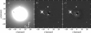
Figure 9. Panel (a): HST (F814W) image of the cored early-type galaxy NGC 3348. Panel (b): Image in (a) minus a 2D reconstruction generated with Cmodel (see Ciambur Reference Ciambur2015), based on isophote fitting with Isofit. Panel (c): Image in (a) minus a reconstruction based on the same isophote tables but with the data surface brightness column (red circles in Figure 10, top panel) replaced by the decomposition model obtained with Profiler (black curve in Figure 10, top panel). The image stretch was adjusted to reveal low small-level systematics ( < 0.05 mag arcsec−2) causing the appearence of ripples (and correspond to the curvature in the residual profile Δμ(R), also shown in Figure 10, second panel from the top). The central systematic indicates that the core region is offset from the photometric centre of the external isophotes.
The galaxy was modelled with a single core-Sérsic component, in the range 0–50 arcsec (roughly the distance from the photocentre to three out of four chip edges of the ACS/WFC chip), and the best-fitting solution is displayed in Figure 10. A 2D reconstruction of the image, with the IRAF task Cmodel, was further generated based on the isophote parameters, i.e., their surface brightness, ellipticity, and Fourier harmonics along the major axis. This reconstructed image was then subtracted from the original image, which resulted in the residual map shown in Figure 9, panel b. Panel c of the same figure shows the residual map obtained from the same isophote table but with the surface brightness column (red symbols in Figure 10) replaced with the modelled SBP (black curve in Figure 10).
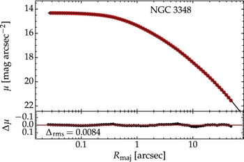
Figure 10. Major axis surface brightness profile (red circles) of the cored elliptical galaxy NGC 3842, obtained from the HST, F814W filter. The model is a core-Sérsic profile [black curve; Equation (7)], with break radius Rb = 0.43 arcsec, inner slope γ = 0.09, and break sharpness α = 1.86. The profile beyond Rb has a Sérsic index of n = 4.91 and half-light radius of Re = 27.63 arcsec. The bottom panel shows the residual profile (Δμ).
The single-component fit yielded a core radius of Rb = 0.43 arcsec, break sharpness α = 1.86, core slope γ = 0.09, half-light radius Re = 27.63 arcsec, and Sérsic index n = 4.91. These results are generally in good agreement with Graham et al. (Reference Graham, Erwin, Trujillo and Asensio Ramos2003), though the outer Sérsic parameters, Re and n, are both ~ 21% higher in this analysis. The break radius agrees well with their reported value of Rb = 0.45 arcsec, whereas the inner profile slope is shallower in this work than their reported value of γ = 0.18.
When interpreting these differences it must be taken into consideration that this analysis was performed on different imaging than the WFPC2/F555W data used in Graham et al. (Reference Graham, Erwin, Trujillo and Asensio Ramos2003). The ACS/WFC/F814W image was preferred in this instance due to its better spatial resolution and lower sensitivity to dust. Both aspects are important when probing small-scale structures like depleted cores. Additionally, and perhaps more importantly, Graham et al. (Reference Graham, Erwin, Trujillo and Asensio Ramos2003) performed the decomposition on deconvolved data from Rest et al. (Reference Rest, van den Bosch, Jaffe, Tran, Tsvetanov, Ford, Davies and Schafer2001), whereas Profiler accounts for seeing effects by convolving the model instead. As Ferrarese et al. (Reference Ferrarese, Cote, Blakeslee, Mei, Merritt and West2006) point out, deconvolving (noisy) data can lead to unstable results, as it is sensitive to noise and contamination from bright sources or dust. This can have a significant impact on small-scale features such as core regions. On the other hand, the convolution of a noisless model is mathematically a more well-defined process, and hence is more robust. Profiler’s convolution scheme was tested with Sérsic and core-Sérsic models and Gaussian seeing, by modelling synthetic 2D images with known light profiles, that were generated and convolved with independent software (the IRAF tasks Bmodel and Gauss).
The core-Sérsic model was tested with Profiler on four additional cored galaxies (namely NGC 1016, NGC 3842, NGC 5982, and NGC 7619) and compared with results from Dullo & Graham (Reference Dullo and Graham2012) and Dullo & Graham (Reference Dullo and Graham2014). These works, like Graham et al. Reference Graham, Erwin, Trujillo and Asensio Ramos2003, have used deconvolved profiles, but taken from Lauer et al. (Reference Lauer2005). The core slopes obtained with Profiler were systematically shallower (Δγ ~ 0.05–0.25) than the literature values computed from deconvolved dataFootnote 9 . If this is indeed a systematic discrepancy and not simply a chance occurrence in the five galaxies considered here, this issue would imply that literature measurements of the cores’ light deficit are biased-low, if the Profiler result is indeed the correct one. This is probably the case, considering that (i) Profiler accounts for seeing by convolving the model—a more robust approach than fitting deconvolved, noisy data; (ii) the convolution scheme was tested with independent software; and (iii) many literature results are based on deconvolved data and fits where the α parameter is not allowed to vary. In order to confirm this discrepancy and identify its causes, a more comprehensive study on a larger sample of cored galaxies would be necessary, which is however beyond the scope of this paper.
5.2. Pox 52—using the data vector PSF option
The second example is intended to illustrate how, when diffraction effects are significant, even the Moffat approximation of the true PSF is inadequate and can lead to wrong results. This can be avoided with Profiler through the use of the data vector PSF feature.
The data chosen for demonstrating this feature was an HST image of the nucleated dwarf Seyfert 1 galaxy Pox 52 (Kunth, Sargent, & Bothun Reference Kunth, Sargent and Bothun1987, Barth et al. Reference Barth, Ho, Rutledge and Sargent2004, Thornton et al. Reference Thornton, Barth, Ho, Rutledge and Greene2008), observed with the ACS/HRC camera in the I − band (F814W filter).
The bright point-source (AGN) at the centre is ‘spread’ onto the detector into a distinct Airy pattern (see Figure 11), which is also obvious in the SBP (Figure 12). For this galaxy, the PSF was characterised from a bright, nearby star (inset of Figure 11), in two ways: (a) by fitting a Moffat profile with Imexamine and (b) by fitting the star’s light profile (extracted with Ellipse) with four Gaussians (for the Airy disc and first three rings)Footnote 10 . The galaxy’s SBP was then fit with Profiler with two components, namely a nuclear point source and a Sérsic component. This was done for both PSF choices, and the results are displayed in Figure 12.
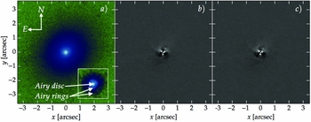
Figure 11. I-band image of Pox 52, taken with the ACS/HRC camera (F814W filter) onboard the HST. The three panels are analogous to Figure 4, except panel (a) is plotted on a logarithmic scale and false-colour scheme, for clarity. With a pixel size of 0.025 arcsec, the PSF is well sampled: The central point source displays a clear first Airy ring and a faint second. The Airy rings are also obvious in the surface brightness profile (Figure 12). The inset is a nearby bright star in the same data, to the SW of Pox 52. For clarity, it is zoomed-in by a ratio of 2:1 compared to the Pox 52 image.
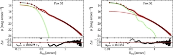
Figure 12. Equivalent axis surface brightness profile of Pox 52 (red circles) modelled with two choices of PSF: a Moffat PSF (left-hand panel) and a data vector PSF (right-hand panel). The models (black curves) are each built from a point-source (green) and a Sérsic component (red). The data vector PSF better captures the Airy rings (see Figure 11) and thus provides a superior model.
The best-fitting Moffat profile from Imexamine had an FWHM of 3.04 pixels and a β parameter of 7.41. The high value of β indicates that Imexamine fit essentially a Gaussian on just the Airy disc (first peak of the PSF) and ignored the wings (Airy rings)Footnote 11 .
The decomposition solution with the Moffat PSF is a two-component model: a point source of central surface brightness μ0 = 13.51 and a Sérsic component characterised by μ e = 19.62, Re = 1.03 arcsec, and n = 4.19. This solution is displayed in the left-hand panel of Figure 11. During the decomposition process, Profiler tried to compensate for the unaccounted-for flux in the PSF wings (between 0.1–0.3 arcsec) by making the Sérsic component more concentrated than it should be. This illustrates a case when things went wrong, not because of Profiler but because of the input PSF.
When performing the decomposition with a data vector PSF, the flux in the wings of the PSF is accounted for much more accurately, and the overall solution is better. Quantitatively, it was also a two-component model, with the point source μ0 = 12.92 and the Sérsic component μ e = 20.11, Re = 1.27 arcsec, and n = 3.12. The Sérsic component is now less concentrated and its total magnitude m = 16.33 mag (in the Vega magnitude system) is ~ 50% fainter than in the previous case, but in good agreement with the value of 16.2 reported by Thornton et al. (Reference Thornton, Barth, Ho, Rutledge and Greene2008). Additionally, the residual profile displays considerably reduced curvature beyond 0.1arcsec (Δrms is reduced by a factor of 2), though there is still systematic curvature at the scale of the first two Airy rings, which is due to the still imperfect PSF estimation.
5.3. NGC 2549 – one spheroid, two bars, and a truncated disc
The third example involves the complex edge-on galaxy NGC 2549. Apart from a spheroid and a disc component, this object shows the signatures of two nested bars, and was shown to host nested X/peanut-shaped structures associated with the two bars (Ciambur & Graham Reference Ciambur and Graham2016).
SDSS r-band data from DR9 (Figure 13, panel a) was analysed as before, and the best-fitting model consisted of a Sérsic shperoid, two nested bars, also modelled with Sérsic functions, and a truncated (Type II) exponential disc, with a break radius of 86.2 arcsec, inner scale length h1 = 42.7 arcsec and outer h2 = 27.2. The solution is displayed in Figure 14, which also shows the ellipticity and B 4 harmonic profiles. Displaying these ancillary profiles is an option available to the user (as check-boxes in the GUI, see Figure 1) and, in conjunction with the residual profile, they are often useful to signal the presence of additional components—in this case, both ε(R maj) and B 4(R maj) strongly indicate the presence of the inner bar component, and also display faint ‘bumps’ corresponding to the outer bar, which is however more obvious in the SBP. The detection of the nested bars is particularly important given that this galaxy is viewed edge-on, i.e., the most difficult orientation for finding bars.
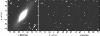
Figure 13. Panel (a): SDSS r − band image of NGC 2549. Panel (b): Image in (a) minus a 2D reconstruction generated with Cmodel (see Ciambur Reference Ciambur2015), based on isophote fitting with Isofit. Panel (c): Image in (a) minus a 2D reconstruction with Cmodel, based on the same isophote tables but with the data surface brightness column (red circles in Figure 14, top panel) replaced by decomposition model obtained with Profiler (black curve in Figure 14, top panel). The image stretch was adjusted to reveal low-level systematics, which cause the appearence of ripples (and correspond to the curvature in the residual profile Δμ(R), also shown in Figure 14, second panel from the top). However, the nested peanut structures are well captured (there are no X-shaped systematics).
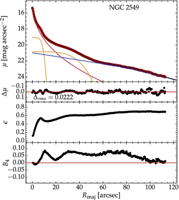
Figure 14. Top panel shows the major axis surface brightness profile decomposition of the edge-on, double-bar (nested peanut) galaxy NGC 2549, based on SDSS r-band data. The model is made up of a Sérsic spheroid (red), two nested, Sérsic bars (orange; n = 0.15 for the inner, n = 0.23 for the outer) and a truncated disc (blue) with a truncation radius of Rb = 86 arcsec. Directly underneath is he residual profile, followed by the ellipticity (ε) and B 4 (boxyness/discyness) profiles.
As before, a 2D reconstruction of the galaxy image was performed with Cmodel, based on the best-fitting SBP and the isophote parameters computed by Isofit. This was subtracted from the original galaxy image, resulting in a residual image displayed in Figure 13, panel (c). The appearence of waves in-a-pond reflects the curvature in the residual profile Δμ (Figure 14). Note, however, that there are no X-shaped systematics, which indicates that the peanut bulges were well captured by the isophotal analysis.
6 CONCLUSIONS
I have introduced Profiler, a flexible and user-friendly programme coded in Python, designed to model radial SBP of galaxies.
With an intuitive GUI, Profiler can model a wide range of galaxy components, such as elliptical galaxies or the bulges of spiral or lenticular galaxies, face-on, inclined, edge-on, and (anti-)truncated discs, resolved or unresolved nuclear point-sources, bars, rings, or spiral arms, with an arsenal of analytical functions routinely used in the field. These include the Sérsic and core-Sérsic functions, the edge-on disc model, the exponential, Gaussian, Moffat, and Ferrers’ functions. In addition, Profiler can employ a broken exponential model (relevant for disc truncations or anti-truncations) and two 1D special cases of the 2D edge-on disc model, namely along the major axis and along the minor axis.
Profiler is optimised to analyse isophote tables generated by the IRAF tasks Ellipse and Isofit but can also analyse two-column tables of radius and surface brightness. After reaching the best-fitting solution, the corresponding model parameters are returned. The major and equivalent axis profiles can both be analysed, and for the latter profile, each component’s total magnitude is additionally returned.
The model convolution with the PSF is performed in 2D, with a FFT-based scheme. This allows for elliptical models, and additionally ensures that the convolution conserves the model’s total flux (as a 1D convolution of the model profile with the PSF profile does not). Further, Profiler allows for a choice between Gaussian, Moffat, or a user-provided data vector for the PSF (a table of R and I(R) values). All of the possible PSF choices can also be used as point-source components in the model.
Profiler is freely available from the following URL: https://github.com/BogdanCiambur/PROFILER.
ACKNOWLEDGEMENTS
I am grateful to A. Graham for teaching me the subtleties of galaxy decomposition, and for reading parts of this manuscript. I also thank the anonymous referee for helpful comments, and G. Savorgnan and B. Dullo for useful discussions. Funding for SDSS-III has been provided by the Alfred P. Sloan Foundation, the Participating Institutions, the National Science Foundation, and the U.S. Department of Energy Office of Science. Part of this work is based on observations made with the NASA/ESA Hubble Space Telescope, and obtained from the Hubble Legacy Archive, which is a collaboration between the Space Telescope Science Institute (STScI/NASA), the Space Telescope European Coordinating Facility (ST-ECF/ESA), and the Canadian Astronomy Data Centre (CADC/NRC/CSA).