


1. Introduction
Active galactic nuclei (AGNs), the most luminous objects with supermassive black holes lurking at their centres, are among the most energetic sources in the universe and play a crucial role in the evolution of galaxies. Blazars, as the most extreme subclass of AGNs with a radio-loud behaviour and a relativistic jet pointing towards the observer (Urry & Padovani Reference Urry and Padovani1995), are characterised by having large amplitude and rapid variability, superluminal motion, high polarisation, core-dominated non-thermal continuum, and  $\gamma$
-ray emission, etc. (Wills et al. Reference Wills, Wills, Breger, Antonucci and Barvainis1992; Fan & Xie Reference Fan and Xie1996; Bai et al. Reference Bai, Xie, Li, Zhang and Liu1998; Romero et al. Reference Romero, Cellone, Combi and Andruchow2002; Fan Reference Fan2005; Fan et al. Reference Fan, Yang, Pan and Hua2011, Reference Fan, Yang, Zhang, Hua, Liu, Qin and Huang2013b, Reference Fan2016; Ghisellini et al. Reference Ghisellini, Tavecchio, Foschini, Ghirlanda, Maraschi and Celotti2010; Abdo et al. Reference Abdo2009; Abdo et al. Reference Abdo2010b,c; Urry Reference Urry2011; Marscher et al. Reference Marscher, Jorstad, Larionov, Aller and Lähteenmäki2011; Nolan et al. Reference Nolan2012; Yang, Fan, & Yuan Reference Yang, Fan and Yuan2012; Yang et al. Reference Yang, Fan, Zhang, Yang, Tuo and Nie2019; Gupta et al. Reference Gupta2012; Acero et al. Reference Acero2015; Xiao et al. Reference Xiao2019; Ajello et al. Reference Ajello2020; Pei et al. Reference Pei, Fan, Bastieri, Sawangwit and Yang2019, Reference Pei, Fan, Bastieri, Yang, Xiao and Yang2020a,b). All of these properties are due to the relativistic beaming effect. The emissions in the jet are highly boosted along the line of the observer’s sight. The spectral energy distribution (SED) of the broadband continuum emission (from radio to
$\gamma$
-ray emission, etc. (Wills et al. Reference Wills, Wills, Breger, Antonucci and Barvainis1992; Fan & Xie Reference Fan and Xie1996; Bai et al. Reference Bai, Xie, Li, Zhang and Liu1998; Romero et al. Reference Romero, Cellone, Combi and Andruchow2002; Fan Reference Fan2005; Fan et al. Reference Fan, Yang, Pan and Hua2011, Reference Fan, Yang, Zhang, Hua, Liu, Qin and Huang2013b, Reference Fan2016; Ghisellini et al. Reference Ghisellini, Tavecchio, Foschini, Ghirlanda, Maraschi and Celotti2010; Abdo et al. Reference Abdo2009; Abdo et al. Reference Abdo2010b,c; Urry Reference Urry2011; Marscher et al. Reference Marscher, Jorstad, Larionov, Aller and Lähteenmäki2011; Nolan et al. Reference Nolan2012; Yang, Fan, & Yuan Reference Yang, Fan and Yuan2012; Yang et al. Reference Yang, Fan, Zhang, Yang, Tuo and Nie2019; Gupta et al. Reference Gupta2012; Acero et al. Reference Acero2015; Xiao et al. Reference Xiao2019; Ajello et al. Reference Ajello2020; Pei et al. Reference Pei, Fan, Bastieri, Sawangwit and Yang2019, Reference Pei, Fan, Bastieri, Yang, Xiao and Yang2020a,b). All of these properties are due to the relativistic beaming effect. The emissions in the jet are highly boosted along the line of the observer’s sight. The spectral energy distribution (SED) of the broadband continuum emission (from radio to  $\gamma$
-ray) of blazars are usually dominated by two spectral bumps. The low-energy bump, from radio through optical/UV (X-rays, in some cases), ascribes to the synchrotron emission from the relativistic electrons in the jet. The second bump, located in the high energy (X-ray through
$\gamma$
-ray) of blazars are usually dominated by two spectral bumps. The low-energy bump, from radio through optical/UV (X-rays, in some cases), ascribes to the synchrotron emission from the relativistic electrons in the jet. The second bump, located in the high energy (X-ray through  $\gamma$
-ray), is believed to be emanated from the inverse Compton scattering of low-energy photons. According to the optical spectral features, blazars are grouped into flat-spectrum radio quasars (FSRQs) and BL Lac objects (BL Lacs) (Scarpa & Falomo Reference Scarpa and Falomo1997). A more physical classification between FSRQs and BL Lacs can be distinguished via their SED synchrotron peak frequencies
$\gamma$
-ray), is believed to be emanated from the inverse Compton scattering of low-energy photons. According to the optical spectral features, blazars are grouped into flat-spectrum radio quasars (FSRQs) and BL Lac objects (BL Lacs) (Scarpa & Falomo Reference Scarpa and Falomo1997). A more physical classification between FSRQs and BL Lacs can be distinguished via their SED synchrotron peak frequencies  $\log \, \nu_{p}$
. Low-synchrotron peaked (LSP) blazars are characterised by
$\log \, \nu_{p}$
. Low-synchrotron peaked (LSP) blazars are characterised by  $\log \, \nu_{p}$
(Hz) < 14, and intermediate-synchrotron peaked(ISP) blazars have 14 <
$\log \, \nu_{p}$
(Hz) < 14, and intermediate-synchrotron peaked(ISP) blazars have 14 <  $\log \, \nu_{p}$
(Hz) < 15, while
$\log \, \nu_{p}$
(Hz) < 15, while  $\log \, \nu_{p}$
(Hz) > 15 pertains to high-synchrotron peaked (HSP) blazars. The majority of ISP and HSP blazars have been classified as BL Lacs, while LSP ones include FSRQs and some low-frequency-peaked BL Lacs (see Abdo et al. Reference Abdo2010c; Fan et al. Reference Fan2016; Böttcher Reference Böttcher2019, and references therein).
$\log \, \nu_{p}$
(Hz) > 15 pertains to high-synchrotron peaked (HSP) blazars. The majority of ISP and HSP blazars have been classified as BL Lacs, while LSP ones include FSRQs and some low-frequency-peaked BL Lacs (see Abdo et al. Reference Abdo2010c; Fan et al. Reference Fan2016; Böttcher Reference Böttcher2019, and references therein).
Based on a relativistic beaming model, Urry & Shafer (Reference Urry and Shafer1984) proposed that the total emission from AGNs is from two components, namely, a beamed component (core component) and an unbeamed one (extended component). Then, the observed total luminosity,  $L^{\rm tot}$
, is the sum of the beamed,
$L^{\rm tot}$
, is the sum of the beamed,  $L_{\textrm{b}}$
, and unbeamed,
$L_{\textrm{b}}$
, and unbeamed,  $L_{\textrm{unb}}$
emissions, that is,
$L_{\textrm{unb}}$
emissions, that is,  $L^{\rm tot}=L_{\textrm{b}}+L_{\textrm{unb}}$
. In the radio band, the ratio of the two components, R, is defined as the core-dominance parameter, that is,
$L^{\rm tot}=L_{\textrm{b}}+L_{\textrm{unb}}$
. In the radio band, the ratio of the two components, R, is defined as the core-dominance parameter, that is,  $R=L_{\textrm{b}}/L_{\textrm{unb}}$
(see Orr & Browne Reference Orr and Browne1982; Fan et al. Reference Fan, Yang, Pan and Hua2011; Pei et al. Reference Pei2016, Reference Pei, Fan, Bastieri, Sawangwit and Yang2019, Reference Pei, Fan, Bastieri, Yang, Xiao and Yang2020a,b, and references therein) and also can be expressed as
$R=L_{\textrm{b}}/L_{\textrm{unb}}$
(see Orr & Browne Reference Orr and Browne1982; Fan et al. Reference Fan, Yang, Pan and Hua2011; Pei et al. Reference Pei2016, Reference Pei, Fan, Bastieri, Sawangwit and Yang2019, Reference Pei, Fan, Bastieri, Yang, Xiao and Yang2020a,b, and references therein) and also can be expressed as  $R=S_{\textrm{core}}/S_{\textrm{ext}}$
, where
$R=S_{\textrm{core}}/S_{\textrm{ext}}$
, where  $S_{\textrm{core}}$
and
$S_{\textrm{core}}$
and  $S_{\textrm{ext}}$
refer to the flux density derived from the core and the extended components of radio emission.
$S_{\textrm{ext}}$
refer to the flux density derived from the core and the extended components of radio emission.
In addition, due to the relativistic beaming effect, the emissions from the jet are strongly boosted in the observer’s frame, that is,  $S^{\rm ob}=\delta^{p}S^{\rm in}$
, where
$S^{\rm ob}=\delta^{p}S^{\rm in}$
, where  $S^{\rm ob}$
is the observed emission,
$S^{\rm ob}$
is the observed emission,  $S^{\rm in}$
is the intrinsic emission in the source frame, and
$S^{\rm in}$
is the intrinsic emission in the source frame, and  $\delta$
is the Doppler factor. The value of p hinges on the physical detail of the jet and geometrical shape of the emitted spectrum (Lind & Blandford Reference Lind and Blandford1985),
$\delta$
is the Doppler factor. The value of p hinges on the physical detail of the jet and geometrical shape of the emitted spectrum (Lind & Blandford Reference Lind and Blandford1985),  $p=2+\alpha$
for continuous jet while
$p=2+\alpha$
for continuous jet while  $p=3+\alpha$
for a moving compact source,
$p=3+\alpha$
for a moving compact source,  $\alpha$
is the spectral index (
$\alpha$
is the spectral index ( $f_{\nu}\propto \nu^{-\alpha}$
).
$f_{\nu}\propto \nu^{-\alpha}$
).
The Doppler boosting factor can be expressed by  $\delta=[\Gamma(1-\beta\cos\theta)]^{-1}$
, where
$\delta=[\Gamma(1-\beta\cos\theta)]^{-1}$
, where  $\Gamma$
is a Lorentz factor (
$\Gamma$
is a Lorentz factor ( $\Gamma=1/\sqrt{1-\beta^{2}}$
),
$\Gamma=1/\sqrt{1-\beta^{2}}$
),  $\beta$
is the jet speed in units of the speed of light and
$\beta$
is the jet speed in units of the speed of light and  $\theta$
is the viewing angle between the jet and the line of sight. The Doppler factor is a crucial parameter in the jet of blazars since it reckons how strongly the flux densities are boosted and timescales compressed in the observer’s frame. However, it is difficult for us to determine this parameter since it is unobservable. Therefore, some feasible methods have been proposed (Ghisellini et al. Reference Ghisellini, Padovani, Celotti and Maraschi1993; Mattox et al. Reference Mattox1993; Lähteenmäki & Valtaoja Reference Lähteenmäki and Valtaoja1999; Fan et al. Reference Fan, Huang, He, Yang, Hua, Liu and Wang2009; Hovatta et al. Reference Hovatta, Valtaoja, Tornikoski and Lähteenmäki2009; Liodakis et al. Reference Liodakis, Hovatta, Huppenkothen, Kiehlmann, Max-Moerbeck and Readhead2018; Zhang et al. Reference Zhang, Chen, Xiao, Cai and Fan2020).
$\theta$
is the viewing angle between the jet and the line of sight. The Doppler factor is a crucial parameter in the jet of blazars since it reckons how strongly the flux densities are boosted and timescales compressed in the observer’s frame. However, it is difficult for us to determine this parameter since it is unobservable. Therefore, some feasible methods have been proposed (Ghisellini et al. Reference Ghisellini, Padovani, Celotti and Maraschi1993; Mattox et al. Reference Mattox1993; Lähteenmäki & Valtaoja Reference Lähteenmäki and Valtaoja1999; Fan et al. Reference Fan, Huang, He, Yang, Hua, Liu and Wang2009; Hovatta et al. Reference Hovatta, Valtaoja, Tornikoski and Lähteenmäki2009; Liodakis et al. Reference Liodakis, Hovatta, Huppenkothen, Kiehlmann, Max-Moerbeck and Readhead2018; Zhang et al. Reference Zhang, Chen, Xiao, Cai and Fan2020).
From the previous studies, the core-dominance parameter R can take the role of the indicator of Doppler-boosted beaming effect (see Urry & Padovani Reference Urry and Padovani1995; Fan Reference Fan2003):
 \begin{equation}R = f_{\textrm{in}} \Gamma^{-n}[(1 - \beta \cos \theta)^{-n + \alpha} + (1 + \beta \cos \theta)^{-n + \alpha}],\end{equation}
where  $f_{\textrm{in}}$
is a ratio, defined by the intrinsic flux density in the jet to the extended flux density in the co-moving frame,
$f_{\textrm{in}}$
is a ratio, defined by the intrinsic flux density in the jet to the extended flux density in the co-moving frame,  $f_{\textrm{in}} = \frac{S^{\rm in}_{\textrm{core}}}{S^{\rm in}_{\textrm{ext.}}}$
,
$f_{\textrm{in}} = \frac{S^{\rm in}_{\textrm{core}}}{S^{\rm in}_{\textrm{ext.}}}$
,  $\alpha$
is the spectral index, and n = 2 or 3.
$\alpha$
is the spectral index, and n = 2 or 3.
After the launch of Fermi Large Area Telescope (hereafter, Fermi/LAT), many new high-energy  $\gamma$
-ray sources were detected, revolutionising, in particular, the knowledge of
$\gamma$
-ray sources were detected, revolutionising, in particular, the knowledge of  $\gamma$
-ray blazars, providing us with the opportunity to study the
$\gamma$
-ray blazars, providing us with the opportunity to study the  $\gamma$
-ray production mechanism. Based on the first 8 yr of data from the Fermi Gamma-ray Space Telescope mission, the latest catalogue, 4FGL, or the fourth Fermi Large Area Telescope catalogue of high-energy
$\gamma$
-ray production mechanism. Based on the first 8 yr of data from the Fermi Gamma-ray Space Telescope mission, the latest catalogue, 4FGL, or the fourth Fermi Large Area Telescope catalogue of high-energy  $\gamma$
-ray sources, has been released, which includes 5 098 sources above the significance of
$\gamma$
-ray sources, has been released, which includes 5 098 sources above the significance of  $4\sigma$
, covering the 50 MeV
$4\sigma$
, covering the 50 MeV $-$
1 TeV range (Abdollahi et al. Reference Abdollahi2020; Ajello et al. Reference Ajello2020), about 2 000 more than the previous 3FGL catalogue (Acero et al. Reference Acero2015). AGNs are the vast majority of sources in 4FGL; among them 2 938 blazars, or 681 FSRQs, 1 102 BL Lacs and 1 152 blazar candidates of unknown class (BCUs, Abdollahi et al. Reference Abdollahi2020).
$-$
1 TeV range (Abdollahi et al. Reference Abdollahi2020; Ajello et al. Reference Ajello2020), about 2 000 more than the previous 3FGL catalogue (Acero et al. Reference Acero2015). AGNs are the vast majority of sources in 4FGL; among them 2 938 blazars, or 681 FSRQs, 1 102 BL Lacs and 1 152 blazar candidates of unknown class (BCUs, Abdollahi et al. Reference Abdollahi2020).
The previous studies have probed the correlation between  $\gamma$
-ray emission and radio emission for the selected
$\gamma$
-ray emission and radio emission for the selected  $\gamma$
-ray loud blazars and showed that the
$\gamma$
-ray loud blazars and showed that the  $\gamma$
-ray emission is strongly beamed (Dondi & Ghisellini Reference Dondi and Ghisellini1995; Fan et al. Reference Fan, Adam, Xie, Cao, Lin and Copin1998). Consequently, the
$\gamma$
-ray emission is strongly beamed (Dondi & Ghisellini Reference Dondi and Ghisellini1995; Fan et al. Reference Fan, Adam, Xie, Cao, Lin and Copin1998). Consequently, the  $\gamma$
-ray Doppler factor (
$\gamma$
-ray Doppler factor ( $\delta_{\gamma}$
) can be estimated for each
$\delta_{\gamma}$
) can be estimated for each  $\gamma$
-ray loud blazars accordingly (Fan, Xie, & Bacon Reference Fan, Xie and Bacon1999; Fan Reference Fan2005).
$\gamma$
-ray loud blazars accordingly (Fan, Xie, & Bacon Reference Fan, Xie and Bacon1999; Fan Reference Fan2005).
Pei et al. (Reference Pei, Fan, Bastieri, Sawangwit and Yang2019) had compiled a catalogue listing 2 400 AGNs with available core-dominance parameters ( $\log \, R$
), 770 of which are blazars. It was found that blazars have, on average, higher
$\log \, R$
), 770 of which are blazars. It was found that blazars have, on average, higher  $\log \, R$
than those non-blazars objects, indicating that blazars are more core-dominated (see also Fan et al. Reference Fan, Yang, Pan and Hua2011). Pei et al. (Reference Pei, Fan, Bastieri, Yang and Xiao2020b) analysed a larger sample of 4 388 AGNs with available
$\log \, R$
than those non-blazars objects, indicating that blazars are more core-dominated (see also Fan et al. Reference Fan, Yang, Pan and Hua2011). Pei et al. (Reference Pei, Fan, Bastieri, Yang and Xiao2020b) analysed a larger sample of 4 388 AGNs with available  $\log \, R$
, 584 are Fermi/LAT-detected blazars from 4FGL, and obtained that the
$\log \, R$
, 584 are Fermi/LAT-detected blazars from 4FGL, and obtained that the  $\langle\log R\rangle$
for Fermi blazars is higher than that for non- Fermi-detected blazars. This is the evidence that the
$\langle\log R\rangle$
for Fermi blazars is higher than that for non- Fermi-detected blazars. This is the evidence that the  $\gamma$
-ray emission is strongly beamed (Ghisellini et al. Reference Ghisellini, Padovani, Celotti and Maraschi1993; Dondi & Ghisellini Reference Dondi and Ghisellini1995; Fan et al. Reference Fan, Yang, Zhang, Hua, Liu, Qin and Huang2013b; Pei et al. Reference Pei2016).
$\gamma$
-ray emission is strongly beamed (Ghisellini et al. Reference Ghisellini, Padovani, Celotti and Maraschi1993; Dondi & Ghisellini Reference Dondi and Ghisellini1995; Fan et al. Reference Fan, Yang, Zhang, Hua, Liu, Qin and Huang2013b; Pei et al. Reference Pei2016).
In this paper, we estimate the lower limit on  $\gamma$
-ray Doppler factors for those
$\gamma$
-ray Doppler factors for those  $\gamma$
-ray blazars following Mattox et al. (Reference Mattox1993) as did in Fan et al. (Reference Fan, Yang, Liu and Zhang2013a, Reference Fan, Bastieri, Yang, Liu, Hua, Yuan and Wu2014), probing their relations and shedding new light on the relativistic beaming effect of
$\gamma$
-ray blazars following Mattox et al. (Reference Mattox1993) as did in Fan et al. (Reference Fan, Yang, Liu and Zhang2013a, Reference Fan, Bastieri, Yang, Liu, Hua, Yuan and Wu2014), probing their relations and shedding new light on the relativistic beaming effect of  $\gamma$
-ray loud blazars. The methodology is discussed in Section 2, while in Section 3 we describe the sample and results. In Section 4, we present the statistical analysis and make the discussion. Finally, we draw the conclusions in Section 5. Throughout this paper, we apply the
$\gamma$
-ray loud blazars. The methodology is discussed in Section 2, while in Section 3 we describe the sample and results. In Section 4, we present the statistical analysis and make the discussion. Finally, we draw the conclusions in Section 5. Throughout this paper, we apply the  $\Lambda$
CDM model, with
$\Lambda$
CDM model, with  $\Omega_{\Lambda} \simeq 0.73$
,
$\Omega_{\Lambda} \simeq 0.73$
,  $\Omega_{M} \simeq 0.27$
, and
$\Omega_{M} \simeq 0.27$
, and  $H_{0} \simeq 73\, \rm {km \cdot s^{-1} \cdot Mpc^{-1}}$
.
$H_{0} \simeq 73\, \rm {km \cdot s^{-1} \cdot Mpc^{-1}}$
.
2. Methodology
The extreme observation properties of blazars, for example, rapid variability, high  $\gamma$
-ray luminosity, core-emission-dominated, and superluminal motion, is believed to be in connection with the relativistic beaming model. The high-energy
$\gamma$
-ray luminosity, core-emission-dominated, and superluminal motion, is believed to be in connection with the relativistic beaming model. The high-energy  $\gamma$
-ray emission detected from blazars indicate that the
$\gamma$
-ray emission detected from blazars indicate that the  $\gamma$
-rays should be strongly beamed, otherwise the
$\gamma$
-rays should be strongly beamed, otherwise the  $\gamma$
-rays would have been absorbed by the lower-energy photons due to pair production in the collision. Following the idea of Mattox et al. (Reference Mattox1993), and as did in Fan et al. (Reference Fan, Yang, Liu and Zhang2013a, Reference Fan, Bastieri, Yang, Liu, Hua, Yuan and Wu2014), we assume that:
$\gamma$
-rays would have been absorbed by the lower-energy photons due to pair production in the collision. Following the idea of Mattox et al. (Reference Mattox1993), and as did in Fan et al. (Reference Fan, Yang, Liu and Zhang2013a, Reference Fan, Bastieri, Yang, Liu, Hua, Yuan and Wu2014), we assume that:
(i) X-ray is produced in the same region as $\gamma$
-ray, and the intensities of X-ray and
$\gamma$
-ray are semblable when
$\gamma$
-ray emission is observed;
$\gamma$
-ray, and the intensities of X-ray and
$\gamma$
-ray are semblable when
$\gamma$
-ray emission is observed;(ii) the emission region is spherical;
(iii) the emission is isotropic, and the size of the emission region is constrained by the timescale of variability,
$\Delta T$
, to be less than
$R_{\textrm{size}}=c\delta\Delta T/(1+z)$
, where c is the speed of light,
$\delta$
is the Doppler factor, and z denotes the redshift, we derive the optical depth for the pair production (Mattox et al. Reference Mattox1993):
(2)where
\begin{equation}\begin{aligned}\tau&=2\times10^{3}\left[(1+z)/\delta\right]^{4+2\alpha}\left(1+z-\sqrt{1+z}\right)^{2}h_{75}^{-2}\Delta T_{5}^{-1} \\&\qquad\qquad\qquad\qquad\qquad\qquad\qquad\times\displaystyle\frac{F_{\textrm{1\,keV}}}{\mu \rm Jy}\left(\frac{E_{\gamma}}{\rm GeV}\right)^{\alpha}\!,\end{aligned}\end{equation}
$\alpha$
is the X-ray spectral index (
$F_{\nu X}\propto\nu_{X}^{-\alpha}$
),
$h_{75}=\textit{H}_{0}$
/75,
$\Delta T_{5}=\Delta T/(10^{5})$
s,
$\Delta T$
is the timescale in units of hour,
$F_{\textrm{1\,keV}}$
is the flux density at 1 keV in units of
$\mu$
Jy, and
$E_{\gamma}$
denotes the
$\gamma$
-ray photon energy in units of GeV. As the luminosity distance in units of Mpc can be expressed in the form:
(3)then the optical depth
\begin{equation}d_{L}=\displaystyle\frac{c}{H_{o}}\int^{1+z}_{1}\frac{dx}{\sqrt{\Omega_{M}x^{3}+1-\Omega_{M}}},\end{equation}
$\tau$
can be rewritten into:
(4)(Fan et al. Reference Fan, Yang, Liu and Zhang2013a). Therefore, the lower limit on
\begin{equation}\begin{aligned}\tau=1.54\times10^{-3}\displaystyle\left(\frac{1+z}{\delta}\right)^{4+2\alpha}\left(\frac{d_{L}}{\rm Mpc}\right)^{2}\left(\frac{\Delta T}{\rm h}\right)^{-1} \\\left(\frac{F_{\text{1\,keV}}}{\mu \rm Jy}\right)\left(\frac{E_{\gamma}}{\rm GeV}\right)^{\alpha}\end{aligned}\end{equation}
$\gamma$
-ray Doppler factor can be estimated if we assume that the optical depth does not exceed unity: (5)(Mattox et al. Reference Mattox1993; Fan et al. Reference Fan, Yang, Liu and Zhang2013a, Reference Fan, Bastieri, Yang, Liu, Hua, Yuan and Wu2014).
\begin{equation}\begin{aligned}\delta_{\gamma}&\ge\left[{1.54\times10^{-3}\displaystyle\left(1+z\right)^{4+2\alpha}\left(\frac{d_{L}}{\rm Mpc}\right)^{2}\left(\frac{\Delta T}{\rm h}\right)^{-1}} \right. \\&\quad\left. \left(\frac{F_{\textrm{1\,keV}}}{\mu \rm Jy}\right){\left(\frac{E_{\gamma}}{\rm GeV}\right)^{\alpha}}\right]^{\frac{1}{4+2\alpha}}\end{aligned}\end{equation}


The lower limit on  $\gamma$
-ray Doppler factor
$\gamma$
-ray Doppler factor  $\delta_{\gamma}$
can be calculated if the knowledge of the luminosity distance
$\delta_{\gamma}$
can be calculated if the knowledge of the luminosity distance  $d_{L}$
and redshift z, X-ray behaviour (characterised by the spectral index
$d_{L}$
and redshift z, X-ray behaviour (characterised by the spectral index  $\alpha_{X}$
and flux density
$\alpha_{X}$
and flux density  $F_{\textrm{1\,keV}}$
),
$F_{\textrm{1\,keV}}$
),  $\gamma$
-ray behaviour (characterised by the average
$\gamma$
-ray behaviour (characterised by the average  $\gamma$
-ray photon energy
$\gamma$
-ray photon energy  $E_{\gamma}$
), and the timescale of variation
$E_{\gamma}$
), and the timescale of variation  $\Delta T$
are given.
$\Delta T$
are given.
3. Sample and results
3.1. Sample
We compiled a catalogue of 809 Fermi-detected blazars based on the 4FGL with available X-ray data and present their derived lower limit on  $\gamma$
-ray Doppler factors in this work.
$\gamma$
-ray Doppler factors in this work.
For probing the origin of X-ray emission, Yang et al. (Reference Yang, Fan, Zhang, Yang, Tuo and Nie2019) collected 660  $\gamma$
-ray loud blazars from Fan et al. (Reference Fan2016) with available X-ray data, which contained 269 FSRQs and 391 BL Lacs, to investigate the contributions from the synchrotron radiation and inverse Compton scattering to the X-ray emission in the
$\gamma$
-ray loud blazars from Fan et al. (Reference Fan2016) with available X-ray data, which contained 269 FSRQs and 391 BL Lacs, to investigate the contributions from the synchrotron radiation and inverse Compton scattering to the X-ray emission in the  $\gamma$
-ray blazars and obtained that they can be simply separated by their SED-fitting curves from radio to X-ray bands by adopting a parabolic function,
$\gamma$
-ray blazars and obtained that they can be simply separated by their SED-fitting curves from radio to X-ray bands by adopting a parabolic function,  $\log\!(\!\nu F_{\nu})=P_{1}(\!\log\nu-\log\nu_{\textrm{p}}\!)^{2}+\nu_{\textrm{p}}F_{\nu_{\textrm{p}}}$
, where
$\log\!(\!\nu F_{\nu})=P_{1}(\!\log\nu-\log\nu_{\textrm{p}}\!)^{2}+\nu_{\textrm{p}}F_{\nu_{\textrm{p}}}$
, where  $P_{1}$
is the spectral curvature, and
$P_{1}$
is the spectral curvature, and  $\log\nu_{\textrm{}p}$
and
$\log\nu_{\textrm{}p}$
and  $\nu_{\textrm{p}}F_{\nu_{\textrm{p}}}$
denote the peak frequency and peak flux, respectively. Recently, Pei et al. (Reference Pei, Fan, Bastieri, Yang and Xiao2020b) compiled a large catalogue of 4 388 AGNs with available core-dominance parameters,
$\nu_{\textrm{p}}F_{\nu_{\textrm{p}}}$
denote the peak frequency and peak flux, respectively. Recently, Pei et al. (Reference Pei, Fan, Bastieri, Yang and Xiao2020b) compiled a large catalogue of 4 388 AGNs with available core-dominance parameters,  $\log \, R$
, in which 584 are Fermi-detected blazars based on the 4FGL.
$\log \, R$
, in which 584 are Fermi-detected blazars based on the 4FGL.
We adopt the X-ray data from Yang et al. (Reference Yang, Fan, Zhang, Yang, Tuo and Nie2019) for 660 sources. For the rest 149 sources, we compiled their X-ray data via NED (NASA/IPAC Extragalactic DatabaseFootnote a), BZCAT (The Roma BZCAT-5th edition, Multi-frequency Catalogue of BlazarsFootnote b) (Massaro et al. Reference Massaro, Maselli, Leto, Marchegiani, Perri, Giommi and Piranomonte2015), and Fan et al. (Reference Fan, Bastieri, Yang, Liu, Hua, Yuan and Wu2014). Finally, we collected 809  $\gamma$
-ray blazars, in that 342 are FSRQs and 467 are BL Lacs. According to the classification, we described above (see Fan et al. Reference Fan2016; Böttcher Reference Böttcher2019), 467 BL Lacs are grouped into 202 HBLs (HSP BL Lacs), 213 IBLs (ISP BL Lacs), and 52 LBLs (LSP BL Lacs), respectively. We then cross-check these
$\gamma$
-ray blazars, in that 342 are FSRQs and 467 are BL Lacs. According to the classification, we described above (see Fan et al. Reference Fan2016; Böttcher Reference Böttcher2019), 467 BL Lacs are grouped into 202 HBLs (HSP BL Lacs), 213 IBLs (ISP BL Lacs), and 52 LBLs (LSP BL Lacs), respectively. We then cross-check these  $\gamma$
-ray blazars with Pei et al. (Reference Pei, Fan, Bastieri, Yang and Xiao2020b) and found 507 sources with available core-dominance parameter
$\gamma$
-ray blazars with Pei et al. (Reference Pei, Fan, Bastieri, Yang and Xiao2020b) and found 507 sources with available core-dominance parameter  $\log R$
, which includes 263 FSRQs and 244 BL Lacs.
$\log R$
, which includes 263 FSRQs and 244 BL Lacs.
3.2. Calculation
For a  $\gamma$
-ray source, the K-corrected
$\gamma$
-ray source, the K-corrected  $\gamma$
-ray luminosity can be calculated from the detected photons (Abdo et al. Reference Abdo2010d; Fan et al. Reference Fan, Yang, Zhang, Hua, Liu, Qin and Huang2013b):
$\gamma$
-ray luminosity can be calculated from the detected photons (Abdo et al. Reference Abdo2010d; Fan et al. Reference Fan, Yang, Zhang, Hua, Liu, Qin and Huang2013b):
 \begin{equation}L_{\gamma} = 4\pi d_{\textrm{L}}^{2}(1+z)^{\alpha_{\gamma}^{\rm ph}-2}f,\end{equation}
where  $\alpha^{\rm ph}_{\gamma}$
is the
$\alpha^{\rm ph}_{\gamma}$
is the  $\gamma$
-ray photon spectral index. The integral flux f in units of GeV
$\gamma$
-ray photon spectral index. The integral flux f in units of GeV  $\text{cm}^{-2} \text{s}^{-1}$
can be obtained by
$\text{cm}^{-2} \text{s}^{-1}$
can be obtained by  $f=\int_{E_L}^{{E_U}}EdN$
, and we adopt
$f=\int_{E_L}^{{E_U}}EdN$
, and we adopt  $E_{L}=1$
GeV and
$E_{L}=1$
GeV and  $E_{U}=100$
GeV, respectively, in our calculation.
$E_{U}=100$
GeV, respectively, in our calculation.
For the sources whose X-ray spectral index is not given, we took the median of  $\alpha_{X}$
for subclasses into account, 1.022 for FSRQs and 1.008 for BL Lacs. If the redshift is not available, we then use the average values of the subsample to substitute it, that is,
$\alpha_{X}$
for subclasses into account, 1.022 for FSRQs and 1.008 for BL Lacs. If the redshift is not available, we then use the average values of the subsample to substitute it, that is,  $\langle z\rangle|_{\textrm{FSRQ}}=1.172$
and
$\langle z\rangle|_{\textrm{FSRQ}}=1.172$
and  $\langle z\rangle|_{\textrm{BL\;Lac}}=0.499$
. The average
$\langle z\rangle|_{\textrm{BL\;Lac}}=0.499$
. The average  $\gamma$
-ray photon energy
$\gamma$
-ray photon energy  $E_{\gamma}$
can be calculated by
$E_{\gamma}$
can be calculated by  $\langle E\rangle=\int EdN/\int dN$
. The variability timescales for most sources are unknown, even though a few ones are available (Yang & Fan Reference Yang and Fan2010). In our calculation, for the sake of simplicity, we adopt
$\langle E\rangle=\int EdN/\int dN$
. The variability timescales for most sources are unknown, even though a few ones are available (Yang & Fan Reference Yang and Fan2010). In our calculation, for the sake of simplicity, we adopt  $\Delta T$
=1 d (Dondi & Ghisellini Reference Dondi and Ghisellini1995; Ghisellini et al. Reference Ghisellini, Celotti, Fossati, Maraschi and Comastri1998; Fan et al. Reference Fan, Yang, Liu and Zhang2013a, Reference Fan, Bastieri, Yang, Liu, Hua, Yuan and Wu2014). Consequently, we can calculate the lower limit on
$\Delta T$
=1 d (Dondi & Ghisellini Reference Dondi and Ghisellini1995; Ghisellini et al. Reference Ghisellini, Celotti, Fossati, Maraschi and Comastri1998; Fan et al. Reference Fan, Yang, Liu and Zhang2013a, Reference Fan, Bastieri, Yang, Liu, Hua, Yuan and Wu2014). Consequently, we can calculate the lower limit on  $\gamma$
-ray Doppler factor
$\gamma$
-ray Doppler factor  $\delta_{\gamma}$
.
$\delta_{\gamma}$
.
3.3. Results
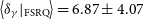
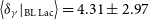
From our calculations, we obtained the average value of  $\gamma$
-ray Doppler factors for our whole sample,
$\gamma$
-ray Doppler factors for our whole sample,  $\langle\delta_{\gamma}\rangle|_{\textrm{blazar}}=5.39\pm3.70$
. For 342 FSRQs, we ascertain that their
$\langle\delta_{\gamma}\rangle|_{\textrm{blazar}}=5.39\pm3.70$
. For 342 FSRQs, we ascertain that their  $\gamma$
-ray Doppler factor, on average, is
$\gamma$
-ray Doppler factor, on average, is  $\langle\delta_{\gamma}\rangle|_{\textrm{FSRQ}}=6.87\pm4.07$
, ranging from
$\langle\delta_{\gamma}\rangle|_{\textrm{FSRQ}}=6.87\pm4.07$
, ranging from  $\delta_{\gamma}=1.04$
of J0625.8
$\delta_{\gamma}=1.04$
of J0625.8  $-$
5441 to
$-$
5441 to  $\delta_{\gamma}=28.38$
of J1833.6
$\delta_{\gamma}=28.38$
of J1833.6  $-$
2103. On the other hand, BL Lacs have the
$-$
2103. On the other hand, BL Lacs have the  $\gamma$
-ray Doppler factor, on average,
$\gamma$
-ray Doppler factor, on average,  $\langle\delta_{\gamma}|_{\textrm{BL\,Lac}}\rangle=4.31\pm2.97$
in the range from
$\langle\delta_{\gamma}|_{\textrm{BL\,Lac}}\rangle=4.31\pm2.97$
in the range from  $\delta_{\gamma}=0.95$
of J0113.7 + 0225 to
$\delta_{\gamma}=0.95$
of J0113.7 + 0225 to  $\delta_{\gamma}=22.81$
of J2055.4
$\delta_{\gamma}=22.81$
of J2055.4  $-$
0020. We present our sample and results in Table 1. In this table, Col. 1 gives 4FGL name; Col. 2 other name; Col. 3 classification (FSRQ, HBL, IBL, and LBL); Col. 4 redshift; Col. 5 core-dominance parameter; Col. 6 the X-ray flux density in units of
$-$
0020. We present our sample and results in Table 1. In this table, Col. 1 gives 4FGL name; Col. 2 other name; Col. 3 classification (FSRQ, HBL, IBL, and LBL); Col. 4 redshift; Col. 5 core-dominance parameter; Col. 6 the X-ray flux density in units of  $\mu$
Jy at 1 keV; Col. 7 X-ray spectral index; Col. 8 Reference for Col. 6 and 7; Col. 9
$\mu$
Jy at 1 keV; Col. 7 X-ray spectral index; Col. 8 Reference for Col. 6 and 7; Col. 9  $\gamma$
-ray photon index; Col. 10 average
$\gamma$
-ray photon index; Col. 10 average  $\gamma$
-ray photon energy in units of GeV; Col. 11 X-ray luminosity in units of erg
$\gamma$
-ray photon energy in units of GeV; Col. 11 X-ray luminosity in units of erg  $\text{s}^{-1}$
; Col. 12
$\text{s}^{-1}$
; Col. 12  $\gamma$
-ray luminosity in units of erg
$\gamma$
-ray luminosity in units of erg  $\text{s}^{-1}$
; Col. 13 the derived lower limit on
$\text{s}^{-1}$
; Col. 13 the derived lower limit on  $\gamma$
-ray Doppler factor in this paper; Col. 14 the estimated Doppler factor from Liodakis et al. (Reference Liodakis, Hovatta, Huppenkothen, Kiehlmann, Max-Moerbeck and Readhead2018); Col. 15 the estimated Doppler factor from Chen (Reference Chen2018). This table is available in its entirety in machine-readable form.
$\gamma$
-ray Doppler factor in this paper; Col. 14 the estimated Doppler factor from Liodakis et al. (Reference Liodakis, Hovatta, Huppenkothen, Kiehlmann, Max-Moerbeck and Readhead2018); Col. 15 the estimated Doppler factor from Chen (Reference Chen2018). This table is available in its entirety in machine-readable form.
The distributions of  $\delta_{\gamma}$
in logarithm for FSRQs and different classes of BL Lacs are shown in Figure 1. A Kolmogorov–Smirnov test (hereafter, K–S test) between the distributions of
$\delta_{\gamma}$
in logarithm for FSRQs and different classes of BL Lacs are shown in Figure 1. A Kolmogorov–Smirnov test (hereafter, K–S test) between the distributions of  $\delta_{\gamma}$
for FSRQs and BL Lacs shows that they belong to different parent distributions (
$\delta_{\gamma}$
for FSRQs and BL Lacs shows that they belong to different parent distributions ( $p=2.54\times10^{-27}$
). From the distributions and the K–S test result, we can find that
$p=2.54\times10^{-27}$
). From the distributions and the K–S test result, we can find that  $\langle \delta_{\gamma} \rangle|_{\textrm{FSRQ}}> \langle \delta_{\gamma} \rangle|_{\mathrm{BL\,Lac}}$
, indicating that the Fermi-detected FSRQs are more
$\langle \delta_{\gamma} \rangle|_{\textrm{FSRQ}}> \langle \delta_{\gamma} \rangle|_{\mathrm{BL\,Lac}}$
, indicating that the Fermi-detected FSRQs are more  $\gamma$
-ray Doppler-boosted.
$\gamma$
-ray Doppler-boosted.
Table 1. The lower limit on  $\gamma$
-ray Doppler factor for Fermi blazars
$\gamma$
-ray Doppler factor for Fermi blazars

Note: Col. 1 gives 4FGL name; Col. 2 counterpart name; Col. 3 classification (FSRQ: flat spectrum radio quasar; HBL: high synchrotron peak BL Lacs; IBL: intermediate synchrotron peak BL Lacs; LBL: low synchrotron peak BL Lacs); Col. 4 redshift; Col. 5 core-dominance parameter; Col. 6 the X-ray flux density in units of  $\mu$
Jy at 1 keV; Col. 7 X-ray spectral index; Col. 8 Reference for Col. 6 and 7 (Y19: Yang et al. (Reference Yang, Fan, Zhang, Yang, Tuo and Nie2019); NED: NASA/IPAC Extragalactic Database; BZCAT: The Roma BZCAT- 5th edition, Multi-frequency Catalogue of Blazars); Col. 9
$\mu$
Jy at 1 keV; Col. 7 X-ray spectral index; Col. 8 Reference for Col. 6 and 7 (Y19: Yang et al. (Reference Yang, Fan, Zhang, Yang, Tuo and Nie2019); NED: NASA/IPAC Extragalactic Database; BZCAT: The Roma BZCAT- 5th edition, Multi-frequency Catalogue of Blazars); Col. 9  $\gamma$
-ray photon index; Col. 10 average
$\gamma$
-ray photon index; Col. 10 average  $\gamma$
-ray photon energy in units of GeV; Col. 11 X-ray luminosity in units of erg s−1 Col. 12
$\gamma$
-ray photon energy in units of GeV; Col. 11 X-ray luminosity in units of erg s−1 Col. 12  $\gamma$
-ray luminosity in units of erg s−1; Col. 13 the derived lower limit on
$\gamma$
-ray luminosity in units of erg s−1; Col. 13 the derived lower limit on  $\gamma$
-ray Doppler factor; Col. 14 the estimated Doppler factor from Liodakis et al. (Reference Liodakis, Hovatta, Huppenkothen, Kiehlmann, Max-Moerbeck and Readhead2018); Col. 15 the estimated Doppler factor from Chen (Reference Chen2018). (The table is available in its entirety in machine-readable form)
$\gamma$
-ray Doppler factor; Col. 14 the estimated Doppler factor from Liodakis et al. (Reference Liodakis, Hovatta, Huppenkothen, Kiehlmann, Max-Moerbeck and Readhead2018); Col. 15 the estimated Doppler factor from Chen (Reference Chen2018). (The table is available in its entirety in machine-readable form)

Figure 1. Distributions of the lower limit on  $\gamma$
-ray Doppler factor (
$\gamma$
-ray Doppler factor ( $\delta_{\gamma}$
) in logarithm for all subclasses.
$\delta_{\gamma}$
) in logarithm for all subclasses.
4. Discussion
Blazars, as the subclass of AGNs, show extreme observational properties, which are associated with the relativistic beaming effect. All of these extreme properties indicate that blazars are the most active extragalactic sources in the universe. BL Lac objects are usually identified as ‘lineless’ AGNs and conversely, quasars show strong broad emission lines. The core-dominance parameter, R, can be used for the orientation indicator of the jet (Urry & Padovani Reference Urry and Padovani1995). Since the Doppler factor is not observable and cannot be determined accurately, thus the core-dominance parameter might be an eligible indicator of Doppler beaming effect.
As ever, blazars take a majority of sources detected by Fermi (Abdo et al. Reference Abdo2009, Reference Abdo2010a,d; Acero et al. Reference Acero2015). Pei et al. (Reference Pei, Fan, Bastieri, Yang and Xiao2020b) present a up-to-date largest catalogue of available core-dominance parameters R. We point out that R are quite different for diverse subclasses of AGNs, and particularly, Fermi blazars hold, on average, higher R than the non- Fermi blazars, indicating that the  $\gamma$
-emissions of Fermi blazars are from the jet and more Doppler-boosted. The
$\gamma$
-emissions of Fermi blazars are from the jet and more Doppler-boosted. The  $\gamma$
-emission is strongly beamed (Fan et al. Reference Fan, Huang, He, Yang, Hua, Liu and Wang2009; Pei et al. Reference Pei2016, Reference Pei, Fan, Bastieri, Yang and Xiao2020b).
$\gamma$
-emission is strongly beamed (Fan et al. Reference Fan, Huang, He, Yang, Hua, Liu and Wang2009; Pei et al. Reference Pei2016, Reference Pei, Fan, Bastieri, Yang and Xiao2020b).

Figure 2. Plot of the correlation between  $\log \delta_{\gamma}$
derived in this paper and that presented from other literature after cross-checking.
$\log \delta_{\gamma}$
derived in this paper and that presented from other literature after cross-checking.  $\log \delta_{\textrm{L18}}$
denotes the variability Doppler factor adopted from Liodakis et al. (Reference Liodakis, Hovatta, Huppenkothen, Kiehlmann, Max-Moerbeck and Readhead2018) (left panel) and
$\log \delta_{\textrm{L18}}$
denotes the variability Doppler factor adopted from Liodakis et al. (Reference Liodakis, Hovatta, Huppenkothen, Kiehlmann, Max-Moerbeck and Readhead2018) (left panel) and  $\log \delta_{\textrm{C18}}$
denotes the SED fitting derived Doppler factor from Chen (Reference Chen2018) (right panel). The solid blue lines refer to the equality line and the dashed pink ones signify the half proportion dividing line that are parallel to the equality one.
$\log \delta_{\textrm{C18}}$
denotes the SED fitting derived Doppler factor from Chen (Reference Chen2018) (right panel). The solid blue lines refer to the equality line and the dashed pink ones signify the half proportion dividing line that are parallel to the equality one.
The strongly Doppler-boosted emission is referable to the relativistic beaming effect which enhances the observed flux density by a factor of  $\delta^{2+\alpha}$
for stationery and continuous jet, and
$\delta^{2+\alpha}$
for stationery and continuous jet, and  $\delta^{3+\alpha}$
for a moving blob. Since the
$\delta^{3+\alpha}$
for a moving blob. Since the  $\gamma$
-ray blazars are transparent to
$\gamma$
-ray blazars are transparent to  $\gamma\gamma$
pair production within a small region deducted from the fast
$\gamma\gamma$
pair production within a small region deducted from the fast  $\gamma$
-ray variability, strongly suggesting that the
$\gamma$
-ray variability, strongly suggesting that the  $\gamma$
-ray emission produced from the jets of blazars is also Doppler-beamed, which is similar to the behaviour of radio emission (von Montigny et al. Reference von Montigny1995; Mattox et al. Reference Mattox1993; Fan et al. Reference Fan, Huang, He, Yang, Hua, Liu and Wang2009). Therefore, the estimation of
$\gamma$
-ray emission produced from the jets of blazars is also Doppler-beamed, which is similar to the behaviour of radio emission (von Montigny et al. Reference von Montigny1995; Mattox et al. Reference Mattox1993; Fan et al. Reference Fan, Huang, He, Yang, Hua, Liu and Wang2009). Therefore, the estimation of  $\gamma$
-ray Doppler factor is reasonable and substantial to explore the typical characteristic of
$\gamma$
-ray Doppler factor is reasonable and substantial to explore the typical characteristic of  $\gamma$
-ray loud blazars and beaming effect (Fan et al. Reference Fan, Yang, Liu and Zhang2013a, Reference Fan, Bastieri, Yang, Liu, Hua, Yuan and Wu2014).
$\gamma$
-ray loud blazars and beaming effect (Fan et al. Reference Fan, Yang, Liu and Zhang2013a, Reference Fan, Bastieri, Yang, Liu, Hua, Yuan and Wu2014).
4.1. Comparison with other Doppler factors in the literature
The Doppler factor ( $\delta$
), an important parameter to reveal the relativistic beaming effect and explain the observed extreme properties of blazars, is proverbially unmanageable to measure since there is no straight method at present. Many indirect methods are proposed to estimate the beaming Doppler factor: (i) it can be deduced by a synchrotron self-Compton (SSC) model thus denoted as
$\delta$
), an important parameter to reveal the relativistic beaming effect and explain the observed extreme properties of blazars, is proverbially unmanageable to measure since there is no straight method at present. Many indirect methods are proposed to estimate the beaming Doppler factor: (i) it can be deduced by a synchrotron self-Compton (SSC) model thus denoted as  $\delta_{\textrm{ssc}}$
(e.g. Ghisellini et al. Reference Ghisellini, Padovani, Celotti and Maraschi1993); (ii) to be derived from adopting single-epoch radio data by assuming that the sources hold an equipartition of energy between radiating particles and magnetic field as denoted as
$\delta_{\textrm{ssc}}$
(e.g. Ghisellini et al. Reference Ghisellini, Padovani, Celotti and Maraschi1993); (ii) to be derived from adopting single-epoch radio data by assuming that the sources hold an equipartition of energy between radiating particles and magnetic field as denoted as  $\delta_{\textrm{eq}}$
(Readhead Reference Readhead1994); (iii) to be estimated using the radio flux density variations or brightness temperature denoted as
$\delta_{\textrm{eq}}$
(Readhead Reference Readhead1994); (iii) to be estimated using the radio flux density variations or brightness temperature denoted as  $\delta_{\textrm{var}}$
(Lähteenmäki & Valtaoja Reference Lähteenmäki and Valtaoja1999; Hovatta et al. Reference Hovatta, Valtaoja, Tornikoski and Lähteenmäki2009). (iv) One can calculate it based on the broadband SED (e.g. Chen Reference Chen2018). However, due to these different assumptions, each method will render discrepant results.
$\delta_{\textrm{var}}$
(Lähteenmäki & Valtaoja Reference Lähteenmäki and Valtaoja1999; Hovatta et al. Reference Hovatta, Valtaoja, Tornikoski and Lähteenmäki2009). (iv) One can calculate it based on the broadband SED (e.g. Chen Reference Chen2018). However, due to these different assumptions, each method will render discrepant results.
The relativistic beaming effect plays a crucial role in the  $\gamma$
-ray emission, and particularly, for Fermi-detected blazars. Fan et al. (Reference Fan, Huang, He, Yang, Hua, Liu and Wang2009) found that the
$\gamma$
-ray emission, and particularly, for Fermi-detected blazars. Fan et al. (Reference Fan, Huang, He, Yang, Hua, Liu and Wang2009) found that the  $\gamma$
-ray luminosity of Fermi-detected blazars correlates tightly with the radio Doppler factor
$\gamma$
-ray luminosity of Fermi-detected blazars correlates tightly with the radio Doppler factor  $\log L_{\gamma} \sim 0.47\log \delta^{3+\alpha}_{\textrm{R}}$
. Kovalev (Reference Kovalev2009) pointed out that the sources detected by Fermi/LAT have higher brightness temperature with respect to those not detected by Fermi. Savolainen et al. (Reference Savolainen2010) compiled 62 AGNs with apparent superluminal motion and adopted their Doppler factors from Hovatta et al. (Reference Hovatta, Valtaoja, Tornikoski and Lähteenmäki2009) and found that the Fermi blazars have, on average, higher Doppler factor than non- Fermi-detected blazars. Xiao et al. (Reference Xiao2019) collected 291 sources with superluminal motions, in which 189 are
$\log L_{\gamma} \sim 0.47\log \delta^{3+\alpha}_{\textrm{R}}$
. Kovalev (Reference Kovalev2009) pointed out that the sources detected by Fermi/LAT have higher brightness temperature with respect to those not detected by Fermi. Savolainen et al. (Reference Savolainen2010) compiled 62 AGNs with apparent superluminal motion and adopted their Doppler factors from Hovatta et al. (Reference Hovatta, Valtaoja, Tornikoski and Lähteenmäki2009) and found that the Fermi blazars have, on average, higher Doppler factor than non- Fermi-detected blazars. Xiao et al. (Reference Xiao2019) collected 291 sources with superluminal motions, in which 189 are  $\gamma$
-ray sources detected by Fermi, and reported that the Fermi-detected sources show higher proper motion, apparent velocity, Doppler factor, Lorentz factor, and smaller viewing angles than non- Fermi-detected sources, also suggesting the strong Doppler effect lies on those
$\gamma$
-ray sources detected by Fermi, and reported that the Fermi-detected sources show higher proper motion, apparent velocity, Doppler factor, Lorentz factor, and smaller viewing angles than non- Fermi-detected sources, also suggesting the strong Doppler effect lies on those  $\gamma$
-ray sources. Pei et al. (Reference Pei, Fan, Bastieri, Yang and Xiao2020b) obtained that the
$\gamma$
-ray sources. Pei et al. (Reference Pei, Fan, Bastieri, Yang and Xiao2020b) obtained that the  $\gamma$
-ray luminosity increases with radio core-dominance parameter for Fermi AGNs.
$\gamma$
-ray luminosity increases with radio core-dominance parameter for Fermi AGNs.
Beaming effect is mostly studied using the radio emission, which yields that the radio variability Doppler factor ( $\delta_{\textrm{var}}$
) method should be perhaps an appropriate way to describe the blazars population and beaming effect (Fan et al. Reference Fan, Huang, He, Yang, Hua, Liu and Wang2009, Reference Fan, Yang, Zhang, Hua, Liu, Qin and Huang2013b; Liodakis & Pavlidou Reference Liodakis and Pavlidou2015; Liodakis et al. Reference Liodakis2017a,b).
$\delta_{\textrm{var}}$
) method should be perhaps an appropriate way to describe the blazars population and beaming effect (Fan et al. Reference Fan, Huang, He, Yang, Hua, Liu and Wang2009, Reference Fan, Yang, Zhang, Hua, Liu, Qin and Huang2013b; Liodakis & Pavlidou Reference Liodakis and Pavlidou2015; Liodakis et al. Reference Liodakis2017a,b).
By modelling the radio light curves of 1 029 sources as a series of flares characterised by an exponential rise and decay, Liodakis et al. (Reference Liodakis, Hovatta, Huppenkothen, Kiehlmann, Max-Moerbeck and Readhead2018) estimated the variability Doppler factor ( $\delta_{\textrm{var}}$
) for 837 blazars, which included 670 FSRQs and 167 BL Lacs. They calculated the variability brightness temperature (
$\delta_{\textrm{var}}$
) for 837 blazars, which included 670 FSRQs and 167 BL Lacs. They calculated the variability brightness temperature ( $T_{\textrm{var}}$
) using
$T_{\textrm{var}}$
) using
 \begin{equation}T_{\textrm{var}} = 1.47\times10^{13}\displaystyle\frac{d^{2}_{\textrm{L}}\Delta S_{\textrm{ob}}(\nu)}{\nu^{2}t^{2}_{\textrm{var}}(1+z)^{4}}{\rm K},\end{equation}
here,  $S_{\textrm{ob}}(\nu)$
the amplitude of the flare in Jy,
$S_{\textrm{ob}}(\nu)$
the amplitude of the flare in Jy,  $\nu$
the observed frequency in GHz, and
$\nu$
the observed frequency in GHz, and  $t_{\textrm{var}}$
the rise time of a flare in days. Then, the variability Doppler factor (
$t_{\textrm{var}}$
the rise time of a flare in days. Then, the variability Doppler factor ( $\delta_{\textrm{var}}$
) can be defined as:
$\delta_{\textrm{var}}$
) can be defined as:
 \begin{equation}\delta_{\textrm{var}}=(1+z)\sqrt[3]{\frac{T_{\textrm{var}}}{T_{\textrm{eq}}}},\end{equation}
where  $T_{\textrm{eq}}$
is the equipartition brightness temperature, and
$T_{\textrm{eq}}$
is the equipartition brightness temperature, and  $T_{\textrm{eq}}=2.78\times10^{11}$
K was adopted. After cross-checking with our sample, there are 285 common sources, which contains 210 FSRQs and 75 BL Lacs. When we compared our results with theirs, it was found that
$T_{\textrm{eq}}=2.78\times10^{11}$
K was adopted. After cross-checking with our sample, there are 285 common sources, which contains 210 FSRQs and 75 BL Lacs. When we compared our results with theirs, it was found that  $\log \delta_{\gamma}=(0.22\pm0.03)\log \delta_{\textrm{L18}}+(0.49\pm0.04)$
with a correlation coefficient
$\log \delta_{\gamma}=(0.22\pm0.03)\log \delta_{\textrm{L18}}+(0.49\pm0.04)$
with a correlation coefficient  $r=0.37$
and a chance probability of
$r=0.37$
and a chance probability of  $P<10^{-10}$
. We show this plot in the left panel of Figure 2.
$P<10^{-10}$
. We show this plot in the left panel of Figure 2.
Based on the SED fitting, Chen (Reference Chen2018) estimated the jet physical parameters of 1 392  $\gamma$
-ray loud blazars taking from Fan et al. (Reference Fan2016), and particularly, they calculated the Doppler factor (
$\gamma$
-ray loud blazars taking from Fan et al. (Reference Fan2016), and particularly, they calculated the Doppler factor ( $\delta_{\textrm{SED}}$
) and obtained that the median values of the Doppler factors of FSRQs, BL Lacs, and total blazars were 10.7, 22.3, and 13.1, respectively. It is usually assumed in SED modelling that the
$\delta_{\textrm{SED}}$
) and obtained that the median values of the Doppler factors of FSRQs, BL Lacs, and total blazars were 10.7, 22.3, and 13.1, respectively. It is usually assumed in SED modelling that the  $\gamma$
-ray emission is produced closer to the supermassive black hole than the radio core of the jet where most of the radio emission originates. For comparison, we investigate the relation between the derived
$\gamma$
-ray emission is produced closer to the supermassive black hole than the radio core of the jet where most of the radio emission originates. For comparison, we investigate the relation between the derived  $\delta_{\gamma}$
in the present paper and those in Chen (Reference Chen2018) for 597 sources are in common in both papers (in fact, we found 682 sources to be in common after cross-checking; however, there are 85 sources obtained an extremely large or small value of
$\delta_{\gamma}$
in the present paper and those in Chen (Reference Chen2018) for 597 sources are in common in both papers (in fact, we found 682 sources to be in common after cross-checking; however, there are 85 sources obtained an extremely large or small value of  $\delta_{\textrm{SED}}$
in Chen (Reference Chen2018), thus we excluded those 85 sources). The best fitting is
$\delta_{\textrm{SED}}$
in Chen (Reference Chen2018), thus we excluded those 85 sources). The best fitting is  $\log \delta_{\gamma}=(0.21\pm0.02)\log \delta_{\textrm{C18}}+(0.45\pm0.03)$
with
$\log \delta_{\gamma}=(0.21\pm0.02)\log \delta_{\textrm{C18}}+(0.45\pm0.03)$
with  $r=0.34$
and
$r=0.34$
and  $P\sim0$
for the 597 sources (see the right panel of Figure 2).
$P\sim0$
for the 597 sources (see the right panel of Figure 2).
However, according to equation (5), the estimation of lower limit on  $\delta_{\gamma}$
would be affected by redshift, the above correlations then have a redshift dependence, thus the redshift effect needs to be removed. To do so, we adopt a partial correlation analysis (see e.g. Padovani Reference Padovani1992):
$\delta_{\gamma}$
would be affected by redshift, the above correlations then have a redshift dependence, thus the redshift effect needs to be removed. To do so, we adopt a partial correlation analysis (see e.g. Padovani Reference Padovani1992):
 \begin{equation}r_{12,3} = \displaystyle\frac{r_{12}-r_{13}r_{23}}{\sqrt{1-r^{2}_{13}}\sqrt{1-r^{2}_{23}}},\end{equation}
where  $r_{ij}$
denotes the correlation coefficient between
$r_{ij}$
denotes the correlation coefficient between  $x_{i}$
and
$x_{i}$
and  $x_{j}$
, while
$x_{j}$
, while  $r_{ij,k}$
denotes the partial correlation coefficient between
$r_{ij,k}$
denotes the partial correlation coefficient between  $x_{i}$
and
$x_{i}$
and  $x_{j}$
with
$x_{j}$
with  $x_{k}$
dependence excluded (
$x_{k}$
dependence excluded ( $i, j, k=1,2,3$
). In our case, we let
$i, j, k=1,2,3$
). In our case, we let  $x_{1}=\log\delta_{\gamma}$
,
$x_{1}=\log\delta_{\gamma}$
,  $x_{2}=\log\delta_{\textrm{L18}}$
or
$x_{2}=\log\delta_{\textrm{L18}}$
or  $\log\delta_{\textrm{C18}}$
, and
$\log\delta_{\textrm{C18}}$
, and  $x_{3}=z$
. For the left panel, we have
$x_{3}=z$
. For the left panel, we have  $r_{12}=0.37$
,
$r_{12}=0.37$
,  $r_{1z}=0.74$
, and
$r_{1z}=0.74$
, and  $r_{2z}=0.31$
, which yields
$r_{2z}=0.31$
, which yields  $r_{12,z}=0.21$
. Using the similar calculation, we obtain
$r_{12,z}=0.21$
. Using the similar calculation, we obtain  $r_{12,z}=0.19$
for the right panel. Their P-values are both
$r_{12,z}=0.19$
for the right panel. Their P-values are both  $<10^{-4}$
. It still rendered a statistically correlation between our derived values of
$<10^{-4}$
. It still rendered a statistically correlation between our derived values of  $\log\delta_{\gamma}$
and those from other methods after removing the redshift effect, implying that they are truly correlated. This result indicates that our derived lower limit on
$\log\delta_{\gamma}$
and those from other methods after removing the redshift effect, implying that they are truly correlated. This result indicates that our derived lower limit on  $\gamma$
-ray Doppler factors are reasonable.
$\gamma$
-ray Doppler factors are reasonable.
We draw an equality line in both panels of Figure 2 (labelled in blue solid) and note that some points are quite disperse and most importantly, the derived values of  $\log \delta_{\gamma}$
are fairly small than that of
$\log \delta_{\gamma}$
are fairly small than that of  $\log \delta_{\textrm{var}}$
or
$\log \delta_{\textrm{var}}$
or  $\log \delta_{\textrm{SED}}$
and the range is relatively compact, ranging from 0.95 to 28.38 and the average value is 5.39. We should point out that, firstly, because our estimation is the lower limit on
$\log \delta_{\textrm{SED}}$
and the range is relatively compact, ranging from 0.95 to 28.38 and the average value is 5.39. We should point out that, firstly, because our estimation is the lower limit on  $\delta_{\gamma}$
. Hovatta et al. (Reference Hovatta, Valtaoja, Tornikoski and Lähteenmäki2009) had shown the median value of
$\delta_{\gamma}$
. Hovatta et al. (Reference Hovatta, Valtaoja, Tornikoski and Lähteenmäki2009) had shown the median value of  $\delta$
was 12.02 ranging from 0.30 to 35.50; Liodakis et al. (Reference Liodakis, Hovatta, Huppenkothen, Kiehlmann, Max-Moerbeck and Readhead2018) reported the average value to be 14.35 in the range from 0.08 to 88.44; Chen (Reference Chen2018) on average, 14.30 was obtained and spanning from 1.00 to 99.50. The typical values of Doppler factor in blazars should be in the range from a few to
$\delta$
was 12.02 ranging from 0.30 to 35.50; Liodakis et al. (Reference Liodakis, Hovatta, Huppenkothen, Kiehlmann, Max-Moerbeck and Readhead2018) reported the average value to be 14.35 in the range from 0.08 to 88.44; Chen (Reference Chen2018) on average, 14.30 was obtained and spanning from 1.00 to 99.50. The typical values of Doppler factor in blazars should be in the range from a few to  ${\sim}$
50 based on various methods as mentioned above. However, since our derived results are the lower limit on
${\sim}$
50 based on various methods as mentioned above. However, since our derived results are the lower limit on  $\delta_{\gamma}$
, thus the distribution of
$\delta_{\gamma}$
, thus the distribution of  $\delta_{\gamma}$
should be smaller than those from the literature. This is consistent with Dondi & Ghisellini (Reference Dondi and Ghisellini1995), they found the average value
$\delta_{\gamma}$
should be smaller than those from the literature. This is consistent with Dondi & Ghisellini (Reference Dondi and Ghisellini1995), they found the average value  $\langle\delta_{\gamma}\rangle\sim4.4$
, ranging from 1.3 to 11 for a sample of EGRET blazars. Fan et al. (Reference Fan, Yang, Liu and Zhang2013a) obtained an average value
$\langle\delta_{\gamma}\rangle\sim4.4$
, ranging from 1.3 to 11 for a sample of EGRET blazars. Fan et al. (Reference Fan, Yang, Liu and Zhang2013a) obtained an average value  $\langle\delta_{\gamma}\rangle\sim7.22$
for 138
$\langle\delta_{\gamma}\rangle\sim7.22$
for 138  $\gamma$
-ray blazars and Fan et al. (Reference Fan, Bastieri, Yang, Liu, Hua, Yuan and Wu2014) also found the average value was
$\gamma$
-ray blazars and Fan et al. (Reference Fan, Bastieri, Yang, Liu, Hua, Yuan and Wu2014) also found the average value was  ${\sim}$
7.00 with regard to their sample.
${\sim}$
7.00 with regard to their sample.
Secondly, since we could not ascertain the variability timescale for each source in our large sample, thus we adopted  $\Delta T=24$
h (1 d) in our present calculation. However, this operation was examined by Fan et al. (Reference Fan, Yang, Liu and Zhang2013a) and Fan et al. (Reference Fan, Bastieri, Yang, Liu, Hua, Yuan and Wu2014), who also used
$\Delta T=24$
h (1 d) in our present calculation. However, this operation was examined by Fan et al. (Reference Fan, Yang, Liu and Zhang2013a) and Fan et al. (Reference Fan, Bastieri, Yang, Liu, Hua, Yuan and Wu2014), who also used  $\Delta T=1$
d for calculation and obtained reliable results. For instance, those authors found a tendency for the
$\Delta T=1$
d for calculation and obtained reliable results. For instance, those authors found a tendency for the  $\gamma$
-ray Doppler factors to increase with the radio Doppler factors and
$\gamma$
-ray Doppler factors to increase with the radio Doppler factors and  $\delta_{\gamma}$
are also correlated with the superluminal velocity. This supports the fact that the
$\delta_{\gamma}$
are also correlated with the superluminal velocity. This supports the fact that the  $\gamma$
-rays are strongly beamed, and likewise suggesting that the radio Doppler factors estimated from the variability can be used to discuss the beaming effect in Fermi loud blazars. Dondi & Ghisellini (Reference Dondi and Ghisellini1995) used a similar method as this paper to estimate the lower limit on
$\gamma$
-rays are strongly beamed, and likewise suggesting that the radio Doppler factors estimated from the variability can be used to discuss the beaming effect in Fermi loud blazars. Dondi & Ghisellini (Reference Dondi and Ghisellini1995) used a similar method as this paper to estimate the lower limit on  $\delta_{\gamma}$
for 46
$\delta_{\gamma}$
for 46  $\gamma$
-ray loud blazars. They could not find enough information of variability timescale for nearly half of their sample either, and they also adopted
$\gamma$
-ray loud blazars. They could not find enough information of variability timescale for nearly half of their sample either, and they also adopted  $\Delta T=1$
d for calculation. However, different synchrotron peaked sources may have different timescales. Abdo et al. (Reference Abdo2011), Bonnoli et al. (Reference Bonnoli, Ghisellini, Foschini, Tavecchio and Ghirlanda2011), Hu et al. (Reference Hu, Chen, Guo, Jiang and Li2014), and Prince (Reference Prince2020) processed systematic well studied on Mrk 421, 3C 454.3, S5 0716 + 714, and 3C279, respectively, although Mrk 421 is a HSP blazar and the other three are LSP blazars (Fan et al. Reference Fan2016), those authors had shown that a typical variability timescale in the source frame for Fermi/LAT blazars is
$\Delta T=1$
d for calculation. However, different synchrotron peaked sources may have different timescales. Abdo et al. (Reference Abdo2011), Bonnoli et al. (Reference Bonnoli, Ghisellini, Foschini, Tavecchio and Ghirlanda2011), Hu et al. (Reference Hu, Chen, Guo, Jiang and Li2014), and Prince (Reference Prince2020) processed systematic well studied on Mrk 421, 3C 454.3, S5 0716 + 714, and 3C279, respectively, although Mrk 421 is a HSP blazar and the other three are LSP blazars (Fan et al. Reference Fan2016), those authors had shown that a typical variability timescale in the source frame for Fermi/LAT blazars is  $\approx$
1 d (see also Nalewajko Reference Nalewajko2013; Zhang et al. Reference Zhang, Xue, He, Liang and Zhang2015). Chen (Reference Chen2018) also adopted this idea for simplicity in the constraint of Doppler factor from SED modelling for a larger sample of blazars (see also Kang, Chen, & Wu Reference Kang, Chen and Wu2014). From this point of view, we consider that our choice of variability timescale that
$\approx$
1 d (see also Nalewajko Reference Nalewajko2013; Zhang et al. Reference Zhang, Xue, He, Liang and Zhang2015). Chen (Reference Chen2018) also adopted this idea for simplicity in the constraint of Doppler factor from SED modelling for a larger sample of blazars (see also Kang, Chen, & Wu Reference Kang, Chen and Wu2014). From this point of view, we consider that our choice of variability timescale that  $\Delta T=1$
d is also reliable.
$\Delta T=1$
d is also reliable.
On the other hand, therefore, different values of  $\Delta T$
can be also considered. We compute the
$\Delta T$
can be also considered. We compute the  $\gamma$
-ray Doppler factor with
$\gamma$
-ray Doppler factor with  $\Delta T=6$
h (denoted in
$\Delta T=6$
h (denoted in  $\delta_{\gamma}^{\rm6\,h}$
) and
$\delta_{\gamma}^{\rm6\,h}$
) and  $\Delta T=48$
h (denoted in
$\Delta T=48$
h (denoted in  $\delta_{\gamma}^{\rm48\,h}$
), then a relation is found
$\delta_{\gamma}^{\rm48\,h}$
), then a relation is found  $\delta_{\gamma}^{\rm6\,h}\sim1.32\delta_{\gamma}^{\rm24\,h}$
and
$\delta_{\gamma}^{\rm6\,h}\sim1.32\delta_{\gamma}^{\rm24\,h}$
and  $\delta_{\gamma}^{\rm48\,h}\sim0.87\delta_{\gamma}^{\rm24\,h}$
. A slight higher than our present result if we choose
$\delta_{\gamma}^{\rm48\,h}\sim0.87\delta_{\gamma}^{\rm24\,h}$
. A slight higher than our present result if we choose  $\Delta T=6$
h and smaller while
$\Delta T=6$
h and smaller while  $\Delta T=48$
h is considered (see also Fan et al. Reference Fan, Bastieri, Yang, Liu, Hua, Yuan and Wu2014). For the sake of simplicity, we adopt
$\Delta T=48$
h is considered (see also Fan et al. Reference Fan, Bastieri, Yang, Liu, Hua, Yuan and Wu2014). For the sake of simplicity, we adopt  $\Delta T=24$
h in this paper for calculation as did in Dondi & Ghisellini (Reference Dondi and Ghisellini1995), Fan et al. (Reference Fan, Yang, Liu and Zhang2013a), and Fan et al. (Reference Fan, Bastieri, Yang, Liu, Hua, Yuan and Wu2014). Besides, the non-simultaneous observations will also result in some discrepancies.
$\Delta T=24$
h in this paper for calculation as did in Dondi & Ghisellini (Reference Dondi and Ghisellini1995), Fan et al. (Reference Fan, Yang, Liu and Zhang2013a), and Fan et al. (Reference Fan, Bastieri, Yang, Liu, Hua, Yuan and Wu2014). Besides, the non-simultaneous observations will also result in some discrepancies.
For comparison, we draw a half proportion dividing line that is parallel to the equality line in two panel (labelled in dashed pink), which means there are 50/50 distribution of sources on two sides. When we consider this line in the plot of  $\log \delta_{\gamma}$
versus
$\log \delta_{\gamma}$
versus  $\log \delta_{\textrm{L18}}$
, it corresponds to a variability timescale
$\log \delta_{\textrm{L18}}$
, it corresponds to a variability timescale  $\Delta T \sim$
2 h. For the case of
$\Delta T \sim$
2 h. For the case of  $\log \delta_{\gamma}$
versus
$\log \delta_{\gamma}$
versus  $\log \delta_{\textrm{C18}}$
, we found
$\log \delta_{\textrm{C18}}$
, we found  $\Delta T \sim$
1.5 h. This could suggest that the on average, variability timescale for Fermi-detected blazars is around 1.5
$\Delta T \sim$
1.5 h. This could suggest that the on average, variability timescale for Fermi-detected blazars is around 1.5 $\,\sim\,$
2 h; however, we cannot reach firm conclusions.
$\,\sim\,$
2 h; however, we cannot reach firm conclusions.
Based on the SSC limit, a so-called ‘classical’ method to estimate the Doppler factor, Ghisellini et al. (Reference Ghisellini, Padovani, Celotti and Maraschi1993) constrained a relation between the  $\delta$
derived from moving sphere and a continuous jet:
$\delta$
derived from moving sphere and a continuous jet:
 \begin{equation}\delta_{3+\alpha}^{(4+2\alpha)/(3+2\alpha)}=\delta_{2+\alpha}.\end{equation}
We also assume that the emission region from the jet is spherical, which means  $p=3+\alpha$
has been taken into account. Note that, if the source is a continuous jet,
$p=3+\alpha$
has been taken into account. Note that, if the source is a continuous jet,  $p=2+\alpha$
, then the equation (5) of derived
$p=2+\alpha$
, then the equation (5) of derived  $\delta_{\gamma}$
should be regenerated as:
$\delta_{\gamma}$
should be regenerated as:
 \begin{equation}\begin{aligned}\delta_{\gamma}\ge\left[{1.54\times10^{-3}\displaystyle\left(1+z\right)^{3+2\alpha}\left(\frac{d_{L}}{\rm Mpc}\right)^{2}\left(\frac{\Delta T}{\rm h}\right)^{-1}} \right. \\\left. \left(\frac{F_{\textrm{1\,keV}}}{\mu \rm Jy}\right){\left(\frac{E_{\gamma}}{\rm GeV}\right)^{\alpha}}\right]^{\frac{1}{3+2\alpha}}.\end{aligned}\end{equation}
For comparison, we also estimate the lower limit on  $\gamma$
-ray Doppler factor for this case and obtain
$\gamma$
-ray Doppler factor for this case and obtain  $\langle\delta_{\gamma}|_{\textrm{FSRQ}}\rangle=8.93\pm6.78$
and
$\langle\delta_{\gamma}|_{\textrm{FSRQ}}\rangle=8.93\pm6.78$
and  $\langle\delta_{\gamma}|_{\textrm{BL\,Lac}}\rangle=5.42\pm4.29$
with P-value of K–S test indicating the two distributions being from the same apparent distribution is
$\langle\delta_{\gamma}|_{\textrm{BL\,Lac}}\rangle=5.42\pm4.29$
with P-value of K–S test indicating the two distributions being from the same apparent distribution is  $P=4.58\times10^{-35}$
. Our results show that
$P=4.58\times10^{-35}$
. Our results show that  $\log\delta_{\gamma}^{2+\alpha}\sim1.14\log\delta_{\gamma}^{3+\alpha}$
for FSRQs and
$\log\delta_{\gamma}^{2+\alpha}\sim1.14\log\delta_{\gamma}^{3+\alpha}$
for FSRQs and  $\log\delta_{\gamma}^{2+\alpha}\sim1.13\log\delta_{\gamma}^{3+\alpha}$
for BL Lacs. We can find the estimated value of
$\log\delta_{\gamma}^{2+\alpha}\sim1.13\log\delta_{\gamma}^{3+\alpha}$
for BL Lacs. We can find the estimated value of  $\delta_{\gamma}$
for the case of continuous jet to be larger than that of moving blob sphere, and FSRQs also have on average higher
$\delta_{\gamma}$
for the case of continuous jet to be larger than that of moving blob sphere, and FSRQs also have on average higher  $\gamma$
-ray Doppler factor than BL Lacs.
$\gamma$
-ray Doppler factor than BL Lacs.
From our calculation, FSRQs have on average significantly higher  $\delta_{\gamma}$
than BL Lacs (P-value is
$\delta_{\gamma}$
than BL Lacs (P-value is  $2.54\times10^{-27}$
from K–S test), which is consistent with estimations from other literatures (Fan et al. Reference Fan, Huang, He, Yang, Hua, Liu and Wang2009; Hovatta et al. Reference Hovatta, Valtaoja, Tornikoski and Lähteenmäki2009; Fan et al. Reference Fan, Yang, Liu and Zhang2013a, Reference Fan, Bastieri, Yang, Liu, Hua, Yuan and Wu2014; Liodakis et al. Reference Liodakis, Hovatta, Huppenkothen, Kiehlmann, Max-Moerbeck and Readhead2018). In the standard model of AGNs, FSRQs should have a smaller viewing angle
$2.54\times10^{-27}$
from K–S test), which is consistent with estimations from other literatures (Fan et al. Reference Fan, Huang, He, Yang, Hua, Liu and Wang2009; Hovatta et al. Reference Hovatta, Valtaoja, Tornikoski and Lähteenmäki2009; Fan et al. Reference Fan, Yang, Liu and Zhang2013a, Reference Fan, Bastieri, Yang, Liu, Hua, Yuan and Wu2014; Liodakis et al. Reference Liodakis, Hovatta, Huppenkothen, Kiehlmann, Max-Moerbeck and Readhead2018). In the standard model of AGNs, FSRQs should have a smaller viewing angle  $\theta$
with regard to BL Lacs, thus showing stronger Doppler-boosted effect and resulting in a larger
$\theta$
with regard to BL Lacs, thus showing stronger Doppler-boosted effect and resulting in a larger  $\delta$
due to the definition of Doppler factor
$\delta$
due to the definition of Doppler factor  $\delta=[\Gamma(1-\beta\cos\theta)]^{-1}$
. In the cross-checked sample with Liodakis et al. (Reference Liodakis, Hovatta, Huppenkothen, Kiehlmann, Max-Moerbeck and Readhead2018), 157 out of 285 sources were given the estimation of viewing angle, which included 127 FSRQs with average around
$\delta=[\Gamma(1-\beta\cos\theta)]^{-1}$
. In the cross-checked sample with Liodakis et al. (Reference Liodakis, Hovatta, Huppenkothen, Kiehlmann, Max-Moerbeck and Readhead2018), 157 out of 285 sources were given the estimation of viewing angle, which included 127 FSRQs with average around  $\langle\theta\rangle|_{\textrm{FSRQ}}\sim4.61$
deg and 30 BL Lacs with
$\langle\theta\rangle|_{\textrm{FSRQ}}\sim4.61$
deg and 30 BL Lacs with  $\langle\theta\rangle|_{\textrm{BL\,Lac}}\sim10.20$
deg, leading FSRQs have higher
$\langle\theta\rangle|_{\textrm{BL\,Lac}}\sim10.20$
deg, leading FSRQs have higher  $\delta$
than BL Lacs.
$\delta$
than BL Lacs.
As for the weaker emission line features in BL Lacs is mainly ascribable to the fact that the isotropic emission component in BL Lacs is intrinsically weaker than in FSRQs and directs to different parent populations for the two subclasses of blazars (Madau, Ghisellini, & Persic Reference Madau, Ghisellini and Persic1987; Ghisellini et al. Reference Ghisellini, Padovani, Celotti and Maraschi1993). For example, Padovani (Reference Padovani1992) pointed out that [O  $III$
] line luminosity and radio-extended luminosity for BL Lacs are lower than for FSRQs with two orders of magnitude. It is possible that the different emission line property is from the factor that the ratio of the core emission to the extend one in the co-moving frame is higher in BL Lacs than in FSRQs (Fan Reference Fan2003).
$III$
] line luminosity and radio-extended luminosity for BL Lacs are lower than for FSRQs with two orders of magnitude. It is possible that the different emission line property is from the factor that the ratio of the core emission to the extend one in the co-moving frame is higher in BL Lacs than in FSRQs (Fan Reference Fan2003).
4.2. Correlation analysis
The beaming model anticipates that more core-dominated sources should be more beamed and consequently have larger Doppler-boosted factors. Dondi & Ghisellini (Reference Dondi and Ghisellini1995) had probed the correlation between the core-dominance parameter  $\log \, R$
and the
$\log \, R$
and the  $\gamma$
-ray Doppler factor
$\gamma$
-ray Doppler factor  $\log \, \delta_{\gamma}$
, a correlation coefficient
$\log \, \delta_{\gamma}$
, a correlation coefficient  $r=0.38$
and a chance probability of
$r=0.38$
and a chance probability of  $P=8.0\times10^{-2}$
were found for 28 sources after excluding BL Lacs since their core-dominance parameters were quite large. The relation
$P=8.0\times10^{-2}$
were found for 28 sources after excluding BL Lacs since their core-dominance parameters were quite large. The relation  $R-\delta_{\gamma}$
existed but their sample is small. We also explore the correlation between
$R-\delta_{\gamma}$
existed but their sample is small. We also explore the correlation between  $\log \, R$
and the derived
$\log \, R$
and the derived  $\log \, \delta_{\gamma}$
as the scatter plot in Figure 3. The best fitting for FSRQs is
$\log \, \delta_{\gamma}$
as the scatter plot in Figure 3. The best fitting for FSRQs is
 \[\log R=(0.81\pm0.24)\log\delta_{\gamma}+(0.25\pm0.19),\]
with a correlation coefficient  $r=0.22$
and a chance probability of
$r=0.22$
and a chance probability of  $P<10^{-4}$
:
$P<10^{-4}$
:
 \[\log R=(0.59\pm0.24)\log\delta_{\gamma}+(0.35\pm0.14),\]
with  $r=0.16$
and
$r=0.16$
and  $P=0.01$
for BL Lacs. The
$P=0.01$
for BL Lacs. The  $R-\delta_{\gamma}$
relation shows that a
$R-\delta_{\gamma}$
relation shows that a  $\gamma$
-ray source with more core-dominated to be more Doppler-beamed.
$\gamma$
-ray source with more core-dominated to be more Doppler-beamed.

Figure 3. Plot of the core-dominance parameter  $\log \, R$
against the
$\log \, R$
against the  $\gamma$
-ray Doppler factor
$\gamma$
-ray Doppler factor  $\log \, \delta_{\gamma}$
for FSRQs (left panel), and BL Lacs (right panel).
$\log \, \delta_{\gamma}$
for FSRQs (left panel), and BL Lacs (right panel).
Hovatta et al. (Reference Hovatta, Valtaoja, Tornikoski and Lähteenmäki2009) collected 80 sources with valid core-dominance parameters to investigate the correlation between  $\log R$
and Doppler factor they derived and found a positive correlation with
$\log R$
and Doppler factor they derived and found a positive correlation with  $r=0.37$
and
$r=0.37$
and  $P=4.0\times10^{-4}$
. Pei et al. (Reference Pei, Fan, Bastieri, Yang and Xiao2020b) studied
$P=4.0\times10^{-4}$
. Pei et al. (Reference Pei, Fan, Bastieri, Yang and Xiao2020b) studied  $R-\delta$
relation by cross-checking the Doppler factor from Liodakis et al. (Reference Liodakis, Hovatta, Huppenkothen, Kiehlmann, Max-Moerbeck and Readhead2018) and a significant correlation was also obtained. This demonstrates that the indication of sources with more core-dominated are also more boosted. Ghisellini et al. (Reference Ghisellini, Padovani, Celotti and Maraschi1993) expressed the core-dominance parameter as
$R-\delta$
relation by cross-checking the Doppler factor from Liodakis et al. (Reference Liodakis, Hovatta, Huppenkothen, Kiehlmann, Max-Moerbeck and Readhead2018) and a significant correlation was also obtained. This demonstrates that the indication of sources with more core-dominated are also more boosted. Ghisellini et al. (Reference Ghisellini, Padovani, Celotti and Maraschi1993) expressed the core-dominance parameter as  $R = f\delta^{3+\alpha}$
for the sources with the jets directly pointing to the observer. Therefore, the core-dominance parameter is statistically a good indicator for beaming effect (Urry & Padovani Reference Urry and Padovani1995; Fan Reference Fan2003; Pei et al. Reference Pei2016, Reference Pei, Fan, Bastieri, Sawangwit and Yang2019).
$R = f\delta^{3+\alpha}$
for the sources with the jets directly pointing to the observer. Therefore, the core-dominance parameter is statistically a good indicator for beaming effect (Urry & Padovani Reference Urry and Padovani1995; Fan Reference Fan2003; Pei et al. Reference Pei2016, Reference Pei, Fan, Bastieri, Sawangwit and Yang2019).
Since the emission from the jet is strongly boosted by a factor  $\delta^{p}$
, thus one can assume that the
$\delta^{p}$
, thus one can assume that the  $\gamma$
-ray luminosity should be proportional to the
$\gamma$
-ray luminosity should be proportional to the  $\gamma$
-ray Doppler factor, that is,
$\gamma$
-ray Doppler factor, that is,  $L_{\gamma}\sim\delta_{\gamma}^{3+\alpha_{\gamma}}$
for stationary continuous jets or
$L_{\gamma}\sim\delta_{\gamma}^{3+\alpha_{\gamma}}$
for stationary continuous jets or  $L_{\gamma}\sim\delta_{\gamma}^{4+\alpha_{\gamma}}$
for moving sphere blob (Fan et al. Reference Fan, Yang, Zhang, Hua, Liu, Qin and Huang2013b). We probe this relation in Figure 4. Within the case for continuous jets, we ascertain that the best fittings are
$L_{\gamma}\sim\delta_{\gamma}^{4+\alpha_{\gamma}}$
for moving sphere blob (Fan et al. Reference Fan, Yang, Zhang, Hua, Liu, Qin and Huang2013b). We probe this relation in Figure 4. Within the case for continuous jets, we ascertain that the best fittings are
 \[\log L_{\gamma}({\rm erg\,s^{-1}})=(0.71\pm0.03)\log\delta_{\gamma}^{3+\alpha_{\gamma}}+(43.91\pm0.13),\]
with  $r=0.75$
and
$r=0.75$
and  $P\sim0$
for FSRQ and
$P\sim0$
for FSRQ and
 \[\log L_{\gamma}({\rm erg\,s^{-1}})=(0.75\pm0.02)\log\delta_{\gamma}^{3+\alpha_{\gamma}}+(43.38\pm0.07),\]
with  $r=0.82$
and
$r=0.82$
and  $P\sim0$
for BL Lacs; besides, for a moving sphere,
$P\sim0$
for BL Lacs; besides, for a moving sphere,
 \[\log L_{\gamma}({\rm erg\,s^{-1}})=(0.62\pm0.03)\log\delta_{\gamma}^{4+\alpha_{\gamma}}+(43.96\pm0.12),\]
with  $r=0.75$
and
$r=0.75$
and  $P\sim0$
for FSRQ and
$P\sim0$
for FSRQ and
 \[\log L_{\gamma}({\rm erg\,s^{-1}})=(0.68\pm0.02)\log\delta_{\gamma}^{4+\alpha_{\gamma}}+(43.40\pm0.07),\]
with  $r=0.82$
and
$r=0.82$
and  $P\sim0$
for BL Lacs are also obtained. The values of
$P\sim0$
for BL Lacs are also obtained. The values of  $\gamma$
-ray Doppler factor in
$\gamma$
-ray Doppler factor in  $\delta_{\gamma}^{3+\alpha_{\gamma}}$
and
$\delta_{\gamma}^{3+\alpha_{\gamma}}$
and  $\delta_{\gamma}^{4+\alpha_{\gamma}}$
from the relation above are derived by equation (11) and (5), respectively. We state parenthetically that although our derived
$\delta_{\gamma}^{4+\alpha_{\gamma}}$
from the relation above are derived by equation (11) and (5), respectively. We state parenthetically that although our derived  $\delta_{\gamma}$
here is a lower limit, the above scaling relations should be valid for the cases when the estimated
$\delta_{\gamma}$
here is a lower limit, the above scaling relations should be valid for the cases when the estimated  $\gamma$
-ray Doppler factor
$\gamma$
-ray Doppler factor  $\ge$
this lower limit and also different variability timescales are taken into account.
$\ge$
this lower limit and also different variability timescales are taken into account.

Figure 4. Plot of the correlation of  $\log L_{\gamma}$
against
$\log L_{\gamma}$
against  $\log\delta_{\gamma}^{3+\alpha_{\gamma}}$
and
$\log\delta_{\gamma}^{3+\alpha_{\gamma}}$
and  $\log\delta_{\gamma}^{4+\alpha_{\gamma}}$
. The best-fit relations of FSRQs signify that
$\log\delta_{\gamma}^{4+\alpha_{\gamma}}$
. The best-fit relations of FSRQs signify that  $\log L_{\gamma}=(0.71\pm0.03)\log\delta_{\gamma}^{3+\alpha_{\gamma}}+(43.91\pm0.13)$
and
$\log L_{\gamma}=(0.71\pm0.03)\log\delta_{\gamma}^{3+\alpha_{\gamma}}+(43.91\pm0.13)$
and  $\log L_{\gamma}=(0.62\pm0.02)\log\delta_{\gamma}^{4+\alpha_{\gamma}}+(43.96\pm0.12)$
(left panel). On the other hand, for BL Lacs,
$\log L_{\gamma}=(0.62\pm0.02)\log\delta_{\gamma}^{4+\alpha_{\gamma}}+(43.96\pm0.12)$
(left panel). On the other hand, for BL Lacs,  $\log L_{\gamma}=(0.75\pm0.02)\log\delta_{\gamma}^{3+\alpha_{\gamma}}+(43.38\pm0.07)$
and
$\log L_{\gamma}=(0.75\pm0.02)\log\delta_{\gamma}^{3+\alpha_{\gamma}}+(43.38\pm0.07)$
and  $\log L_{\gamma}=(0.68\pm0.02)\log\delta_{\gamma}^{4+\alpha_{\gamma}}+(43.40\pm0.07)$
(right panel), respectively.
$\log L_{\gamma}=(0.68\pm0.02)\log\delta_{\gamma}^{4+\alpha_{\gamma}}+(43.40\pm0.07)$
(right panel), respectively.
The tight relations verify that  $L_{\gamma}\sim\delta_{\gamma}^{3+\alpha_{\gamma}}$
or
$L_{\gamma}\sim\delta_{\gamma}^{3+\alpha_{\gamma}}$
or  $\sim\delta_{\gamma}^{4+\alpha_{\gamma}}$
. The high-energy
$\sim\delta_{\gamma}^{4+\alpha_{\gamma}}$
. The high-energy  $\gamma$
-rays detected from blazars imply that the presence of the beaming effect in those sources, otherwise, the
$\gamma$
-rays detected from blazars imply that the presence of the beaming effect in those sources, otherwise, the  $\gamma$
-rays should have been absorbed due to pair production on collision with the lower-energy photons populating the region (Mattox et al. Reference Mattox1993). Thus, from the point of view of the present considerations and our correlation analysis, the
$\gamma$
-rays should have been absorbed due to pair production on collision with the lower-energy photons populating the region (Mattox et al. Reference Mattox1993). Thus, from the point of view of the present considerations and our correlation analysis, the  $\gamma$
-ray emission is strongly beamed. It also manifests that we can utilise
$\gamma$
-ray emission is strongly beamed. It also manifests that we can utilise  $\delta_{\gamma}$
to flourish our understanding of Doppler beaming effect. In addition, we can see that the slope corresponding to the continuous is 0.71 and 0.75 for FSRQs and BL Lacs, respectively. This provides hints that the jet is possibly continuous in the
$\delta_{\gamma}$
to flourish our understanding of Doppler beaming effect. In addition, we can see that the slope corresponding to the continuous is 0.71 and 0.75 for FSRQs and BL Lacs, respectively. This provides hints that the jet is possibly continuous in the  $\gamma$
-ray bands.
$\gamma$
-ray bands.
4.3. More implications
The assumption we take for the estimation of  $\delta_{\gamma}$
, primarily based upon that the X-ray emission is originated from the same region as
$\delta_{\gamma}$
, primarily based upon that the X-ray emission is originated from the same region as  $\gamma$
-ray emission, and the intensities of X-ray and
$\gamma$
-ray emission, and the intensities of X-ray and  $\gamma$
-ray are similar when
$\gamma$
-ray are similar when  $\gamma$
-ray is observed. We do not have direct evidence that the
$\gamma$
-ray is observed. We do not have direct evidence that the  $\gamma$
-ray and the X-ray emission regions are cospatial is true in general but have indirect evidence for some sources. For example, Prince (Reference Prince2020) presented a multiwavelength temporal and spectral analysis of flares of 3C 279 during the period from 2017 November to 2018 July, and three bright
$\gamma$
-ray and the X-ray emission regions are cospatial is true in general but have indirect evidence for some sources. For example, Prince (Reference Prince2020) presented a multiwavelength temporal and spectral analysis of flares of 3C 279 during the period from 2017 November to 2018 July, and three bright  $\gamma$
-ray flares were observed simultaneously in the X-ray and optical/UV band. A so-called ‘harder-when-brighter’ tendency has been observed in both
$\gamma$
-ray flares were observed simultaneously in the X-ray and optical/UV band. A so-called ‘harder-when-brighter’ tendency has been observed in both  $\gamma$
-rays and X-rays during the flaring period. The cross-correlation study of the emission from different wavebands has been performed and shown a strong correlation between them without any time lags. This is the first time that 3C 279 has shown a strong correlation between
$\gamma$
-rays and X-rays during the flaring period. The cross-correlation study of the emission from different wavebands has been performed and shown a strong correlation between them without any time lags. This is the first time that 3C 279 has shown a strong correlation between  $\gamma$
-ray and X-ray emission with zero time lag, indicating that their origins are cospatial. Besides, Larionov et al. (Reference Larionov2020) also reported the results of multiwavelength decade-long monitoring (starting from 2008 and ending at 2018) of 3C 279. The
$\gamma$
-ray and X-ray emission with zero time lag, indicating that their origins are cospatial. Besides, Larionov et al. (Reference Larionov2020) also reported the results of multiwavelength decade-long monitoring (starting from 2008 and ending at 2018) of 3C 279. The  $\gamma$
-ray and X-ray light curves correlate fairly with no delay
$\gamma$
-ray and X-ray light curves correlate fairly with no delay  $\gtrsim$
3 h, suggesting the cospatiality of the
$\gtrsim$
3 h, suggesting the cospatiality of the  $\gamma$
-ray and X-ray emission regions. Recently, Vercellone et al. (Reference Vercellone2019) studied a high-redshift blazar 4C + 71.07 from the multiwavelength simultaneous observations, and one of those prominent results substantiated that the
$\gamma$
-ray and X-ray emission regions. Recently, Vercellone et al. (Reference Vercellone2019) studied a high-redshift blazar 4C + 71.07 from the multiwavelength simultaneous observations, and one of those prominent results substantiated that the  $\gamma$
-ray emission and X-ray emission are perhaps produced within the same region.
$\gamma$
-ray emission and X-ray emission are perhaps produced within the same region.
The blazar TXS 0506 + 056, that is, 4FGL J0509.4 + 0542 ( $z=0.3365$
, Paiano et al. Reference Paiano, Falomo, Treves and Scarpa2018), the first detected neutrino emitter, was reported by the IceCube Neutrino Observatory on 2017 September 22 (IceCube Collaboration et al. 2018a,b), becoming a target of multiwavelength monitoring due to the detection of a 290-TeV muon-track neutrino event IceCube-170922A coincident with its direction and arrival time during a
$z=0.3365$
, Paiano et al. Reference Paiano, Falomo, Treves and Scarpa2018), the first detected neutrino emitter, was reported by the IceCube Neutrino Observatory on 2017 September 22 (IceCube Collaboration et al. 2018a,b), becoming a target of multiwavelength monitoring due to the detection of a 290-TeV muon-track neutrino event IceCube-170922A coincident with its direction and arrival time during a  $\gamma$
-ray flare, opening up the possibility of an association between blazars and very high energy neutrinos, and providing the evidence for the blazar jet acting as an accelerator of cosmic ray particles. Liodakis et al. (Reference Liodakis, Hovatta, Huppenkothen, Kiehlmann, Max-Moerbeck and Readhead2018) obtained the Doppler factor for TXS 0506 + 056 is 14.67 and Chen (Reference Chen2018) reported 14.3. The above two values are quite close to the averages of their sample. However, Li et al. (Reference Li, An, Mohan and Giroletti2020) has reported on the radio properties of the parsec-scale jet in TXS 0506 + 056 derived from the analysis of multiepoch and multifrequency archive very long baseline interferometry (VLBI) data. They obtained
$\gamma$
-ray flare, opening up the possibility of an association between blazars and very high energy neutrinos, and providing the evidence for the blazar jet acting as an accelerator of cosmic ray particles. Liodakis et al. (Reference Liodakis, Hovatta, Huppenkothen, Kiehlmann, Max-Moerbeck and Readhead2018) obtained the Doppler factor for TXS 0506 + 056 is 14.67 and Chen (Reference Chen2018) reported 14.3. The above two values are quite close to the averages of their sample. However, Li et al. (Reference Li, An, Mohan and Giroletti2020) has reported on the radio properties of the parsec-scale jet in TXS 0506 + 056 derived from the analysis of multiepoch and multifrequency archive very long baseline interferometry (VLBI) data. They obtained  $\delta=2.65$
. We derived that the
$\delta=2.65$
. We derived that the  $\gamma$
-ray Doppler factor for this source is 4.25 in this paper, with adopting
$\gamma$
-ray Doppler factor for this source is 4.25 in this paper, with adopting  $F_{\textrm{1\,keV}}=0.042$ $\mu$
Jy,
$\mu$
Jy,  $E_{\gamma}=4.21$
GeV, and
$E_{\gamma}=4.21$
GeV, and  $\alpha_{X}=1.89$
. Our result is lower than that from Chen (Reference Chen2018) or Liodakis et al. (Reference Liodakis, Hovatta, Huppenkothen, Kiehlmann, Max-Moerbeck and Readhead2018) but higher than that from Li et al. (Reference Li, An, Mohan and Giroletti2020). Considering the core-dominance parameter of this source to be
$\alpha_{X}=1.89$
. Our result is lower than that from Chen (Reference Chen2018) or Liodakis et al. (Reference Liodakis, Hovatta, Huppenkothen, Kiehlmann, Max-Moerbeck and Readhead2018) but higher than that from Li et al. (Reference Li, An, Mohan and Giroletti2020). Considering the core-dominance parameter of this source to be  $\log R=-0.13$
(Pei et al. Reference Pei, Fan, Bastieri, Yang and Xiao2020b) and also take into account the fact that the estimated values of Doppler factor in our work and from other literature are not large, it suggests that a moderately relativistic jet originated in TXS 0506 + 056.
$\log R=-0.13$
(Pei et al. Reference Pei, Fan, Bastieri, Yang and Xiao2020b) and also take into account the fact that the estimated values of Doppler factor in our work and from other literature are not large, it suggests that a moderately relativistic jet originated in TXS 0506 + 056.
Another neutrino event IceCube-190730A was reported to be in spatial coincidence with the bright  $\gamma$
-ray FSRQ PKS 1502 + 106, that is, 4FGL J1504.4 + 1029, and the neutrino was reported with a signalness of 67% and an energy of 300 TeV (IceCube Collaboration et al. 2018a; Franckowiak et al. Reference Franckowiak2020). This source is also included in our present sample and
$\gamma$
-ray FSRQ PKS 1502 + 106, that is, 4FGL J1504.4 + 1029, and the neutrino was reported with a signalness of 67% and an energy of 300 TeV (IceCube Collaboration et al. 2018a; Franckowiak et al. Reference Franckowiak2020). This source is also included in our present sample and  $\delta_{\gamma}=13.41$
, which is much higher than the average value for our subsample of FSRQs. Chen (Reference Chen2018) and Liodakis et al. (Reference Liodakis, Hovatta, Huppenkothen, Kiehlmann, Max-Moerbeck and Readhead2018) obtained a quite high Doppler factor for this source as well, 23.8 and 13.77 were reported, respectively. It shows that this neutrino emitter is strongly Doppler-boosted. We calculated the
$\delta_{\gamma}=13.41$
, which is much higher than the average value for our subsample of FSRQs. Chen (Reference Chen2018) and Liodakis et al. (Reference Liodakis, Hovatta, Huppenkothen, Kiehlmann, Max-Moerbeck and Readhead2018) obtained a quite high Doppler factor for this source as well, 23.8 and 13.77 were reported, respectively. It shows that this neutrino emitter is strongly Doppler-boosted. We calculated the  $\gamma$
-ray luminosity of
$\gamma$
-ray luminosity of  $\log L_{\gamma}=48.49$
erg
$\log L_{\gamma}=48.49$
erg  $\text{s}^{-1}$
, which indicates that PKS 1502 + 106 is a very bright source in the 4FGL catalogue in terms of
$\text{s}^{-1}$
, which indicates that PKS 1502 + 106 is a very bright source in the 4FGL catalogue in terms of  $\gamma$
-ray energy flux at >100 MeV, even though it has a large redshift of 1.838 (Hewett & Wild Reference Hewett and Wild2010), indicating an extremely high intrinsic luminosity.
$\gamma$
-ray energy flux at >100 MeV, even though it has a large redshift of 1.838 (Hewett & Wild Reference Hewett and Wild2010), indicating an extremely high intrinsic luminosity.
From the multiwavelength characterisation of SED, Righi, Tavecchio, & Pacciani (Reference Righi, Tavecchio and Pacciani2019) studied some neutrino blazars candidates with their physical composition and the emission processes, in which a HSP source RXJ1022.7  $-$
0112, that is, 4FGL J1022.7
$-$
0112, that is, 4FGL J1022.7  $-$
0112 is also listed in our sample. We report an extremely high lower limit on
$-$
0112 is also listed in our sample. We report an extremely high lower limit on  $\gamma$
-ray Doppler factor for this source of
$\gamma$
-ray Doppler factor for this source of  $\delta_{\gamma}=21.22$
. For another HSP source listing in both papers, TXS 0628
$\delta_{\gamma}=21.22$
. For another HSP source listing in both papers, TXS 0628  $-$
240, that is, 4FGL J0630.9
$-$
240, that is, 4FGL J0630.9  $-$
2406, we obtained
$-$
2406, we obtained  $\delta_{\gamma}=10.43$
. Chen (Reference Chen2018) also reported a very high Doppler factor for this neutrino candidate of 51.
$\delta_{\gamma}=10.43$
. Chen (Reference Chen2018) also reported a very high Doppler factor for this neutrino candidate of 51.
In addition, we found some more blazars candidates of neutrino emitters in our present sample after cross-checking with the literature. For example,  $\delta_{\gamma}=11.40$
for PKS B1424
$\delta_{\gamma}=11.40$
for PKS B1424  $-$
418, that is. 4FGL J1427.9
$-$
418, that is. 4FGL J1427.9  $-$
4206, which was in coincidence with the arrival time of a PeV neutrino (Kadler et al. Reference Kadler2016; Franckowiak et al. Reference Franckowiak2020);
$-$
4206, which was in coincidence with the arrival time of a PeV neutrino (Kadler et al. Reference Kadler2016; Franckowiak et al. Reference Franckowiak2020);  $\delta_{\gamma}=3.67$
for a distant BL Lac object MG3 J225517 + 2409, that is, 4FGL J2255.2 + 2411 with a redshift of 1.37 (Franckowiak et al. Reference Franckowiak2020; Abdollahi et al. Reference Abdollahi2020);
$\delta_{\gamma}=3.67$
for a distant BL Lac object MG3 J225517 + 2409, that is, 4FGL J2255.2 + 2411 with a redshift of 1.37 (Franckowiak et al. Reference Franckowiak2020; Abdollahi et al. Reference Abdollahi2020);  $\delta_{\gamma}=6.48$
for FSRQ S4 1716 + 68, that is, 4FGL J1716.1 + 6836, which the duration of the neutrino flare is short (Franckowiak et al. Reference Franckowiak2020);
$\delta_{\gamma}=6.48$
for FSRQ S4 1716 + 68, that is, 4FGL J1716.1 + 6836, which the duration of the neutrino flare is short (Franckowiak et al. Reference Franckowiak2020);  $\delta_{\gamma}=6.71$
for OJ 508, that is, 4FGL J1022.7
$\delta_{\gamma}=6.71$
for OJ 508, that is, 4FGL J1022.7  $-$
0112 with statistically significant potential for neutrino emission (Smith, Hooper, & Vieregg Reference Smith, Hooper and Vieregg2020);
$-$
0112 with statistically significant potential for neutrino emission (Smith, Hooper, & Vieregg Reference Smith, Hooper and Vieregg2020);  $\delta_{\gamma}=5.19$
for HSP PMNJ0953
$\delta_{\gamma}=5.19$
for HSP PMNJ0953  $-$
0840, that is, 4FGL J0953.0
$-$
0840, that is, 4FGL J0953.0  $-$
0840 (Righi et al. Reference Righi, Tavecchio and Pacciani2019). Therefore, from our comparison, it reaches to an interesting finding that the lower limit on
$-$
0840 (Righi et al. Reference Righi, Tavecchio and Pacciani2019). Therefore, from our comparison, it reaches to an interesting finding that the lower limit on  $\gamma$
-ray Doppler factor for these neutrino emitter candidates are relatively quite high, suggesting that these sources are also possibly strongly Doppler-boosted.
$\gamma$
-ray Doppler factor for these neutrino emitter candidates are relatively quite high, suggesting that these sources are also possibly strongly Doppler-boosted.
For the well-studied FSRQ 3C 279 (i.e. 4FGL J1256.1  $-$
0547),
$-$
0547),  $\delta_{\gamma}=7.21$
are ascertained in this paper. Fan et al. (Reference Fan, Yang, Liu and Zhang2013a, Reference Fan, Bastieri, Yang, Liu, Hua, Yuan and Wu2014) also calculated the
$\delta_{\gamma}=7.21$
are ascertained in this paper. Fan et al. (Reference Fan, Yang, Liu and Zhang2013a, Reference Fan, Bastieri, Yang, Liu, Hua, Yuan and Wu2014) also calculated the  $\gamma$
-ray Doppler factor for this source with adopting the data from 2FGL and obtained 5.99 and 5.62, respectively, both by setting
$\gamma$
-ray Doppler factor for this source with adopting the data from 2FGL and obtained 5.99 and 5.62, respectively, both by setting  $\Delta T$
= 1 d. Our estimation here is higher than the results from Fan et al. (Reference Fan, Yang, Zhang, Hua, Liu, Qin and Huang2013b) or Fan et al. (Reference Fan, Bastieri, Yang, Liu, Hua, Yuan and Wu2014), since some input parameters for calculation are quite different from there,
$\Delta T$
= 1 d. Our estimation here is higher than the results from Fan et al. (Reference Fan, Yang, Zhang, Hua, Liu, Qin and Huang2013b) or Fan et al. (Reference Fan, Bastieri, Yang, Liu, Hua, Yuan and Wu2014), since some input parameters for calculation are quite different from there,  $F_{\textrm{1\,keV}}=4.338$ $\mu$
Jy,
$\mu$
Jy,  $E_{\gamma}=3.13$
GeV, and
$E_{\gamma}=3.13$
GeV, and  $\alpha_{X}=0.84$
are adopted. Fan et al. (Reference Fan, Yang, Zhang, Hua, Liu, Qin and Huang2013b) and Fan et al. (Reference Fan, Bastieri, Yang, Liu, Hua, Yuan and Wu2014) both reported
$\alpha_{X}=0.84$
are adopted. Fan et al. (Reference Fan, Yang, Zhang, Hua, Liu, Qin and Huang2013b) and Fan et al. (Reference Fan, Bastieri, Yang, Liu, Hua, Yuan and Wu2014) both reported  $E_{\gamma}=3.54$
which are similar with this paper but quite low
$E_{\gamma}=3.54$
which are similar with this paper but quite low  $F_{\textrm{1\,keV}}$
were used, 1.340
$F_{\textrm{1\,keV}}$
were used, 1.340  $\mu$
Jy and 0.961
$\mu$
Jy and 0.961  $\mu$
Jy presented in Fan et al. (Reference Fan, Yang, Zhang, Hua, Liu, Qin and Huang2013b) and Fan et al. (Reference Fan, Bastieri, Yang, Liu, Hua, Yuan and Wu2014), respectively, and thus led their low estimation of
$\mu$
Jy presented in Fan et al. (Reference Fan, Yang, Zhang, Hua, Liu, Qin and Huang2013b) and Fan et al. (Reference Fan, Bastieri, Yang, Liu, Hua, Yuan and Wu2014), respectively, and thus led their low estimation of  $\delta_{\gamma}$
. From constraining the brightness temperature, Liodakis et al. (Reference Liodakis, Hovatta, Huppenkothen, Kiehlmann, Max-Moerbeck and Readhead2018) found the Doppler factor of 11.64 for 3C 279, this value is lower than the average value of their sample. Chen (Reference Chen2018) obtained
$\delta_{\gamma}$
. From constraining the brightness temperature, Liodakis et al. (Reference Liodakis, Hovatta, Huppenkothen, Kiehlmann, Max-Moerbeck and Readhead2018) found the Doppler factor of 11.64 for 3C 279, this value is lower than the average value of their sample. Chen (Reference Chen2018) obtained  $\delta=27.7$
that is higher than their average from SED modelling. Our derived result is also higher than our average value (
$\delta=27.7$
that is higher than their average from SED modelling. Our derived result is also higher than our average value ( $\langle\delta_{\gamma}\rangle\sim6.87$
for FSRQ). This could possibly suggest that the
$\langle\delta_{\gamma}\rangle\sim6.87$
for FSRQ). This could possibly suggest that the  $\gamma$
-ray and radio regions share the same relativistic effects.
$\gamma$
-ray and radio regions share the same relativistic effects.
The connection between  $\gamma$
-ray and parsec-scale radio flares has been claimed by previous studies (e.g. Pushkarev, Kovalev, & Lister Reference Pushkarev, Kovalev and Lister2010; Agudo et al. Reference Agudo2011a; Jorstad et al. Reference Jorstad2013). However, the location of
$\gamma$
-ray and parsec-scale radio flares has been claimed by previous studies (e.g. Pushkarev, Kovalev, & Lister Reference Pushkarev, Kovalev and Lister2010; Agudo et al. Reference Agudo2011a; Jorstad et al. Reference Jorstad2013). However, the location of  $\gamma$
-ray emission originating is still debated. Two scenarios have been proposed: on subparsec scales or on a few parsec scales. The former scenario indicates that the
$\gamma$
-ray emission originating is still debated. Two scenarios have been proposed: on subparsec scales or on a few parsec scales. The former scenario indicates that the  $\gamma$
-ray emission zone is located close to the true base of the jet and the black hole (e.g. Pushkarev et al. Reference Pushkarev, Kovalev and Lister2010; Tavecchio et al. Reference Tavecchio, Ghisellini, Bonnoli and Ghirlanda2010; Rani et al. Reference Rani, Krichbaum, Marscher, Jorstad, Hodgson, Fuhrmann and Zensus2014). The latter one implies that
$\gamma$
-ray emission zone is located close to the true base of the jet and the black hole (e.g. Pushkarev et al. Reference Pushkarev, Kovalev and Lister2010; Tavecchio et al. Reference Tavecchio, Ghisellini, Bonnoli and Ghirlanda2010; Rani et al. Reference Rani, Krichbaum, Marscher, Jorstad, Hodgson, Fuhrmann and Zensus2014). The latter one implies that  $\gamma$
-rays are produced from many parsecs away from the jet apex (e.g. Marscher et al. Reference Marscher2010; Agudo et al. Reference Agudo2011b; Schinzel et al. Reference Schinzel, Lobanov, Taylor, Jorstad, Marscher and Zensus2012). If a
$\gamma$
-rays are produced from many parsecs away from the jet apex (e.g. Marscher et al. Reference Marscher2010; Agudo et al. Reference Agudo2011b; Schinzel et al. Reference Schinzel, Lobanov, Taylor, Jorstad, Marscher and Zensus2012). If a  $\gamma$
-ray event occurs in a part of a relativistic jet, that is, optically thin for radio emission, then radio band variability is expected to be simultaneous at different radio frequencies and be simultaneous or even precede the
$\gamma$
-ray event occurs in a part of a relativistic jet, that is, optically thin for radio emission, then radio band variability is expected to be simultaneous at different radio frequencies and be simultaneous or even precede the  $\gamma$
-ray variability (e.g. Ghisellini & Tavecchio Reference Ghisellini and Tavecchio2008; Agudo et al. Reference Agudo2011a; Jorstad et al. Reference Jorstad2013).
$\gamma$
-ray variability (e.g. Ghisellini & Tavecchio Reference Ghisellini and Tavecchio2008; Agudo et al. Reference Agudo2011a; Jorstad et al. Reference Jorstad2013).
Lisakov et al. (Reference Lisakov, Kovalev, Savolainen, Hovatta and Kutkin2017) performed a comprehensive VLBA study of the blazar 3C 273 associated with a strong  $\gamma$
-ray flare and found that the
$\gamma$
-ray flare and found that the  $\gamma$
-ray emission region in 3C 273 is close to the true base of the jet, located
$\gamma$
-ray emission region in 3C 273 is close to the true base of the jet, located  $2-7$
pc upstream from the 7-mm radio core, implying that the location of
$2-7$
pc upstream from the 7-mm radio core, implying that the location of  $\gamma$
-ray emission and radio emission is in the same jet in 3C 273 but different sites.
$\gamma$
-ray emission and radio emission is in the same jet in 3C 273 but different sites.
Relativistic beaming in blazars is evidenced by the rapid variability property from radio to  $\gamma$
-ray wavelengths (Aller & Aller Reference Aller and Aller1996; Lähteenmäki & Valtaoja Reference Lähteenmäki and Valtaoja2003; Kovalev Reference Kovalev2009), and it is originated from within the AGN jet and strongly beamed along the line of sight. This yields an interesting fact that all
$\gamma$
-ray wavelengths (Aller & Aller Reference Aller and Aller1996; Lähteenmäki & Valtaoja Reference Lähteenmäki and Valtaoja2003; Kovalev Reference Kovalev2009), and it is originated from within the AGN jet and strongly beamed along the line of sight. This yields an interesting fact that all  $\gamma$
-ray-loud AGNs are also radio-loud, while not all radio-loud AGNs are
$\gamma$
-ray-loud AGNs are also radio-loud, while not all radio-loud AGNs are  $\gamma$
-ray loud. This could be explained by two ways: the
$\gamma$
-ray loud. This could be explained by two ways: the  $\gamma$
-ray emission is in a Doppler-boosted state inside a narrow conoid if the
$\gamma$
-ray emission is in a Doppler-boosted state inside a narrow conoid if the  $\gamma$
-ray-emitting regions are moving faster than the radio-emitting regions (Salamon & Stecker Reference Salamon and Stecker1994). Then outside the
$\gamma$
-ray-emitting regions are moving faster than the radio-emitting regions (Salamon & Stecker Reference Salamon and Stecker1994). Then outside the  $\gamma$
-ray beaming conoid and within the radio beaming conoid, the
$\gamma$
-ray beaming conoid and within the radio beaming conoid, the  $\gamma$
-ray radiation would be in a Doppler dimmed state, displaying that
$\gamma$
-ray radiation would be in a Doppler dimmed state, displaying that  $\gamma$
-ray-quiet but radio-loud AGNs.
$\gamma$
-ray-quiet but radio-loud AGNs.
Another scenario for explicating this fact should be related to the AGN jet bending (von Montigny et al. Reference von Montigny1995). Figure 2 shows that around one-third (left panel) and one-fourth of sources (right panel) locate at the upper left of the equality line, implying that the derived lower limit on  $\delta_{\gamma}$
for those sources are higher than that from the radio estimation. This could be possibly explained by the jet bending within those blazars. If a bend in the jet takes place at upstream of the
$\delta_{\gamma}$
for those sources are higher than that from the radio estimation. This could be possibly explained by the jet bending within those blazars. If a bend in the jet takes place at upstream of the  $\gamma$
-ray emission region and downstream of extended radio-emitting region, then the radiation would be Doppler-boosted in alignment to their respective sections of the jet. If so, the
$\gamma$
-ray emission region and downstream of extended radio-emitting region, then the radiation would be Doppler-boosted in alignment to their respective sections of the jet. If so, the  $\gamma$
-ray emission is beamed towards our line of sight (resulting in a high
$\gamma$
-ray emission is beamed towards our line of sight (resulting in a high  $\delta_{\gamma}$
), while the radio emission is beamed away from us (resulting in a low
$\delta_{\gamma}$
), while the radio emission is beamed away from us (resulting in a low  $\delta_{\gamma}$
) ascribable to a better alignment of the
$\delta_{\gamma}$
) ascribable to a better alignment of the  $\gamma$
-ray-emitting jet section with our line of sight. In this case, we would probably detect a
$\gamma$
-ray-emitting jet section with our line of sight. In this case, we would probably detect a  $\gamma$
-ray-loud and radio-loud AGNs.
$\gamma$
-ray-loud and radio-loud AGNs.
5. Conclusion
From the beaming model, we can expect that the more core-dominated sources should be more beamed and have larger Doppler boosting factors consequently. In this paper, we implement a method to calculate the lower limit on  $\gamma$
-ray Doppler factors (
$\gamma$
-ray Doppler factors ( $\delta_{\gamma}$
) for total 809
$\delta_{\gamma}$
) for total 809  $\gamma$
-ray blazars detected by Fermi, including 342 FSRQs and 467 BL Lacs (202 HBLs, 213 IBLs, and 52 LBLs) and also study the relation between the core-dominance parameter (R) and
$\gamma$
-ray blazars detected by Fermi, including 342 FSRQs and 467 BL Lacs (202 HBLs, 213 IBLs, and 52 LBLs) and also study the relation between the core-dominance parameter (R) and  $\delta_{\gamma}$
for 507 sources, suggesting that the core-dominance parameter is perhaps an indicator for beaming effect. We use the derived results of
$\delta_{\gamma}$
for 507 sources, suggesting that the core-dominance parameter is perhaps an indicator for beaming effect. We use the derived results of  $\delta_{\gamma}$
to probe the intrinsic property of
$\delta_{\gamma}$
to probe the intrinsic property of  $\gamma$
-ray Doppler-boosted effect and shed new light on
$\gamma$
-ray Doppler-boosted effect and shed new light on  $\gamma$
-ray blazars. Even though there are indeed some discrepancies between two sorts of Doppler factors based on different assumptions (even with regard to other methods), the nature perhaps originates from the same population. The main conclusions of this work are the following:
$\gamma$
-ray blazars. Even though there are indeed some discrepancies between two sorts of Doppler factors based on different assumptions (even with regard to other methods), the nature perhaps originates from the same population. The main conclusions of this work are the following:
• The average value of the lower limit on
$\gamma$
-ray Doppler factor for FSRQs and BL Lacs are obtained,
$\langle\delta_{\gamma}|_{\textrm{FSRQ}}\rangle=6.87\pm4.07$
and
$\langle\delta_{\gamma}|_{\textrm{BL\,Lac}}\rangle=4.31\pm2.97$
, respectively, suggesting that the
$\gamma$
-ray emission of blazars is strongly beamed.• The
$\gamma$
-ray Doppler factor closely correlates with the variability Doppler factor from our comparison, suggesting that the
$\gamma$
-ray and radio regions possibly share the same relativistic effects.• The lower limit on
$\delta_{\gamma}$
for some sources are higher than that from the radio estimation, which is believed to be due to the jet bending in those blazars.• From our analysis, we obtain an interesting finding that the on average variability timescale for Fermi-detected blazars is possibly around 1.5
${\sim}$
2 h.• The correlation between
$\delta_{\gamma}$
and
$\gamma$
-ray luminosity suggests the jet is possibly continuous in the
$\gamma$
-ray bands.• We predict that the blazars candidates of neutrino emitters are potentially strongly Doppler boosting sources.
• The
$\gamma$
-ray Doppler factor is correlated with the core-dominance parameter, indicating that R can be taken as the indicator for relativistic beaming effect.


Acknowledgements
We greatly thank the anonymous referee for valuable comments and suggestions, which help us to improve the manuscript. The work is partially supported by the National Natural Science Foundation of China (NSFC 11733001, NSFC U1531245), Natural Science Foundation of Guangdong Province (2019B030302001; 2017A030313011), and Astrophysics Key Subjects of Guangdong Province and Guangzhou City.


