


1. Introduction
Solar eruptions such as flares and coronal mass ejections (CMEs) are the most intense and active energy release processes in the solar system (Bouratzis et al. Reference Bouratzis2015; Zhang et al. Reference Zhang2021, Reference Zhang2022). The energetic particles produced during solar eruptions can strongly disturb the space environment and geomagnetic field around the earth, which directly affect satellites, communications, etc. Although solar radio emission is excited by different emission mechanisms in different frequency ranges, it always contains information on the magnetic field and plasma in the source regions in the solar corona (Casini, White, & Judge Reference Casini, White and Judge2017). In particular, the bursts that are generated by gyrosynchrotrons have widely been used to diagnose coronal magnetic fields (Yan et al. Reference Yan2020; Chennamangalam et al. Reference Chennamangalam2014; Huang Reference Huang2006; Gary, Fleishman, & Nita Reference Gary, Fleishman and Nita2013; Nita et al. Reference Nita, Fleishman, Kuznetsov, Kontar and Gary2015; Wu et al. Reference Wu2016; Kuroda et al. Reference Kuroda2018; Wu et al. Reference Wu, Chen, Ning, Kong and Lee2019).
Solar radio bursts have been known and studied for many years, but major issues remain unresolved, such as how the electrons are accelerated by a shock and how some fine structures (such as splitting bands of type II bursts and the stria of type III bursts) are formed (Feng et al. Reference Feng, Chen, Song, Wang and Kong2016). The solar radiation range from metric to decametric wavelengths contains many fine structures in frequency and time. It is very important to study the entire process of the initial formation and eruption of CME, the dynamic mechanism of the radiation source region and the prediction of space weather (Kallunki et al. Reference Kallunki2018; Cairns et al. Reference Cairns2018; Melnik et al. Reference Melnik2018; Mahender et al. Reference Mahender2020; Du et al. Reference Du2017; Ansor et al. Reference Ansor, Hamidi and Shariff2021; Yan et al. Reference Yan2021; Shang et al. Reference Shang2022). Long-term observation of the observational instruments can obtain a vast volume of solar radio data for researchers to study fine structures.
Currently, many solar radio observation systems around the world cover the metric to decametric wavelengths. The Compound Astronomical Low frequency Low cost Instrument for Spectroscopy and Transportable Observatory (CALLISTO) spectrometer was designed in 2006 to observe solar radio bursts. The instrument operates between 45 and 870 MHz using a modern, commercially available broadband cable-TV tuner with a frequency resolution of 62.5 kHz. Many CALLISTO instruments have been installed around the world, and all CALLISTO spectrometers together form the e-Callisto network which can observe the solar radio spectrum for 24 h per day. CALLISTO has the advantages of low cost and easy implementation. The drawback of CALLISTO is that almost all instruments of the network measure only one linear polarisation and the resolution is low (Benz, Monstein, & Meyer Reference Benz, Monstein and Meyer2005). After the solar radio observation system at Hiraiso was renovated in 1993, the 70–500 MHz frequency range of the spectrograph was expanded approximately five times to 25–2 500 MHz. The spectrograph consists of three different frequency band antennas to cover the observation band. HiRAS uses a spatially crossed 13 element log-periodic antenna with frequencies of 25–70 MHz. Crossed linearly polarised signals are combined by a wide-band 90 hybrid combiner to obtain right-handed and left-handed circular polarisations. The temporal and frequency resolutions are 500 ms and 100 kHz (Kondo et al. Reference Kondo, Isobe, Igi, Watari and Tokimura1995). At present, the system is out of operation. The Learmonth Solar Observatory in Australia provides the radio spectrogram in the frequency range of 25–180 MHz. The spectrograph consists of two antennas, whose receiving frequency ranges are 25–75 and 75–180 MHz. Learmonth only receives one linear polarisation signal, and it can not study the circular polarisation properties of solar radio emissions. It has temporal resolution and frequency resolution of 3 s and 268 kHz, separately (Lobzin et al. Reference Lobzin, Cairns, Robinson, Steward and Patterson2010; Zimovets & Struminsky Reference Zimovets and Struminsky2012). The Indian solar spectrograph GLOSS operates in the frequency range of $\sim$
40–440 MHz. The spectrograph uses eight log-periodic dipole antennas (LPDA) to receive the solar radio signals and analog beamformer network circuits to compensate for the phase difference caused by the array geometry. GLOSS also receives only linearly polarised signals. The temporal and frequency resolutions are 250 ms and 1 MHz, respectively (Kishore et al. Reference Kishore, Kathiravan, Ramesh, Rajalingam and Barve2014). In addition, the excellent radio instruments LOw Frequency ARray (LOFAR) and Murchison Widefield Array (MWA) have been added in recent years. Although they are not special solar instruments, they also make solar observations. LOFAR uses Low Band Antennas (10–90 MHz) and High Band Antennas (110–240 MHz) to cover the 10–240 MHz frequency range. The antennas record two orthogonal linear polarisations. LOFAR has extremely high temporal and frequency resolutions and many high-quality burst data obtained (Van Haarlem et al. Reference Van Haarlem2013). MWA is located in Western Australia and is the Square Kilometre Array Precursor telescope at low radio frequencies. The MWA operates at 80–300 MHz with a processed bandwidth of 30.72 MHz for both linear polarisations. It can measure all Stokes parameters. The frequency resolution is 40 kHz, and the temporal resolution is 0.5 s. One of its scientific goals is solar heliosphere and ionosphere imaging (Oberoi et al. Reference Oberoi2011; Oberoi et al. Reference Oberoi2018; Tingay et al. Reference Tingay2013). The main parameters of these instruments are listed in Table 1.
$\sim$
40–440 MHz. The spectrograph uses eight log-periodic dipole antennas (LPDA) to receive the solar radio signals and analog beamformer network circuits to compensate for the phase difference caused by the array geometry. GLOSS also receives only linearly polarised signals. The temporal and frequency resolutions are 250 ms and 1 MHz, respectively (Kishore et al. Reference Kishore, Kathiravan, Ramesh, Rajalingam and Barve2014). In addition, the excellent radio instruments LOw Frequency ARray (LOFAR) and Murchison Widefield Array (MWA) have been added in recent years. Although they are not special solar instruments, they also make solar observations. LOFAR uses Low Band Antennas (10–90 MHz) and High Band Antennas (110–240 MHz) to cover the 10–240 MHz frequency range. The antennas record two orthogonal linear polarisations. LOFAR has extremely high temporal and frequency resolutions and many high-quality burst data obtained (Van Haarlem et al. Reference Van Haarlem2013). MWA is located in Western Australia and is the Square Kilometre Array Precursor telescope at low radio frequencies. The MWA operates at 80–300 MHz with a processed bandwidth of 30.72 MHz for both linear polarisations. It can measure all Stokes parameters. The frequency resolution is 40 kHz, and the temporal resolution is 0.5 s. One of its scientific goals is solar heliosphere and ionosphere imaging (Oberoi et al. Reference Oberoi2011; Oberoi et al. Reference Oberoi2018; Tingay et al. Reference Tingay2013). The main parameters of these instruments are listed in Table 1.
Table 1. Main parameters of low-frequency radio instruments.

Among the special solar instruments, some advantages have been obtained since installation, such as easy implementation, low cost and a large amount of solar radio burst data. In addition, they have shortcomings. These observation devices were established earlier and limited by the electronic equipment and computer technology at that time. Therefore, the temporal resolution and frequency resolution were low, making it difficult to achieve fine and flexible solar radio spectrum observations. In addition, they rely on analog devices, which cause analog path noises and distortions, and the system is not flexible, which affects the quality of observation data. The scientific objectives of fine structure observations are difficult to achieve due to system resolution.
A high-resolution low-frequency solar radio burst observation system is designed to achieve the scientific objective of fine structure observations. The observation instrument was installed at the CSO with a good electromagnetic environment (Du et al. Reference Du2017). Three cross-polarised LPDAs are used to receive the solar radio signal. We simplify the analog part by various digital signal processing to achieve the function of analog devices and reduce the impact of analog devices. Both circular polarisations are observed here. The next section presents the design of the observing system. Then, we explain the digital signal processing process of the digital receiver in Section 3. Section 4 shows the first observation and analyses the spectrum of bursts. Finally, we summarise the work and introduce the current problems and prospects for future work.
2. System overview
The composition of the solar radio burst observation system is shown in Figure 1. The system consists of an antenna array, an analog receiving unit, a digital receiver and a host computer. The antenna array contains three cross-polarised LPDAs (shown in Figure 2). They are the typical radio frequency (RF) signal receiving elements in low-frequency radio astronomy, particularly where observations over a wide range of frequencies are required. The antenna array is arranged in the east-west direction with an adjacent antenna spacing of 5 m, and the antennas are tilted to point southward to the sky. The operating frequency of the antenna is 20–180 MHz with a gain of $\sim$
5 dBi. Figure 2(b) shows the antenna gain and (c) shows the half power beam width (HPBW) by simulation. Normally, the gain of the LPDA increases from low frequency to high frequency, and the HPBW of the antenna is gradually narrowed. A reflector net is added behind the antenna array to enhance the intensity of the received signal. The low-frequency oscillator of the LPDA is the nearest to the reflector net, and the high-frequency oscillator is the farthest from the reflector net. Therefore, the impact of the reflector net on the low frequency is more obvious, which optimises the HPBW of the low frequency (<40 MHz) to become narrower. The cross-polarised wave can be converted into a left/right circularly polarised signal by subsequent digital polarisation synthesis. Figure 3 shows the simulated patterns of different antenna numbers at 30 MHz. With the increase of the number of antennas, the HPBW of the antenna decreases and the gain increases. As the main lobe narrows, less interference is received, which improves the signal-to-noise ratio (SNR). Compared with a single LPDA, the antenna array can improve the sensitivity of the system.
$\sim$
5 dBi. Figure 2(b) shows the antenna gain and (c) shows the half power beam width (HPBW) by simulation. Normally, the gain of the LPDA increases from low frequency to high frequency, and the HPBW of the antenna is gradually narrowed. A reflector net is added behind the antenna array to enhance the intensity of the received signal. The low-frequency oscillator of the LPDA is the nearest to the reflector net, and the high-frequency oscillator is the farthest from the reflector net. Therefore, the impact of the reflector net on the low frequency is more obvious, which optimises the HPBW of the low frequency (<40 MHz) to become narrower. The cross-polarised wave can be converted into a left/right circularly polarised signal by subsequent digital polarisation synthesis. Figure 3 shows the simulated patterns of different antenna numbers at 30 MHz. With the increase of the number of antennas, the HPBW of the antenna decreases and the gain increases. As the main lobe narrows, less interference is received, which improves the signal-to-noise ratio (SNR). Compared with a single LPDA, the antenna array can improve the sensitivity of the system.
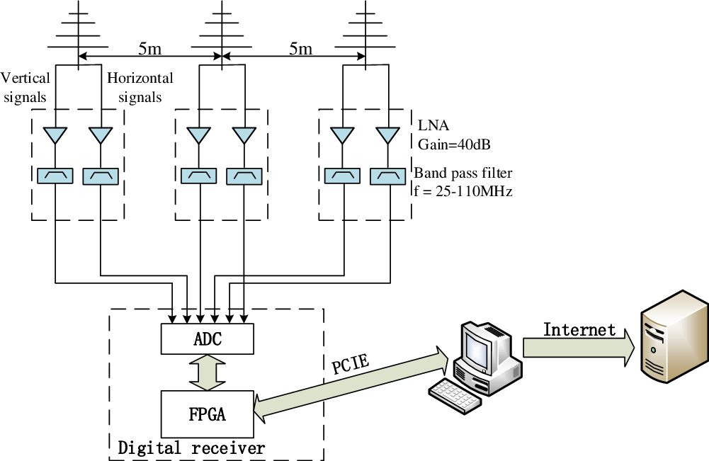
Figure 1. Overview of the solar radio burst observation system.

Figure 2. Prototype of the antenna array and LPDA parameters by simulation.

Figure 3. Simulated patterns of different antenna numbers at 30 MHz.
The system receiver unit contains the analog and digital signal processing electronic hardware to receive and process all RF signals from each antenna front end. The output from each LPDA is amplified to 40 dB with a low-noise amplifier, which has a flat gain in the range of 10–600 MHz with the gain flatness of $\pm$
0.8 dB. The noise figure of the amplifier is 1 dB. Then, the amplified signal is passed through a bandpass filter with a frequency range of 25–110 MHz to attenuate the spurious and unwanted RF signal outside the observation frequencies. The processed radio signals are transmitted by the analog receiving unit into the in-door digital receiver unit via underground cables to perform analog-to-digital conversion (ADC) and digital signal processing. The cables are placed in plastic pipes to slow the ageing process.
$\pm$
0.8 dB. The noise figure of the amplifier is 1 dB. Then, the amplified signal is passed through a bandpass filter with a frequency range of 25–110 MHz to attenuate the spurious and unwanted RF signal outside the observation frequencies. The processed radio signals are transmitted by the analog receiving unit into the in-door digital receiver unit via underground cables to perform analog-to-digital conversion (ADC) and digital signal processing. The cables are placed in plastic pipes to slow the ageing process.
Inside the digital receiver, all RF signals from the analog receiving unit are continuously sampled with a 250 MHz clock and quantised with 16 bits. The ADC acquisition card has sufficiently many channels to acquire the solar RF signal received by the arrays. The digital signal converted by ADC is entered into field programmable gate array (FPGA) for subsequent digital signal processing. The ADC is connected to the FPGA board through an FMC (FPGA Mezzanine Card) physical interface, which facilitates future system upgrades. The processed data are packaged and transmitted to the host computer via PCIe and stored in a 45-TB disk array. The daily observation period is 0–8 UT. Table 2 lists the characteristics of the system.
3. Digital receiver
3.1. Hardware
The digital receiver consists of an ADC acquisition card and an FPGA board, as shown in Figure 4. The acquisition card consists of four ADC ADS42LB69, each of which has two sampling channels and runs at a 250 MHz sampling clock per channel with a 16-bit quantised length. The FPGA is a Xilinx XCKU115 chip that has high arithmetic speed and abundant resources to support the processing of multiplexed data. The acquisition card and FPGA board are connected through the FMC physical interface, and their independence provides convenience for subsequent upgrades. The data exchange between the FPGA and the computer is completed by PCIE $\times$
8 lines.
$\times$
8 lines.
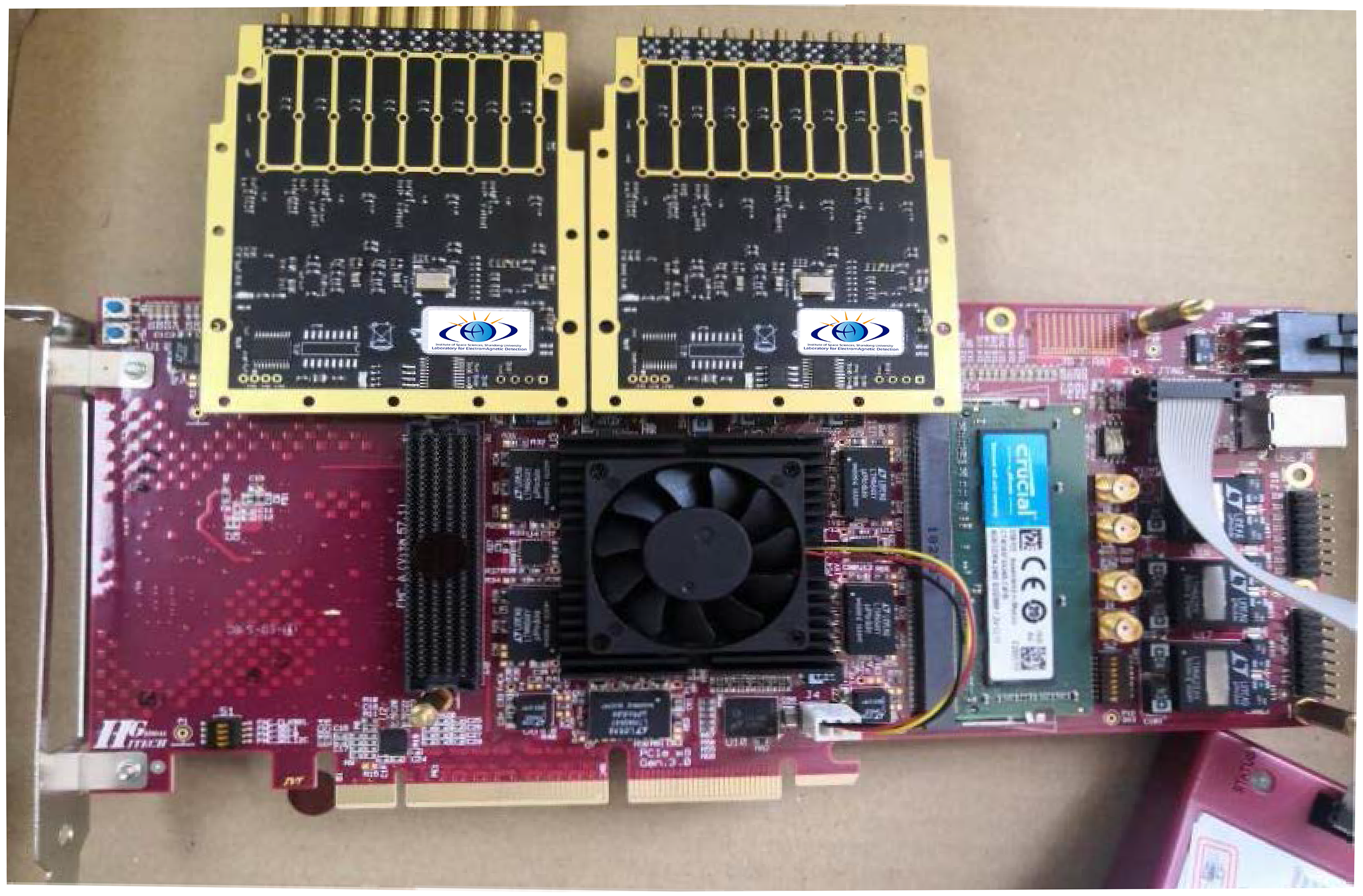
Figure 4. Digital Receiver Physical Diagram. The FPGA board is an HTG-830, and more information on the http://www.hitechglobal.com/Boards/Virtex-UltraScale-FPGA.htm.
3.2. Signal processing
The data processing flow of the digital receiver is shown in Figure 5. The digital signals converted by the ADC are finally transmitted to the FPGA. Then, the digital signals transmitted into the FPGA are processed by digital filtering, digital beamforming, digital polarisation synthesis and power spectrum accumulation to generate the dynamic spectrum. Finally, the processed data are packaged and transmitted to the computer via PCIe. The accumulation time is adjustable, which is controlled by the parameters issued by the computer to adjust the temporal resolution of the system to satisfy the requirements of different occasions.

Figure 5. Digital receiver physical diagram.
3.2.1. ADC sampling
In most cases of solar radio observations, low-frequency solar radio bursts have much stronger signal power than the quiet sun (by several tens of decibels). Therefore, the dynamic range of the ADC is an important parameter for the solar burst. The amplitude of the signal into the ADC should be set to an optimal level to retain a sufficient dynamic range of solar bursts and efficiently use the dynamic range of ADC. We tested the performance of the ADC in a frequency range of 15–450 MHz, and the parameters were obtained and are shown in Figure 6. The dynamic range of ADC is approximately 80 dB, which satisfies low-frequency solar bursts without power saturation.
Table 2. Characteristics of the system.


Figure 6. Performances of the receiving system at a $-1$
dBFS drive in the frequency range of 15–450 MHz.
$-1$
dBFS drive in the frequency range of 15–450 MHz.
3.2.2. Digital filter
In fact, the system has a bandpass filter with a frequency range of 25–110 MHz in the analog unit. The out-band suppression of filters greater than 40 dB can suppress most interference. However, there is still a strong interference near 15 MHz (Figure 8(a)). Here, we add digital filters to the digital receiver to suppress strong interference.
A prototype bandpass filter’s response is shown in Figure 7. The passband is 20–110 MHz. The attenuation of the stopband is more than 60 dB. The signals passed through a digital bandpass filter suppress strong interference. Figure 8(b) shows the effect of the filter. The strong interference at 15 MHz is suppressed by the digital filter.
3.2.3. Digital polarisation synthesis
The commonly used polarisation synthesis method is to use a 3-dB 90 $^{\circ}$
hybrid coupler. However, the hybrid coupler has the best effect at the centre frequency, and the phase difference at the sideband frequency is the largest, which results in inconsistent phase differences at different frequencies (Das et al. Reference Das, Roy, Keller and Tuccari2010; Zhang et al. Reference Zhang, Song, Du and Chen2018). This would greatly affect the subsequent data processing, especially the pointing accuracy of digital beamforming and the quality of solar radio observation data. Here, we use the digital polarisation synthesis method. Compared with analog polarisation synthesis, digital polarisation synthesis has the advantages of the same phase shift of each frequency point in the entire bandwidth, high precision and flexible adjustment. In addition, analog devices are not required, which reduces the impact of device noise and improves the quality of observation data.
$^{\circ}$
hybrid coupler. However, the hybrid coupler has the best effect at the centre frequency, and the phase difference at the sideband frequency is the largest, which results in inconsistent phase differences at different frequencies (Das et al. Reference Das, Roy, Keller and Tuccari2010; Zhang et al. Reference Zhang, Song, Du and Chen2018). This would greatly affect the subsequent data processing, especially the pointing accuracy of digital beamforming and the quality of solar radio observation data. Here, we use the digital polarisation synthesis method. Compared with analog polarisation synthesis, digital polarisation synthesis has the advantages of the same phase shift of each frequency point in the entire bandwidth, high precision and flexible adjustment. In addition, analog devices are not required, which reduces the impact of device noise and improves the quality of observation data.

Figure 7. The response of the bandpass filter.

Figure 8. Effect of the digital filter for the RFI.
We realise the digital polarisation synthesis in FPGA. First, the data acquired by ADC are converted into frequency domain data through FFT in FPGA. Then, each frequency point of one polarisation data is multiplied by a fixed 90° phase shift factor and added with another polarisation data to obtain the left/right circular polarisation signal, as shown in Figure 9. The RF cables in the system are made equal in length, and the analog devices use identical specifications. We consider that there are no amplitude and phase errors between channels. The number of FFT points determines the frequency resolution of the system and the accuracy of the digital polarisation synthesis. More FFT points can increase the accuracy. However, it will increase the resource consumption of the FPGA and temporal resolution of the system. Here, the number of FFT points for this system is 8 192.

Figure 9. Diagram of the polarisation synthesis realisation.
3.2.4. Digital beam forming
There will be a phase difference $\unicode{x03B2}=\tfrac{2\pi}{\lambda}d\sin\unicode{x03B8}$
between the solar signals received by the array antennas due to the geometric position. Here, d is the distance between adjacent antennas, and
$\unicode{x03B2}=\tfrac{2\pi}{\lambda}d\sin\unicode{x03B8}$
between the solar signals received by the array antennas due to the geometric position. Here, d is the distance between adjacent antennas, and $\unicode{x03B8}$
is the angle between the azimuth of the sun and the normal of the antenna array. Here, we use a digital beamforming algorithm to compensate for the phase difference. In earlier years, using analog phase shifters to complete beamforming was the main method, which was simple and easy to implement. In recent years, with the development of digital devices, digital beamforming technology has gradually replaced analog beamforming technology as a new mainstream due to its flexibility and high accuracy. Because
$\unicode{x03B8}$
is the angle between the azimuth of the sun and the normal of the antenna array. Here, we use a digital beamforming algorithm to compensate for the phase difference. In earlier years, using analog phase shifters to complete beamforming was the main method, which was simple and easy to implement. In recent years, with the development of digital devices, digital beamforming technology has gradually replaced analog beamforming technology as a new mainstream due to its flexibility and high accuracy. Because $\unicode{x03B8}$
is always changing as the position of the sun continues to change, the phase difference of the solar radio signal received by the adjacent antennas also changes in real time, which requires constant updating of the compensation factor (i.e. the weight vector of the digital beamforming) to compensate for the phase difference. We calculate the position coordinates of the sun at different times and further calculate the compensation factor of the phase difference. We divided the entire observation band into 25–35 MHz and 35–110 MHz. The weight vector of 25–35 MHz can be calculated by
$\unicode{x03B8}$
is always changing as the position of the sun continues to change, the phase difference of the solar radio signal received by the adjacent antennas also changes in real time, which requires constant updating of the compensation factor (i.e. the weight vector of the digital beamforming) to compensate for the phase difference. We calculate the position coordinates of the sun at different times and further calculate the compensation factor of the phase difference. We divided the entire observation band into 25–35 MHz and 35–110 MHz. The weight vector of 25–35 MHz can be calculated by
 \begin{equation}\unicode{x03C9}_n(k)=\frac{d_0}{d_i}\sum_{m=1}^M \unicode{x03C9}_0(m)\frac{\sin\!(\pi(k-1)d_0-(m-1)d_n)/d_n}{\pi\!(k-1)d_0-(m-1)d_n)/d_n},\end{equation}
where $k=1,2...,M$
, M is the number of antennas, and
$k=1,2...,M$
, M is the number of antennas, and $\unicode{x03C9}_0$
is the weight vector of the reference frequency, which are
$\unicode{x03C9}_0$
is the weight vector of the reference frequency, which are $\big[1,e^{j\frac{2\pi}{\lambda}d\ {\sin}\unicode{x03B8}},e^{j\frac{2\pi}{\lambda}2d\ {\sin}\unicode{x03B8}}\big]^T$
.
$\big[1,e^{j\frac{2\pi}{\lambda}d\ {\sin}\unicode{x03B8}},e^{j\frac{2\pi}{\lambda}2d\ {\sin}\unicode{x03B8}}\big]^T$
. $\unicode{x03B8}$
is the angle between the azimuth of the sun and the normal of the antenna array, which is changing with time. To reduce the side lobes, chebyshev weights are also used. Here, the reference frequency is 30 MHz.
$\unicode{x03B8}$
is the angle between the azimuth of the sun and the normal of the antenna array, which is changing with time. To reduce the side lobes, chebyshev weights are also used. Here, the reference frequency is 30 MHz.
Figure 10 shows the simulated digital beamforming pattern of 25–35 MHz. The synthesised beam main lobe is approximately 40 $^{\circ}$
. The synthetic beam enables 120
$^{\circ}$
. The synthetic beam enables 120 $^{\circ}$
azimuthal scanning.
$^{\circ}$
azimuthal scanning.
For 35–110 MHz, we use conventional beamforming, and the weight vector is 1. The bandwidth is too wide, which results in serious distortion of the pattern, and lower effectiveness than 25–35 MHz. We store these compensation factors in the FPGA and select the group of factors to call according to the time passed down by the computer.

Figure 10. Simulation pattern of 3-element beamforming.
3.3. Data format and interaction
The output of the digital receiver consists of both circular polarisation data. We use the self-defined file format and pack the data with timestamp and observation parameters such as polarisation tags and average times. The data are transmitted through PCIe to the computer. Each frame contains a complete set of spectrum data of 128 KB. Each raw-data file includes 4 096 frames of 512 MB. Next, we will convert the data format to flexible image transport system (FITS) format files, which is a unified standard format for data transmission and exchange between the world observatories as determined by the International Astronomical Union.
The data interaction between the digital receiver and the computer is realised by PCIe. The digital receiver transmits the spectrum data to the computer through PCIe, and the computer displays the spectrum map and stores the data. The upload rate of the dynamic spectrum data is approximately 31.5 MB s-1. The host computer is also responsible for the issuance of some control parameters, such as the acquisition time of the system and average number of spectrum. We also developed a remote operating programme for remote debugging.
4. Observations
The system runs normally for several months, and the daily observation period is $\sim$
0–8 UT. Several radio bursts have been observed by the system. Generally, solar radio bursts can be categorised into 5 fundamental types: type I, II, III, IV and V (Benz Reference Benz1986; Hamidi et al. Reference Hamidi, Ibrahim, Abidin, Ibrahim and Shariff2013). Here, we show type II bursts and type III bursts, which are most frequently observed at low frequencies. Type II bursts are observed in dynamic spectra as slowly drifting emission bands (Wild Reference Wild1950; Nelson & Melrose Reference Nelson and Melrose1985; Magdalenić et al. Reference Magdalenić2008; Mann et al. Reference Mann, Melnik, Rucker, Konovalenko and Brazhenko2018; Magdalenić et al. Reference Magdalenić2020). In addition to slowly drifting, type II bursts could be observed with distinctive features that are fundamental frequency (F) and harmonic frequency (H). The F and H bands are similar in frequency drifts, intensity behaviour and structure. Typically, type II bursts are associated with flare and CMEs (Wild, Smerd, & Weiss Reference Wild, Smerd and Weiss1963; Claß en & Aurass 2002; Chen et al. Reference Chen2014). Type III bursts are the most widely studied of all types of solar radio bursts and the most intense and frequently observed bursts. The signature feature is fast drifting from high frequency to low frequency. Type III bursts can occur as isolated events, groups of events or storms (Reid & Ratcliffe Reference Reid and Ratcliffe2014; Ansor et al. Reference Ansor, Hamidi and Shariff2021). The burst duration of an isolated burst is 1–3 s, while groups can last several minutes, and storms can last from 10 min to a few hours.
$\sim$
0–8 UT. Several radio bursts have been observed by the system. Generally, solar radio bursts can be categorised into 5 fundamental types: type I, II, III, IV and V (Benz Reference Benz1986; Hamidi et al. Reference Hamidi, Ibrahim, Abidin, Ibrahim and Shariff2013). Here, we show type II bursts and type III bursts, which are most frequently observed at low frequencies. Type II bursts are observed in dynamic spectra as slowly drifting emission bands (Wild Reference Wild1950; Nelson & Melrose Reference Nelson and Melrose1985; Magdalenić et al. Reference Magdalenić2008; Mann et al. Reference Mann, Melnik, Rucker, Konovalenko and Brazhenko2018; Magdalenić et al. Reference Magdalenić2020). In addition to slowly drifting, type II bursts could be observed with distinctive features that are fundamental frequency (F) and harmonic frequency (H). The F and H bands are similar in frequency drifts, intensity behaviour and structure. Typically, type II bursts are associated with flare and CMEs (Wild, Smerd, & Weiss Reference Wild, Smerd and Weiss1963; Claß en & Aurass 2002; Chen et al. Reference Chen2014). Type III bursts are the most widely studied of all types of solar radio bursts and the most intense and frequently observed bursts. The signature feature is fast drifting from high frequency to low frequency. Type III bursts can occur as isolated events, groups of events or storms (Reid & Ratcliffe Reference Reid and Ratcliffe2014; Ansor et al. Reference Ansor, Hamidi and Shariff2021). The burst duration of an isolated burst is 1–3 s, while groups can last several minutes, and storms can last from 10 min to a few hours.
Figure 11 shows the background-subtracted dynamic spectrum of type III bursts observed by this system. Figure 11(a) shows a group of type III bursts observed on 29 August 2021 during the interval $\sim$
02:21–02:24 UT. The frequencies of type III are
$\sim$
02:21–02:24 UT. The frequencies of type III are $\sim$
30–110 MHz. Figure 11(b) shows an isolated type III burst recorded at 03:21 UT on 20 December 2021. This type III burst lasts for a short duration, and the frequency range was
$\sim$
30–110 MHz. Figure 11(b) shows an isolated type III burst recorded at 03:21 UT on 20 December 2021. This type III burst lasts for a short duration, and the frequency range was $\sim$
30–100 MHz.
$\sim$
30–100 MHz.
Observation systems with high temporal and frequency resolutions are particularly important for studying the fine structures of solar radio bursts. In Figure 12(a), we show the fine structure of the type III burst in Figure 11(b) for the chosen frequency of 30–110 MHz. The burst started at 03:20:44 (UT), and Learmonth simultaneously observed this burst (shown in Figure 12(b)). In Figure 12(c), we show the millisecond burst structures at 03:20:56. The time scale in the graph is 1 000 ms with 250 spectra. We can see the difference in radiation intensity at different frequencies and the variation with time. The fine structure of the burst is clearly visible.

Figure 11. Dynamic spectra of type III bursts observed by the system at the CSO with a temporal resolution of 4 ms and a frequency resolution of 30 kHz. The horizontal axis represents time, the vertical axis represents frequency, and the colours represent different solar radio intensities at different frequencies.

Figure 12. Fine structure of type III burst in Figure 11(b) observed on 20 December 2021.
Figure 13 is a type II burst observed by the system on 9 October 2021 during the interval $\sim$
06:34–06:46 UT. The burst was observed at frequencies from 115 to 25 MHz. This type II burst (Figure 13) is triggered during an M1.6-class flare observed by the Geostationary Operational Environmental Satellites (GOES). The M1.6 class flare started at 06:19 UT and stopped at 06:53 UT, with a peak at 06:38 UT. The X-ray flux at the burst time is also shown in Figure 13. The result is indicated by red line. We can see that type II burst occurs near the peak of the flare.
$\sim$
06:34–06:46 UT. The burst was observed at frequencies from 115 to 25 MHz. This type II burst (Figure 13) is triggered during an M1.6-class flare observed by the Geostationary Operational Environmental Satellites (GOES). The M1.6 class flare started at 06:19 UT and stopped at 06:53 UT, with a peak at 06:38 UT. The X-ray flux at the burst time is also shown in Figure 13. The result is indicated by red line. We can see that type II burst occurs near the peak of the flare.

Figure 13. Type II burst observed by the system on 9 October 2021 and the X-ray flux. The red line in the figure is the X-ray flux.
The observing system has high resolutions, and burst data were obtained. These data can be corroborated with data from other stations such as Learmonth, which has similar observation periods to verify the correctness of the burst data. These data also support scientific research. In addition, the observatory is located at 112 E with a daily observation time of 0–8 (UT), and it can supplement the solar observation data during this period. Moreover, the system is a low-frequency solar observation system worked at 25–110 MHz. In cooperation with other high-frequency solar radio spectrum observation systems, a complete burst structure can be obtained.
5. Summary and discussion
Spectral observations with high temporal and frequency resolutions are of great significance for studying the fine structures of solar radio bursts. It is helpful to understand many physical processes in the burst region and solve scientific problems remain unresolved. Many solar radio spectrographs have been established around the world to observe the dynamic spectra of solar radio bursts. However, many of them were established 1-2 decades ago and limited by the electronic and digital technologies at that time, so the temporal resolution and frequency resolution were low. Thus, the fine structures of the bursts are difficult to observe.
We propose a new low-frequency solar radio burst observation system in this paper, which is located in Chashan Solar Observatory (CSO), Weihai City, China. The system uses digital technology to realise the function of analog devices. Hence, we can reduce the interference caused by analog devices and improve the flexibility of the system. Furthermore, the system has high temporal resolution (up to 0.2 ms) and frequency resolution ( $\sim$
30 kHz). Of course, the cost of the system is high. Several bursts have been observed by the system, and some of them are shown in this paper. The obtained spectra can be used to study the fine structure of solar radio bursts and forecast the space weather. The daily observation period is 0–8 UT. Meanwhile, the time synchronisation function is added to the system, which lays the foundation for low-frequency coherence with other stations.
$\sim$
30 kHz). Of course, the cost of the system is high. Several bursts have been observed by the system, and some of them are shown in this paper. The obtained spectra can be used to study the fine structure of solar radio bursts and forecast the space weather. The daily observation period is 0–8 UT. Meanwhile, the time synchronisation function is added to the system, which lays the foundation for low-frequency coherence with other stations.
Through daily observation for approximately half a year, some problems were found. The RFI becomes worse, which leads to weak bursts difficult to be detected. The main sources of RFI are FM radio and fishermen communications, which are mainly single-frequency signals. Methods to reduce RFI should be considered in this observation system soon. We are considering the adaptive LMS filtering algorithm, which has good suppression effect on single-frequency interference. Its advantages are the simple structure and easy implementation. Next, we will use the offline data of CSO to test the algorithm. If it works well, we will apply it to our system. In addition, the impact of the amplitude and phase errors caused by cables and analog devices between channels on the system accuracy should be evaluated in the next step. We will study the theory of the correction if necessary. When the system runs maturely, the number of antennas will increase to eight to improve the sensitivity.
Acknowledgement
This work is supported by the National Natural Science Foundation of China 41904158, 42127804, 11803017; Shandong postdoctoral innovation project 202002004 and Young Scholars Program of Shandong University, Weihai 20820201005. We also thank Prof. Qingfu Du, Dr. Shiwei Feng and Dr. Junrui Zhang for the antenna installation as well as the infrastructural construction of the observation system. Thanks to Jie Liu for the spectrometer.


