


1. Introduction
1.1. Context
My aim with this review is to unify the various observational and simulation approaches for investigating the stellar initial mass function (IMF), the mass distribution of stars arising from a star formation event. I do this by summarising work over the past few decades focusing primarily on observational constraints, and presenting a self-consistent framework to support future research. I address issues of terminology, definition, and scope of results in a way not previously attempted, with the goal of minimising ambiguity and assessing the degree of consistency or otherwise in published results regarding the ‘universality’ of the IMF.
The significance of understanding the IMF was highlighted by Kennicutt (Reference Kennicutt, Gilmore and Howell1998) who wrote: ‘Accurate knowledge of the form and mass limits of the stellar initial mass function, and its variation in different star formation environments, is critical to virtually every aspect of star formation, stellar populations, and galaxy evolution’. And: ‘Testing the universality of this initial mass function remains as our primary challenge for the coming decade’. Despite this goal being set two decades ago, the question of the universality of the IMF is still unresolved with a variety of results over the past decade providing evidence in favour of some kind of variation (e.g. van Dokkum & Conroy Reference van Dokkum and Conroy2010; Treu et al. Reference Treu, Auger, Koopmans, Gavazzi, Marshall and Bolton2010; Gunawardhana et al. Reference Gunawardhana2011). Kennicutt (Reference Kennicutt, Gilmore and Howell1998) concluded that, while there was no clear physical reason to expect the IMF to be universal, there was also ‘no compelling evidence for large systematic IMF variations in galaxies’. A contrary view was expressed by Larson (Reference Larson1998) who summarised a broad range of circumstantial evidence in favour of a stellar IMF with proportionally more high-mass stars at high-redshift compared to the low-redshift IMF.
The challenge posed in understanding the IMF is highlighted through the range and frequency of review articles dedicated to it since the 1980s (Scalo Reference Scalo, De Loore, Willis and Laskarides1986, Reference Scalo, Gilmore and Howell1998; Kennicutt Reference Kennicutt, Gilmore and Howell1998; Larson Reference Larson1998; Kroupa Reference Kroupa2002; Chabrier Reference Chabrier2003a) with a growing number in recent years (McKee & Ostriker Reference McKee and Ostriker2007; Elmegreen Reference Elmegreen2009; Bastian, Covey, & Meyer Reference Bastian, Covey and Meyer2010; Jeffries Reference Jeffries, Reylé, Charbonnel and Schultheis2012; Kroupa et al. Reference Kroupa, Weidner, Pflamm-Altenburg, Thies, Dabringhausen, Marks and Maschberger2013; Offner et al. Reference Offner, Clark, Hennebelle, Bastian, Bate, Hopkins, Moraux and Whitworth2014; Krumholz Reference Krumholz2014), each touching on different but crucial aspects of the problem. Major conferences, too, have focussed on the IMF, with a celebration of the 50th anniversary of the IMF concept in 2005, ‘The Initial Mass Function 50 Years Later’ (Corbelli, Palla, & Zinnecker Reference Corbelli, Palla and Zinnecker2005), updating work presented in 1998 at the ‘The Stellar Initial Mass Function (38th Herstmonceux Conference)’ (Gilmore & Howell Reference Gilmore and Howell1998). This was followed in 2010 with ‘UP2010: Have Observations Revealed a Variable Upper End of the Initial Mass Function?’ exploring evidence for the possibility of IMF variations (Treyer et al. Reference Treyer, Wyder, Neill, Seibert and Lee2011), and in 2016 with a Lorentz Centre workshop ‘The Universal Problem of the Non-Universal IMF’Footnote a to share updates on the status of the work on IMF variations. Such levels of activity provide further evidence for the significance of the IMF and the complexity involved in understanding its details.
The field of IMF studies is vast. A search using the SAO/NASA Astrophysics Data System for papers having abstracts containing ‘initial mass function’ or ‘IMF’ yields more than 15 000 publications. No single reviewer could ever hope to comprehensively summarise such a prodigious volume of work. Fortunately, existing reviews cover a broad range of different aspects of the field, and provide a solid basis on which to build.
By way of illustration, Elmegreen (Reference Karlsson, Bromm and Bland-Hawthorn2009) summarises and compares the shape of the IMF (its slope and characteristic mass) as probed through an extensive range of measurements within and external to the Milky Way and gives a high-level review of the primary physical processes responsible for star formation and the IMF. Bastian et al. (Reference Bastian, Covey and Meyer2010) provides a comprehensive review into the question of the universality of the IMF, thoroughly summarising work in the Galaxy and Local Group along with much of the work that was developing at the time to explore novel extragalactic approaches. Subsequently, these fields have evolved quickly, with a lot of attention on the IMF shape in early-type galaxies in particular. Kroupa et al. (Reference Kroupa, Weidner, Pflamm-Altenburg, Thies, Dabringhausen, Marks and Maschberger2013) present an extensive and detailed review ranging from defining the IMF through to the various approaches to measuring the IMF in both stellar and extragalactic regimes, and discuss the implications in the context of the ‘integrated galaxy IMF’ (IGIMF) formalism of Kroupa & Weidner (Reference Kroupa and Weidner2003). Offner et al. (Reference Offner, Clark, Hennebelle, Bastian, Bate, Hopkins, Moraux and Whitworth2014) present a detailed summary of work measuring the IMF in Milky Way star clusters and nearby galaxies, along with an overview of extragalactic work, before providing a highly comprehensive analysis of analytical and numerical theories behind the form and origins of the IMF. Krumholz (Reference Krumholz2014) reviews in detail the physical processes and phenomenology of star formation, and the status of the theoretical framework used in addressing the problem.
This review is intended to complement these and other reviews, referring to the detailed summaries they provide as needed, without attempting to duplicate the scope of their work. The aim here is not to deliver a comprehensive review of a vast body of work, but rather to synthesise the key elements from the work to date in order to develop a self-consistent framework and set of terminology on which to base future work. It is inevitable that there will be incompleteness in the references covered below, but the hope is that the main elements are addressed, and that at least representative results are presented.
1.2. Scope of this review
This review builds on earlier work by summarising traditional approaches and the growing range of more recent techniques used to measure or infer the IMF with the aim of establishing their strengths and limitations, and identifying the different regimes in which they are applicable. I explore issues around the nature of the problem itself, in particular the degree to which the IMF is even a well-posed concept and whether there is an alternative formalism that might lend itself better to observational measurement.
The strengths and limitations of different methods are highlighted, and comparisons made between the typical samples to which they are applied, and the corresponding range of physical conditions probed. Some examples include the approaches typically used in stellar investigations within the Milky Way and Local Group galaxies, contrasted against those now becoming routine in extragalactic analyses. The latter include metrics relying on stellar population synthesis (SPS) tools (e.g. Hoversten & Glazebrook Reference Hoversten and Glazebrook2008; van Dokkum & Conroy Reference van Dokkum and Conroy2010; Gunawardhana et al. Reference Gunawardhana2011), the comparison of stellar and dynamical mass-to-light ratios (e.g. Treu et al. Reference Treu, Auger, Koopmans, Gavazzi, Marshall and Bolton2010), kinematics of stellar populations to infer mass-to-light ratios (e.g. Cappellari et al. Reference Cappellari2012), and galaxy census approaches such as the cosmic star formation history (SFH) and the cosmic stellar mass density (SMD) evolution (e.g. Wilkins, Trentham, & Hopkins Reference Wilkins, Trentham and Hopkins2008a; Wilkins et al. Reference Wilkins, Hopkins, Trentham and Tojeiro2008b).
I investigate the potential for linking the results established from this broad range of approaches, highlighting areas of actual inconsistency and carefully defining areas where apparent inconsistencies are potentially a result of different physical conditions accessible to different methodologies. I then identify opportunities for development of the field through new approaches to measurement of the IMF to provide a self-consistent and uniform foundation for subsequent work.
The review is structured as follows. In Section 2, I briefly summarise the history of the IMF, explore issues of nomenclature, and propose some conventions to minimise ambiguities in future work. Sections 3–7 present an overview of the wide variety of measurement approaches taken to date to constrain the IMF. I present a updated approach to the IMF in Section 8, followed by a discussion in Section 9 of the constraints and implications from the numerous measurements to date, before concluding in Section 10. I assume H 0 = 70 km s−1 Mpc−1, ΩM = 0.3 and ΩΛ = 0.7 where necessary for converting between redshift and lookback time.
2. Background and challenges
2.1. Overview and history
Stars and star clusters form when dense gas collapses through gravitational or turbulent processes. The physical state of the gas (including temperature, pressure, metallicity, and turbulence) determines which pockets of gas fragment and collapse, and so ultimately the masses of the stars formed. Since the evolution of a single star is almost entirely determined by its initial mass (although binary effects also play a role), and the distribution of mass within a bound system defines its kinematics, the evolution of a cluster of coeval stars is determined almost entirely by its stellar IMF. The evolution of a galaxy composed of such clusters depends intimately on this (potentially varying) IMF in combination with its SFH.
The IMF establishes the fraction of mass sequestered in sub-solar-mass stars (down to masses as little as 0.1 M⊙) with lifetimes much greater than the age of the Universe, and the high-mass fraction (stars up to 120 M⊙ or perhaps more) that rapidly become supernovae, returning chemically enriched gas to the interstellar medium to support subsequent generations of star formation. The less numerous higher mass stars dominate the light from a star cluster or a galaxy, but the more numerous lower mass stars dominate the mass. This results in a need for different tracers to probe the high- and low-mass regimes of the IMF. It also means that the mass-to-light ratio is sensitive to the IMF shape.
The IMF is consequently the fundamental concept linking each of: (1) the process of star formation itself through the conversion of molecular clouds (enriched to some degree by heavy elements) into a population of stars; (2) feedback and chemical enrichment processes arising from the radiative and mechanical energy returned to the interstellar medium through stellar winds and supernovae from existing stellar populations that influence subsequent generations of stars and their metallicity; (3) the measurements used to convert observables (such as broadband luminosities or spectral line measurements), to underlying physical quantities (such as the current rate of star formation and total stellar mass), in order to enable studies of star formation and galaxy evolution.
The IMF was first measured by Salpeter (Reference Salpeter1955) while working at the Australian National University, by measuring the luminosity distribution of stars in the solar neighbourhood. It was shown to be consistent with a power law over the mass range 0.4 ≲ m/M⊙ ≲ 10. Numerous measurements of the IMF over the subsequent sixty years (e.g. Miller & Scalo Reference Miller and Scalo1979; Scalo Reference Scalo, De Loore, Willis and Laskarides1986; Basu & Rana Reference Basu and Rana1992; Kroupa, Tout, & Gilmore Reference Kroupa, Tout and Gilmore1993) show that this power law does not extend to the lowest masses but has a flatter slope below about half a solar mass. The original power law slope for high-mass stars found by Salpeter extends up to about 120 solar masses (e.g. Scalo Reference Scalo, De Loore, Willis and Laskarides1986, Reference Scalo, Gilmore and Howell1998; Kroupa Reference Kroupa2001; Chabrier Reference Chabrier2003a), although with some variation (but also large observational uncertainties) in the reported high-mass slope and upper mass limit, and some debate about the value for the characteristic or ‘turn over’ mass.
While much of the observational work on the IMF in the late 20th century focused on this same method of using resolved star counts as the most robust and direct approach available, Kennicutt (Reference Kennicutt1983) pioneered an approach using integrated galaxy light. Many alternatives were also explored, as summarised by Scalo (Reference Scalo, De Loore, Willis and Laskarides1986) and Kennicutt (Reference Kennicutt, Gilmore and Howell1998). These include a range of approaches such as ultraviolet (UV) luminosities of galaxies (Donas & Deharveng Reference Donas and Deharveng1984), indirect approaches related to chemical evolution and abundance ratios (Audouze & Tinsley Reference Audouze and Tinsley1976), and others like galaxy mass-to-light ratios that are now more routinely used to estimate IMF properties (e.g. Treu et al. Reference Treu, Auger, Koopmans, Gavazzi, Marshall and Bolton2010).
The IMF was also used as a probe of cosmology and dark matter. For example, constraints on the IMF and cosmology were inferred from the evolution of galaxy colours (Tinsley Reference Tinsley1972), number counts of galaxies (Guiderdoni & Rocca-Volmerange Reference Guiderdoni and Rocca-Volmerange1990), and the form of the IMF was invoked to explore the extent to which stellar remnants (e.g. Dantona & Mazzitelli Reference Dantona and Mazzitelli1986) or substellar objects (e.g. Staller & de Jong Reference Staller and de Jong1981) could explain the ‘missing matter’ in the solar vicinity (Bahcall Reference Bahcall1984). The cosmological constraints associated with the IMF are no longer compelling in the age of precision cosmology (e.g. Schmidt et al. Reference Schmidt1998; Planck Collaboration et al. 2016). Likewise, as the numbers of substellar objects have been progressively constrained by observations (e.g. Tinney Reference Tinney1993; Kroupa et al. Reference Kroupa, Tout and Gilmore1993) and other approaches matured in ruling out stellar-related contributions to possible baryonic dark matter (Graff & Freese Reference Graff and Freese1996a, Reference Graff and Freese1996b; Alcock et al. Reference Alcock2000, Reference Alcock2001), this aspect of the IMF has also become less important. With the establishment of the now standard ΛCDM model, the focus on the IMF now is primarily connected to the physics of star formation and galaxy evolution.
Part of the challenge in understanding the IMF as currently conceived is that it is a fundamentally statistical concept and not directly observable. Elmegreen (Reference Karlsson, Bromm and Bland-Hawthorn2009) notes that when estimating the IMF for star clusters, ‘no cluster IMF has ever been observed throughout the whole stellar mass range’. He explains that to probe the upper mass range of the IMF needs a very massive cluster, which are rare systems, with the nearest being too far away (a few kpc) to see the low-mass stars. Conversely the nearest clusters, required for measuring the low-mass end of the IMF, are all low-mass clusters having few high-mass stars. He concludes: ‘Until we can observe the lowest mass stars in the highest mass clusters an IMF makes sense only for an ensemble of clusters or stars’. It is notable that the science cases for the next generation of major telescope facilities, James Webb Space Telescope (JWST), Giant Magellan Telescope (GMT), Thirty Metre Telescope (TMT), European Large Telescope (ELT), all include the goal of studying resolved star formation in such high-mass Galactic star clusters. Kroupa et al. (Reference Kroupa, Weidner, Pflamm-Altenburg, Thies, Dabringhausen, Marks and Maschberger2013) take this concept a step further and detail why the IMF is not ever a measurable quantity, by noting that star formation occurs on Myr timescales. This means that for stellar systems younger than about 1Myr, star formation has not ceased and so the IMF is not yet assembled, while for systems older than about 0.5 Myr, higher mass stars are lost through stellar evolutionary effects, while dynamical processes can also cause the loss of lower mass stars. This means that there is no single time at which the full ensemble of masses is present and measurable within a discrete spatial volume. There is hence a need to address the issue of the short but finite time of formation, together with the fact that star clusters do not form in isolation (typically) but within a complex, multiphase interstellar medium that is also influenced by, and influencing, adjacent sites of star formation.
A possible solution to this issue arises through considering how many independent samples are required, and over what spatial scale they must be probed, in order to infer the IMF robustly. By sampling a sufficiently large number of star-forming regions it might be expected that each evolutionary stage is captured and the ensemble can be used to infer the underlying IMF. Kruijssen & Longmore (Reference Kruijssen and Longmore2014) describe a general formalism, which they apply to star formation scaling relations in galaxies, that links the timescale of different phases of a process with the number of independent samples required to capture all temporal phases and the spatial scale on which the processes are measured. They note that ‘[star formation] relations measured in the solar neighbourhood are fundamentally different from their galactic counterparts’ and conclude that ‘… when a macroscopic correlation is caused by a time evolution, then it must break down on small scales because the subsequent phases are resolved’. Considering the temporal dependencies of star formation and the range of spatial scales over which we are interested in characterising it, it may be that the formalism and concept of the IMF itself may need to be restructured (Scalo Reference Scalo, Gilmore and Howell1998).
Despite these difficulties, a range of the early approaches towards inferring the IMF have been refined over the past decade and are now used routinely. These include an update of the Kennicutt (Reference Kennicutt1983) approach used by Hoversten & Glazebrook (Reference Hoversten and Glazebrook2008) and Gunawardhana et al. (Reference Gunawardhana2011), use of the Wing–Ford band to infer dwarf-to-giant ratio (e.g. Cenarro et al. Reference Cenarro, Gorgas, Vazdekis, Cardiel and Peletier2003; van Dokkum & Conroy Reference van Dokkum and Conroy2010; Smith, Lucey, & Carter Reference Smith, Lucey and Carter2012) following the early work of Whitford (Reference Whitford1977), use of kinematics (e.g. Cappellari et al. Reference Cappellari2012), gravitational lensing observations (e.g. Treu et al. Reference Treu, Auger, Koopmans, Gavazzi, Marshall and Bolton2010; Smith & Lucey Reference Smith and Lucey2013), chemical abundance constraints (e.g. Portinari, Sommer-Larsen, & Tantalo Reference Portinari, Sommer-Larsen and Tantalo2004a; Komiya et al. Reference Komiya, Suda, Minaguchi, Shigeyama, Aoki and Fujimoto2007; Sliwa et al. Reference Sliwa, Wilson, Aalto and Privon2017), and more. The 2.3 μm CO index has also been proposed for probing the dwarf-to-giant ratio (Kroupa & Gilmore Reference Kroupa and Gilmore1994; Mieske & Kroupa Reference Mieske and Kroupa2008). In the same period other novel approaches have been developed, such as those using cosmic census measurements to place constraints on the IMF (e.g. Baldry & Glazebrook Reference Baldry and Glazebrook2003; Hopkins & Beacom Reference Hopkins and Beacom2006; Wilkins et al. Reference Wilkins, Trentham and Hopkins2008a, Reference Wilkins, Hopkins, Trentham and Tojeiro2008b).
With this explosion in the range of approaches now being used to measure or infer the IMF, there has been a related growth in the tension between apparently conflicting results. One example is a need for so-called ‘top-heavy’ IMFs (a relative excess of high-mass stars compared to the nominal Salpeter IMF) in regions of elevated star formation rate (SFR) (e.g. Gunawardhana et al. Reference Gunawardhana2011) that contrasts with the so-called ‘bottom-heavy’ IMFs (a relative excess of low-mass stars) inferred in the cores of massive elliptical galaxies (e.g. van Dokkum & Conroy Reference van Dokkum and Conroy2012). It is less clear whether such results are actually in conflict or not. The different approaches measure different things, and the spatial scales probed are different as is the epoch for the star formation activity. The current review is aimed at assessing the available wealth of different metrics and their results in a self-consistent fashion, to begin to unify our approach to understanding the IMF.
With this context in mind it is first necessary to review the terminology used in discussing the IMF and to explore conventions of nomenclature.
2.2. IMF definitions and terminology
At its most concrete, the IMF can be defined as the mass distribution of stars arising from a star formation event. It has been described and inferred in this sense from observational measurements by innumerable authors over more than sixty years (e.g. Salpeter Reference Salpeter1955; Miller & Scalo Reference Miller and Scalo1979; Kennicutt Reference Kennicutt1983; Scalo Reference Scalo, De Loore, Willis and Laskarides1986; Kroupa Reference Kroupa2001; Chabrier Reference Chabrier2003a), who have found that the IMF in many cases follows a similar form and established the broad properties of this distribution. In general, the IMF has a declining power law shape for masses above about 1 M⊙, with a flatter slope at lower masses down to some minimum mass. Below the stellar/sub-stellar boundary brown dwarfs are often now included in IMF estimates (e.g. Kroupa et al. Reference Kroupa, Weidner, Pflamm-Altenburg, Thies, Dabringhausen, Marks and Maschberger2013), with a more positive slope below the hydrogen burning mass limit (although the shape at the lowest masses may be more complex, e.g. Drass et al. Reference Drass, Haas, Chini, Bayo, Hackstein, Hoffmeister, Godoy and Vogt2016). The observed mass function across the stellar/sub-stellar boundary may be a superposition of two physically distinct IMFs, inferred from the deficit in models compared to observations of brown dwarfs that form through direct gravitational collapse in molecular clouds (Thies et al. Reference Thies, Pflamm-Altenburg, Kroupa and Marks2015). The general shape and key parameters of the IMF are illustrated in Figure 1.
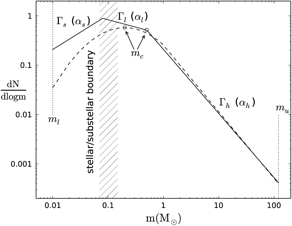
Figure 1. An illustration of the key aspects of the IMF as it has been parameterised, either as a piecewise series of power law segments (e.g. Kroupa Reference Kroupa2001) or a log-normal at low masses with a power law tail at high masses (e.g. Chabrier Reference Chabrier2003a).
Many authors have summarised the range of functional forms used to parameterise the IMF, with the common choices being piecewise power laws (e.g. Kroupa et al. Reference Kroupa, Weidner, Pflamm-Altenburg, Thies, Dabringhausen, Marks and Maschberger2013, their equations 4 and 5) or a log-normal form (e.g. Chabrier Reference Chabrier2003b, Reference Chabrier, Corbelli, Palla and Zinnecker2005). Alternative functional forms have been proposed with varying motivations (e.g. De Marchi, Paresce, & Portegies Zwart Reference De Marchi, Paresce, Portegies Zwart, Corbelli, Palla and Zinnecker2005; Parravano, McKee, & Hollenbach Reference Parravano, McKee and Hollenbach2011; Maschberger Reference Maschberger2013) that largely provide the same practical functionality as the more commonly used forms.
Key parameters are: (1) the lower mass limit, ml, typically chosen as ml = 0.08 M⊙ or ml = 0.01 M⊙ (unless substellar objects are included, in which case ml = 0.01 M⊙ is common); (2) the upper mass limit, mu, with typical values of mu = 100 M⊙, mu = 120 M⊙ or mu = 150 M⊙; (3) mc, the characteristic mass, which is the peak in the lognormal form, or the ‘turn over’ mass where the slope of the power law representation changes (although as seen in Figure 1 this isn’t necessarily an actual turn over in the relation), with mc ranging from about 0.2–1 M⊙ depending on the formalism chosen, and mc = 0.5 M⊙ common in the power law representation; (4) the slope parameters for each segment of a piecewise power law relation, or the equivalent in the lognormal relation defining the width of the relation at low masses, and the power law slope at high masses. Here and throughout I use αs for the substellar power law slope, αl for the low-mass slope, and αh for the high-mass slope (noting mc for clarity when relevant). This choice avoids a numerical sequence in which α 1 (say) is ambiguous depending on the value of ml, i.e., whether the IMF in question includes substellar masses or not. Where a single power law spanning more than one of these segments is assumed, I use α and define the mass range explicitly.
The same functional form for the mass distribution of stars formed in a single star-forming region and called ‘the IMF’ is also used to describe the average mass distribution of stars formed across a galaxy, a concept sometimes referred to as the ‘integrated galaxy IMF’ or IGIMF (Kroupa & Weidner Reference Kroupa and Weidner2003), as well as to the effective average stellar mass distribution for a population of galaxies, referred to as the ‘cosmic IMF’ (Wilkins et al. Reference Wilkins, Hopkins, Trentham and Tojeiro2008b). If the IMF is universal, these quantities may be identicalFootnote b but not otherwise. Such broad application of the term ‘IMF’, validated through an underlying presumption of an IMF that is ‘universal’ until proven otherwise, may actually be hampering attempts to further understand the properties of the IMF including whether or not it varies. I return to this point below in Sections 2.4 and 8.
Other issues that hamper progress arise from inconsistent conventions describing the IMF. This field suffers from a wide range of such inconsistencies, and these seem to be growing in number rather than converging as the breadth of investigations increases. In an effort to stem this flow, I explicitly address these next.
2.3. Conventions and language usage
Ambiguities in the way the IMF is discussed unnecessarily complicate what is already a complex problem. Different authors adopt different conventions or approaches to the description of the IMF. Different language is used to describe the same quantity, mass ranges are omitted or assumed implicitly, and ambiguous terms are introduced. While not a fundamental problem, this definitely leads to confusion and the potential for misinterpretation, which can be easily avoided if clear conventions and unambiguous language are used. That this point has been made repeatedly by different authors (e.g. Kennicutt Reference Kennicutt, Gilmore and Howell1998; Bastian et al. Reference Bastian, Covey and Meyer2010) and still bears repeating is evidence that it deserves attention. Similar issues of convention and usage have been recognised by the cosmology community (Croton Reference Croton2013), emphasising the importance of striving for clarity.
Here I recount a number of sources of potential confusion and make recommendations for avoiding ambiguity, while acknowledging that the majority of authors do tend to be diligent. The bottom line, though, is that because of the many potential sources of confusion in this field there is an especial need for authors, referees, and editors to make extra effort to ensure clarity and consistency.
2.3.1. Sign conventions
Different authors have adopted a variety of nomenclature to represent the shape and power law slope(s) of the IMF, and in particular whether or not a negative sign is given in the power law definition or appears in the parameter. Opposing sign conventions may even appear within a single publication (e.g. Elmegreen Reference Elmegreen2009; Turner Reference Turner2009). This can lead to unnecessary confusion, especially when discussing the exponent of a power law slope in a distribution that has opposite signs at the low-mass and high-mass ends. It is worth noting that opposing conventions for the use of the negative sign have existed almost as long as work in this field. Salpeter (Reference Salpeter1955) did not use a pronumeral descriptor for the power law slope at all, but provided the power law value explicitly in his Equation (5), a choice followed by Kennicutt (Reference Kennicutt1983). Audouze & Tinsley (Reference Audouze and Tinsley1976) and Tinsley (Reference Tinsley1977) give the negative sign in the equation, a choice subsequently recommended by Kennicutt (Reference Kennicutt, Gilmore and Howell1998), but Miller & Scalo (Reference Miller and Scalo1979), Scalo (Reference Scalo, De Loore, Willis and Laskarides1986), and Kennicutt, Tamblyn, & Congdon (Reference Kennicutt, Tamblyn and Congdon1994) use the convention that any sign is incorporated into the slope parameter.
I strongly recommend that, to minimise ambiguity, all authors adopt the latter convention (following, e.g. Scalo Reference Scalo, De Loore, Willis and Laskarides1986; Kennicutt et al. Reference Kennicutt, Tamblyn and Congdon1994):
 \begin{equation} {{{\rm{d}}N} \over {{\rm{d}}m}} \propto {\left( {{m \over {{{\rm{M}}_ \odot }}}} \right)^\alpha }{\rm{a}}nd \end{equation}
 \begin{equation} {{{\rm{d}}N} \over {{\rm{d}}\log m}} \propto {\left( {{m \over {{{\rm{M}}_ \odot }}}} \right)^\Gamma }, \end{equation}
where Γ = α + 1 and the original Salpeter slope is α = −2.35 or Γ = −1.35. Contrary to some recent usage (e.g. Bastian et al. Reference Bastian, Covey and Meyer2010; Kroupa et al. Reference Kroupa, Weidner, Pflamm-Altenburg, Thies, Dabringhausen, Marks and Maschberger2013), the negative sign is not included in the relations adopted here and appears in the quantities α and Γ explicitly. This convention has the advantage that the sign of the parameter and of the power law itself are the same, not opposing. It ensures that a sign change from the lowest masses to the highest masses (e.g. in a piecewise power law description) is in the sense that intuition would suggest. It avoids inconsistencies or clumsy presentation when discussing the value of the power law slope as contrasted with the value of the parameter, or when inequalities are used to describe slopes flatter or steeper than some nominal parameter value. It eliminates confusion over the need to swap the sense of asymmetric errors in estimates of the parameter as opposed to the actual slope. For internal self-consistency and ease of comparison between published results, I present all IMF slopes discussed throughout using α as defined above.
2.3.2. IMF naming conventions
The use of the phrases ‘Salpeter IMF,’ ‘universal IMF,’ ‘typical IMF,’ ‘normal IMF,’ or ‘standard IMF’, often interchangeably, can be confusing because of the varying assumptions made in relation to the stellar mass range and whether or not a slope change is assumed at the low-mass end. Sometimes what is meant is the Salpeter power law slope over a given mass range (typically 0.1 < m/M⊙ < 100), but also sometimes extending up to 120 – 150 M⊙, and often including other implicit assumptions. Common omissions that lead to ambiguity include the mass range being assumed, the existence or degree of a change in IMF slope at low masses (a ‘low-mass turn over’), and what the characteristic mass of such a slope change may be. Clearly in order to avoid such confusion an explicit definition for such terms should be given when they are introduced, ironically also including the phrase ‘the Salpeter IMF’ itself, since that terminology has been used to describe all the above scenarios by different authors.
The use of the phrase ‘universal IMF’ to mean a Salpeter IMF also leads to or reinforces the unhelpful preconception of the IMF as a physically universal quantity, and this may act as a stumbling block to further investigation (see Section 2.4). I recommend that using the phrase ‘universal IMF’ as a descriptor of an assumed IMF in publications be avoided, and that reference to the assumed IMF be given explicitly, to minimise ambiguity and to limit the impact on preconceptions.
2.3.3. Parameter ranges
It is critical to include the stellar mass range over which an IMF is being probed or discussed. This is necessary to allow comparisons between different work, which may otherwise lead to spurious differences because of different assumptions about mass ranges, either over the full (assumed) range of the IMF or over a low- or high-mass sub-section. Because of implicit assumptions about the relevant mass range (frequently 0.1 < m/M⊙ < 100 but not always, often defined by the choice of SPS code being employed, and commonly related to assuming a ‘Salpeter IMF’), it is sometimes omitted, occasionally throughout an entire publication (e.g. those focused on the ratio of stellar to dynamical mass-to-light ratios, e.g. Treu et al. Reference Treu, Auger, Koopmans, Gavazzi, Marshall and Bolton2010; Smith & Lucey Reference Smith and Lucey2013; McDermid et al. Reference McDermid2014). Sometimes, while not mentioned explicitly, the mass range may be implied, such as through reference to the IMF chosen in a population synthesis model (e.g. Oldham & Auger Reference Oldham and Auger2016), or through mention of the comparison of total mass-to-light ratios between different assumed IMFs (e.g. Smith & Lucey Reference Smith and Lucey2013). The specification of the mass range of interest should be given explicitly to avoid ambiguity.
Language describing mass ranges can quickly become ambiguous if the context is omitted (or described early and not reiterated). A study of the low-mass end (m ≲ 1 M⊙) of the IMF that discusses ‘high-mass’ stars or the ‘high-mass end’ of the IMF or luminosity function probably means stars above the characteristic mass, extending up to a solar mass or so. This, though, can easily be misinterpreted by a casual reader to refer to stars well above 1 M⊙ and lead to confusion regarding the truly high-mass end of the IMF. Even using ‘high mass’ to mean stars with m ≳ 1 M⊙ (e.g. Offner et al. Reference Offner, Clark, Hennebelle, Bastian, Bate, Hopkins, Moraux and Whitworth2014) can be misleading. Clarifying by adding a mass range explicitly avoids such ambiguities.
There is a related ambiguity that may occur when discussing stellar masses given the sometimes significant change between initial and final masses of high-mass stars (m ≳ 10 M⊙) that undergo rapid mass loss through stellar evolutionary processes. This issue is less prevalent, but has the potential to be problematic when linking an observed mass function, called the ‘present day mass function’ (PDMF), to the IMF, or in star formation simulations.
The IMF has traditionally been estimated by measuring the stellar luminosity function from which the PDMF can be calculated. For low-mass stars with lifetimes longer than a Hubble time, the PDMF is equivalent to that segment of the IMF, giving the potential for conflating the IMF and the PDMF, and made especially confusing when mass ranges are omitted from the discussion. It is not uncommon to see IMF and PDMF used interchangeably in studies of the subsolar IMF. Given the direct link between the luminosity function and the PDMF, this even leads to the potential for conflating the observed luminosity function with the IMF in discussions of the two. This is reinforced by the choice of some authors to publish mass functions with mass decreasing (rather than increasing) to the right in a diagram, to maintain the explicit link to the underlying luminosity function.Footnote c
2.3.4. IMF shape descriptions
There is ample potential for confusion when describing an IMF slope or shape if language is not chosen carefully. Any description of a power law relationship that is expressed variously in linear or logarithmic units needs to be cautious with words like ‘steep/flat (or shallow)’, ‘increasing/decreasing slope’, ‘upturn/downturn’, or ‘turn over’. Bastian et al. (Reference Bastian, Covey and Meyer2010) notes that an IMF that is ‘flat’ in logarithmic mass bins will still be steep if expressed in linear mass bins (Γ = α + 1). Likewise, a ‘turn over’ apparent in logarithmic units may not be a ‘turn over’, merely a change in slope, if illustrated in linear units. Particularly confusing are descriptions referring to ‘increasing/decreasing value of power law index’, given the explicit ambiguity around whether the negative sign is included in the definition of the index or not. Using terms such as ‘steeper/flatter’ or ‘more positive/negative slope’ instead may be helpful here, but still need to be worded carefully, and can be aided by showing the power law value explicitly. Carefully worded clarification around all such descriptors is necessary to avoid ambiguity, such as being explicit about the binning scheme used, referring to changes in slope rather than ‘turn overs’, being clear about the mass range referred to and whether any ‘increase/decrease’ is in the higher or lower mass direction, and so on.
With extensive and growing discussion of IMF variations there has been an associated growth in the verbal and written shorthand evolving to describe such variations. Commonly seen terms include ‘top-heavy’, ‘bottom-heavy’ or ‘bottom-light’ (but rarely ‘top-light’ for some reason), ‘dwarf-rich’, ‘Diet-Salpeter’, ‘heavyweight’, and even ‘obese’ and ‘paunchy’ (Fardal et al. Reference Fardal, Katz, Weinberg and Davé2007). This growing range of terminology is often not well defined and can lead to confusion, such as, for example, interchanging between ‘bottom-heavy’ and ‘dwarf-rich’, or the explicit ambiguity between ‘bottom-light’ and ‘top-heavy’. Davé (2008) makes the distinction that ‘top-heavy’ refers to an IMF that has a high-mass slope less steep than the local Salpeter value, with ‘bottom-light’ referring to an IMF with a Salpeter high-mass slope but having a deficit of low-mass stars. Avoiding such terminology in favour of simply citing the relevant power law slope, or range of slopes, for the given mass range, would eliminate potential ambiguity completely.
2.3.5. Other issues
New quantities are sometimes labelled using pronumerals that confusingly duplicate existing conventions. One example is the introduction by Treu et al. (Reference Treu, Auger, Koopmans, Gavazzi, Marshall and Bolton2010) of an ‘IMF mismatch’ parameter, called α, to compare mass-to-light ratios (M/L = ϒ) inferred through different observational approaches (gravitational lensing and dynamics as opposed to SPS). This α is not the same as that in common use to describe an IMF power law slope, although it is directly related, and is consequently an obvious source for potential ambiguity. Clearly it is impossible to avoid duplication of all variable names, but avoiding common and clearly related choices is strongly recommended. To avoid this ambiguity while retaining the connection to the originally published nomenclature, I adopt αmm = ϒLD/ϒSPS for the ‘IMF mismatch’ parameter throughout.
There are degeneracies in the way that an IMF can be parameterised. Perhaps the best example is the very similar shapes defined by the IMFs of Kroupa (Reference Kroupa2001) and Chabrier (Reference Chabrier2003a), although with completely different parameterisations. There can be more subtle degeneracies between parameters within a given choice of parameterisation, too, such as that between αh and mu or mc (e.g. Hoversten & Glazebrook Reference Hoversten and Glazebrook2008; Gunawardhana et al. Reference Gunawardhana2011). When only the total mass normalisation is constrained, there is further freedom in specifying the IMF shape, as discussed by Cappellari et al. (Reference Cappellari2013). It is important for authors to acknowledge such degeneracies and to explore the degree to which any inferred IMF parameters may be influenced.
Misuse of terminology is always a potential source of ambiguity. For example, the extensive erroneous use of the terms ‘bimodal’ and ‘unimodal’ to refer to an IMF shape comprised of a double or single power law, respectively (e.g. Vazdekis et al. Reference Vazdekis, Casuso, Peletier and Beckman1996; La Barbera et al. Reference La Barbera, Ferreras, Vazdekis, de la Rosa, de Carvalho, Trevisan, Falcón-Barroso and Ricciardelli2013; Podorvanyuk, Chilingarian, & Katkov Reference Podorvanyuk, Chilingarian and Katkov2013). The term ‘bimodal’ implies two overlapping distributions with recognisable ‘modes’ or peaks, such as the model proposed by Larson (Reference Larson1986). Composite power law relations do not have this characteristic and should be referred to differently.
To conclude this discussion, while these concerns may appear as some combination of obvious, trivial, or nit-picking, the fact that pleas for clarity in presentation have been repeatedly published by leaders in the field over a span of decades implies a real need for care in this area. Including a statement in the final paragraph of a paper’s introduction, where it has become common to include assumptions regarding the choice of cosmological parameters, choice of magnitude system, and others, that adds assumptions about ml, mu, and IMF slope(s) or form, would go a long way to mitigating ambiguities.
Another area which deserves attention, due as much to its subtle impact as to any overt ambiguity, is the concept of ‘universality’ of the IMF, which I address next.
2.4. The confusion wrought through ‘universality’
There are few areas of astrophysics as emotionally charged as the argument over whether the IMF is ‘universal,’ that is, the same unchanging distribution regardless of environment and over the entirety of cosmic history. With conflicting lines of evidence and apparently inconsistent conclusions, emotional attachments to a particular viewpoint, as opposed to evidence-based conclusions, easily develop and can strongly influence discussion in person and also in published work. Such an environment by itself makes work in this area challenging and can limit the depth or scope of investigations and interpretation, independent of any actual observational limitations.
In the absence of compelling evidence to the contrary the IMF is typically assumed to be universal. Partly this is an issue of convenience, as it makes interpreting the observations of galaxies easier and allows the direct calculation of quantities such as stellar mass and SFR that can then easily be compared among galaxy populations and over cosmic history. Also, there is generally an understandable reluctance to invoke the more complex scenario of an IMF that varies if it is not warranted, and a strong aversion to what is sometimes characterised as giving the theorists and simulators yet more free parameters to play with. Given this underlying tendency to default to the ‘universal’ assumption, there is a preferential inclination for authors to present results as being consistent with a ‘universal’ IMF, rather than using measured uncertainties instead to place limits on the scale of any possible variations for the given mass range, epoch, spatial scale, and physical conditions being probed. This approach hampers efforts to unify IMF studies because of the need to independently extract the relevant spatial scale and other physical properties, which may not be a trivial process and serves to provide further opportunity for error. It supports a tendency to acknowledge but then dismiss a host of observational challenges in inferring the IMF (such as accounting for mass segregation, metallicity effects in the mass–luminosity relation, dynamical effects, SPS limitations, SFHs, and more), by drawing a conclusion that is consistent with ‘universality’. This attitude may also lead to a tendency to downplay or dismiss evidence inconsistent with a ‘universal’ IMF as arising from observational systematics or model limitations. Such results may also be relegated to the status of a special case, as with the ‘non-standard IMFs in specific local or extragalactic environments’ noted in the abstract of the review by Bastian et al. (Reference Bastian, Covey and Meyer2010). A related issue is that the various published IMFs for Milky Way stars can easily be conflated when arguing that observations are consistent with a ‘universal’ IMF. As noted by Bastian et al. (Reference Bastian, Covey and Meyer2010), the Miller & Scalo (Reference Miller and Scalo1979) and Scalo (Reference Scalo, De Loore, Willis and Laskarides1986) IMFs are steeper at high masses than the more recently determined Kroupa (Reference Kroupa2001) or Chabrier (Reference Chabrier2003a) IMFs (e.g.), and observations consistent with the former are not necessarily also consistent with the latter.
The assumption of ‘universality’ has been questioned for about as long as the IMF has been observationally measured (see discussions in Scalo Reference Scalo, De Loore, Willis and Laskarides1986; Kennicutt Reference Kennicutt, Gilmore and Howell1998; Larson Reference Larson1998), and arguments for a varying IMF have been put forward since the early 1960s (e.g. Schmidt Reference Schmidt1963). Much of the discussion in the 1980s and 1990s touches on the need for an evolving or variable IMF to explain a variety of puzzles, including some that still remain unresolved. These include the so-called G-dwarf problem (the deficiency of metal-poor stars in the Solar neighbourhood, e.g. Worthey, Dorman, & Jones Reference Worthey, Dorman and Jones1996), the correlation between stellar M/L (ϒ*) and Mg/H abundance in ellipticals that both increase with galaxy stellar mass (e.g. Worthey, Faber, & Gonzalez Reference Worthey, Faber and Gonzalez1992; Larson Reference Larson1998), the iron abundance in intracluster gas (e.g. Elbaz, Arnaud, & Vangioni-Flam Reference Elbaz, Arnaud and Vangioni-Flam1995; Wyse Reference Wyse1997), and others well summarised in the reviews of Scalo (Reference Scalo, De Loore, Willis and Laskarides1986), Kennicutt (Reference Kennicutt, Gilmore and Howell1998), and Larson (Reference Larson1998). Associated with these observational lines of evidence, an extensive number of different models for varying IMFs have been proposed, both to characterise their impact on different aspects of galaxy evolution and to explore different physical mechanisms motivating the IMF variation. While still maintaining the preference for a ‘universal’ IMF, there developed some degree of consensus by the early 2000s that an IMF that was over-represented in high-mass stars (through having a low-mass cut-off at several solar masses) at early times, or in high SFR events, could explain many of these different astrophysical results (e.g. Larson Reference Larson1998; Chabrier Reference Chabrier2003a). Subsequently, explaining the observed 850 μm galaxy source counts with semi-analytic models (Baugh et al. Reference Baugh, Lacey, Frenk, Granato, Silva, Bressan, Benson and Cole2005) required invoking such a ‘top-heavy’ IMF in starbursts, with a flatter high-mass slope (α = −1 over 0.15 < m/M⊙ < 125) compared to quiescent star formation (αl = −1.4, m < 1 M⊙, and αh = −2.5, m > 1 M⊙). This IMF modification reduces the total SFR necessary to produce the observed 850 μm flux due to the increased number of high-mass stars for a given SFR (see Section 7). Such a requirement continues to be developed and refined (Lacey et al. Reference Lacey2016), although recent observations may reduce this need somewhat (see Section 6).
There are many systematics involved in estimating an IMF, though, making it challenging to unambiguously conclude that the IMF is different in different regions. This is highlighted, for example, by Massey (Reference Massey, Treyer, Wyder, Neill, Seibert and Lee2011), who demonstrates that within realistic uncertainties estimates of the slope of the high-mass end of the IMF in the Small Magellanic Cloud (SMC), Large Magellanic Cloud (LMC), and the Milky Way are all consistent with the Salpeter value, α = −2.35. But appealing to the ‘universality’ of the IMF based only on the similarity of observed IMFs within nearby regions of the Milky Way or even within nearby neighbouring galaxies is not justified. The range of physical conditions being probed in these systems is limited and does not encompass the extremes seen, for example, in starburst galaxies or in the early Universe (z > 2, say). The large observational and systematic uncertainties, too, place very broad constraints that are equally consistent with the scale of some published claims for IMF variations. The range of uncertainties for the compilation of measurements shown by Massey (Reference Massey, Treyer, Wyder, Neill, Seibert and Lee2011), for example, means that those results are also consistent with the variations proposed by Gunawardhana et al. (Reference Gunawardhana2011), with a high-mass IMF slope −2.5 < αh < −1.8, seen over a range of almost 2 dex in SFR surface density, from analysing a sample of more than 40 000 galaxies. It would be enlightening to compare local IMF results as a function of some underlying physical property directly with the extragalactic results, to see whether or not the same trends hold. This is one example of the limitations on our investigations that arise from an underlying assumption of, or a tendency to prefer a conclusion for, the ‘universality’ of the IMF.
More than simply limiting the scope of investigation or interpretion, though, the tendency to default to an assumed ‘universal’ IMF has other insidious effects. There is an ever-present danger for investigations to be internally inconsistent if some elements (such as an SPS model or a numerical or semi-analytic simulation) make a ‘universal’ IMF assumption, but the analysis is testing IMF variations. Any ‘variation’ identified must be self-consistently present in the underlying models used to infer it.
In addition, because any potential variation of the IMF means that there can be a different effective IMF as a function of spatial scale, it now becomes important to discriminate between analyses that probe the scale of star clusters, larger H ii complexes or dust and molecular gas clouds, galaxies or even entire galaxy populations. It is only relevant to compare these directly if the IMF is indeed ‘universal’, but if not then such comparisons may easily be misleading. Any comparison must adequately account for any putative variation with the relevant physical quantity. It also means that measured PDMFs for m ≲ 0.8 M⊙ may not necessarily correspond, as typically assumed, to the IMF (Jeffries Reference Jeffries, Reylé, Charbonnel and Schultheis2012).
There are other confusions that arise through the use of the term ‘universal’. It is easy, for example, to conflate the concepts of a ‘universal’ IMF and a ‘universal’ physical process that gives rise to an IMF that itself may or may not be ‘universal’. There are now numerous published models demonstrating how a common underlying physical process may lead to different IMFs (e.g. Narayanan & Davé Reference Narayanan and Davé2012; Hopkins Reference Hopkins2013b) and result in IMF variations between galaxies and as a function of time. So a ‘universal’ physical process does not necessarily imply a ‘universal IMF’, and care must be taken to distinguish the two.
Occam’s razor is commonly invoked by scientists because there is an elegance to the simplest possible solution, leading us to prefer not to invoke additional parameters unless clearly warranted by the data. In the case of the IMF, this leads to the well-established assumption that the IMF should be ‘universal’ in the absence of compelling evidence otherwise, but I now argue that this approach has been carried too far. It is clear that the simplest explanations are not always the most accurate or correct, although they may have the benefit of ease of use (e.g. compare Newtonian and Einsteinian formulations of gravity) and at some level the definition of ‘simplest’ is itself a subjective one. There are some physical motivators for supposing that the IMF is universal, such as the turbulent power spectrum in molecular clouds apparently having a universal form, which in turn leads to a prediction for a constant high-mass IMF slope (e.g. Hopkins Reference Hopkins2013b). Even this argument, though, leaves open whether the low-mass end of the IMF may vary. Accordingly, while there may be some physical expectation for some elements of the IMF to be universal, there is also a large selection of data that question this picture. As a consequence, I suggest that it is time to turn the basic assumption around. A better assumption would be the most general scenario, rather than the simplest, that the IMF is not universal. This approach echoes the sentiment expressed by Scalo (Reference Scalo, Gilmore and Howell1998), almost twenty years ago! Many of the conclusions by Scalo (Reference Scalo, Gilmore and Howell1998) are still quite pertinent today, in particular his statement that ‘… we are in the rather uncomfortable position of concluding that either the systematic uncertainties are so large that the IMF cannot yet be estimated, or that there are real and significant variations of the IMF index at all masses above about 1 M⊙’.
In adopting the default assumption that the IMF may be variable, we should be aiming to pose research questions that can assess how and the extent to which it varies, what physical processes are responsible, and couching discussions in language that places constraints on variations rather than merely asserting that our evidence is consistent with ‘universality’. Broadly adopting this attitude would lead to authors presenting the relevant physical scale, mass range, metallicity, SFR, epoch, and other relevant quantities over which their results hold, making it easier to assess the degree of consistency or not between different analyses, and improving the community’s ability to make progress in this field.
To help with this endeavour it is valuable to develop an ensemble of reference observations that provide a well-defined set of boundary conditions that future measurements can be tested against. It is also critical to summarise the current state of the constraints on the IMF as a function not only of mass range, but also spatial scale, epoch and as many relevant additional physical parameters as possible such as metallicity, SFR, or SFR surface density, in order to extend the visual summary introduced by Scalo (Reference Scalo, Gilmore and Howell1998) and referred to by Kroupa (Reference Kroupa2002) and Bastian et al. (Reference Bastian, Covey and Meyer2010) as the ‘alpha plot’.Footnote d Producing such a suite of IMF diagnostics will be invaluable in order to begin the task of quantitatively establishing whether and the degree to which the IMF may vary.
3. IMF measurement approaches: stellar techniques
Rather than giving extensive reviews of the many approaches that have been used in inferring IMF measurements, the intent here and in the following sections is to summarise the main outcomes from the different approaches, identify a selection of highlights, and to extract the parameter range over which the measurements are valid, in order to begin the task of unifying our understanding. In reviewing these works I draw primarily on the piecewise power law parameterisation, using the ml, mc, mu, αl, αh notation described above. This is partly for convenience, as many of the published results use equivalent notation, but also a natural choice because analyses are often restricted to a mass range where only a single part of the piecewise power law is being constrained. Also, given the degeneracies in the way the IMF may be parameterised, it is not necessarily clear that differing measurements for a parameter (e.g. a single slope) are inconsistent, unless the full parameter set is defined and can be compared between two cases.
The physical processes through which stars and star clusters form and chemically enrich their surroundings, discussed in detail by Zinnecker & Yorke (Reference Zinnecker and Yorke2007), Portegies Zwart, McMillan, & Gieles (Reference Portegies Zwart, McMillan and Gieles2010), Tan et al. (Reference Tan, Beltrán, Caselli, Fontani, Fuente, Krumholz, McKee and Stolte2014), Krumholz (Reference Krumholz2014), and Karakas & Lattanzio (Reference Karakas and Lattanzio2014), are beyond the scope of the current review, which is aimed instead at exploring the degree to which different observational probes of the IMF are measuring the same thing. While acknowledging the fundamental underlying importance of the physics driving star formation, and relying on the results above as needed, I focus in this and the following four sections below on how we measure and use the IMF in different contexts to understand star formation and galaxy evolution.
3.1. Resolved star counts and luminosity functions
Measuring the IMF directly, even within the Milky Way and nearby galaxies where individual stars can be resolved, is challenging for several reasons, including: (1) stellar luminosities need to be converted to stellar masses, requiring information about their ages and metallicities, with more uncertainty at the low-mass end (e.g. Kroupa et al. Reference Kroupa, Tout and Gilmore1993); (2) account needs to be taken of the ‘missing’ stars, those high-mass stars that have already evolved off the main sequence, using a relation between the stellar mass and main-sequence lifetime (e.g. Reid, Gizis, & Hawley Reference Reid, Gizis and Hawley2002; Elmegreen & Scalo Reference Elmegreen and Scalo2006); (3) assumptions need to be made for the fraction of stars that are unresolved binary systems (e.g. Bochanski et al. Reference Bochanski, Hawley, Covey, West, Reid, Golimowski and Ivezić2010; Luhman Reference Luhman2012; De Marco & Izzard Reference DeMarco and Izzard2017), with the intrinsic IMF slope being steeper (proportionally fewer higher mass stars) than nominally inferred if this fraction is underestimated (Scalo Reference Scalo, De Loore, Willis and Laskarides1986; Sagar & Richtler Reference Sagar and Richtler1991), although Weidner, Kroupa, & Maschberger (Reference Weidner, Kroupa and Maschberger2009) argue that this effect is minor for high-mass stars, but significant at the low-mass end; (4) the degree to which mass segregation (the effect of high-mass stars in a gravitationally bound system moving towards the centre of a cluster over time) affects the results in stellar clusters or associations (Zinnecker & Yorke Reference Zinnecker and Yorke2007; Tan et al. Reference Tan, Beltrán, Caselli, Fontani, Fuente, Krumholz, McKee and Stolte2014; DeMarchi, Paresce, & Portegies Zwart Reference De Marchi, Paresce and Portegies Zwart2010). The reviews by Bastian et al. (Reference Bastian, Covey and Meyer2010), Jeffries (Reference Jeffries, Reylé, Charbonnel and Schultheis2012), Luhman (Reference Luhman2012), and Offner et al. (Reference Offner, Clark, Hennebelle, Bastian, Bate, Hopkins, Moraux and Whitworth2014) provide a more detailed discussion of these and related limitations.
Only a relatively small number of stellar systems are accessible to measure directly in this fashion, either within the Milky Way or in nearby galaxies, with many fewer being the very young systems where high-mass stars are able to be probed directly. In consequence, much of the work on the IMF in the Milky Way to date has focused on the low-mass end (e.g. Jeffries Reference Jeffries, Reylé, Charbonnel and Schultheis2012; Luhman Reference Luhman2012). The small number of systems available also gives rise to issues of stochasticity and sampling, which can limit the accuracy when attempting to infer the IMF for individual star clusters, associations, or dispersed field populations (Elmegreen Reference Elmegreen1999; Kruijssen & Longmore Reference Kruijssen and Longmore2014). Apparent variations between inferred IMFs for different systems may at some level just be a consequence of these observational limitations, although De Marchi et al. (Reference De Marchi, Paresce and Portegies Zwart2010) argue that all star clusters in the Milky Way, young and old, are consistent with having a common underlying mass function when dynamical effects are accounted for. The IGIMF approach (Kroupa & Weidner Reference Kroupa and Weidner2003; Kroupa et al. Reference Kroupa, Weidner, Pflamm-Altenburg, Thies, Dabringhausen, Marks and Maschberger2013) presents an alternative explanation, where the variations for star clusters are real and depend on, for example, a relationship between the cluster mass and the highest mass star in the cluster.
Broadly, the IMF shape for field stars in the Milky Way demonstrates a slope somewhat steeper than Salpeter (αh ≈ −2.7) at high mass (m ≳ 0.7 M⊙), with a flatter slope (αl ≈ −0.5 to αl ≈ −1) at lower masses, as summarised by Bastian et al. (Reference Bastian, Covey and Meyer2010) and Offner et al. (Reference Offner, Clark, Hennebelle, Bastian, Bate, Hopkins, Moraux and Whitworth2014). There are many studies of the local low-mass (m ≲ 1 M⊙) IMF, as reviewed by Chabrier (Reference Chabrier2003a) and Jeffries (Reference Jeffries, Reylé, Charbonnel and Schultheis2012) for example, but there are few Galactic studies of the field star IMF in the mass range 1 < m/M⊙ < 10. These use assumptions about the Milky Way SFH to infer an IMF with αh = −2.65 ± 0.2, as described, for example, by Bastian et al. (Reference Bastian, Covey and Meyer2010).
A limitation arises from the need to assume a recent SFH in estimating an IMF. Elmegreen & Scalo (Reference Elmegreen and Scalo2006) demonstrate how an assumption of a constant or slowly varying SFH can distort the inferred IMFs from observed PDMFs if the true underlying SFH is more stochastic. In particular, an SFH decreasing with time can be misinterpreted as a steeper IMF if a constant SFH has been assumed. Elmegreen & Scalo (Reference Elmegreen and Scalo2006) show that this explanation can account for apparently steep IMF slopes (αh ≈ −5 ± 0.5 for 25 < m/M⊙ < 120) found for OB associations in the LMC and SMC (Massey et al. Reference Massey, Lang, Degioia-Eastwood and Garmany1995; Massey Reference Massey2002). This demonstrates the need for realistic SFHs to be adopted, and for SFH uncertainties to be incorporated into uncertainties on the inferred IMF.
There are challenges in constraining the higher mass IMF (m > 1 M⊙) for the field star population due to the short lifetimes of the highest mass stars. These are best studied in OB associations and massive young clusters (e.g. Bastian et al. Reference Bastian, Covey and Meyer2010). At m ≳ 3 – 10 M⊙ Offner et al. (Reference Offner, Clark, Hennebelle, Bastian, Bate, Hopkins, Moraux and Whitworth2014) summarise recent results that suggest such star clusters and associations in the Milky Way have slopes that scatter around the Salpeter value, αh = −2.35. Mass segregation, the most massive stars tending to be found in a cluster’s central regions, is often invoked as the origin of much of the scatter. Haghi et al. (Reference Haghi, Zonoozi, Kroupa, Banerjee and Baumgardt2015) use simulations to argue that the lack of low-mass stars observed in some globular clusters may arise through mass segregation at birth combined with the process of gas expulsion (see also, e.g. Zonoozi et al. Reference Zonoozi, Haghi, Kroupa, Küpper and Baumgardt2017). If mass segregation is primordial, i.e., that the stars form in these locations, then the IMF must trivially be a variable property, although such segregation is perhaps most easily attributable to dynamical effects (Zinnecker & Yorke Reference Zinnecker and Yorke2007; Tan et al. Reference Tan, Beltrán, Caselli, Fontani, Fuente, Krumholz, McKee and Stolte2014). The existence of mass segregation leads to a necessity for observations to sample sufficiently large cluster radii in estimating the IMF, in order not to be biased by the prevalence of high-mass centrally located stars.
It can be seen already from this brief and incomplete summary that the broad range of observational challenges in estimating the IMF for stars in various regions within the Milky Way reinforces a tendency to invoke a ‘universal’ IMF. There is an understandable preference to conclude that the observations are not inconsistent with a ‘universal’ IMF, given the subtleties involved in accounting for the broad range of systematics and observational limitations.
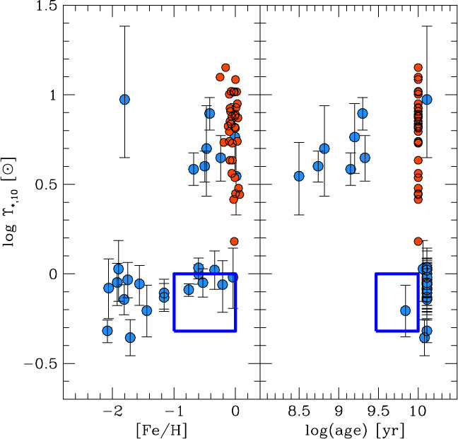
Figure 2. The stellar mass-to-light ratio at 10 Gyr, ϒ*,10, as a function of metallicity and age, showing two distinct populations. Clusters (blue data points) with younger ages, or higher metallicities, tend to show higher mass-to-light ratios, indicative of an IMF similar to Salpeter (α = −2.35) over the full mass range. Older, more metal-poor, clusters have mass-to-light ratios consistent with an IMF having proportionally fewer low-mass stars, such as that of Kroupa et al. (Reference Kroupa, Tout and Gilmore1993). The red data points represent the mass-to-light ratios for early-type galaxies, while the blue box indicates the range of ϒ*,10 for disk galaxies. See Zaritsky et al. (Reference Zaritsky, Colucci, Pessev, Bernstein and Chandar2014b) for details. (Figure 9 of ‘Evidence for two distinct stellar initial mass functions: Probing for clues to the dichotomy’, Zaritsky et al. (Reference Zaritsky, Colucci, Pessev, Bernstein and Chandar2014b), © AAS. Reproduced with permission.)
3.2. Stellar clusters
In their review of the formation of young massive clusters, Portegies Zwart et al. (Reference Portegies Zwart, McMillan and Gieles2010) conclude by noting that ‘globular clusters are simply old massive clusters, the logical descendants of young massive clusters in the early Universe’, a view supported by Kruijssen (Reference Kruijssen2015). Zaritsky et al. (Reference Zaritsky, Colucci, Pessev, Bernstein and Chandar2012, Reference Zaritsky, Colucci, Pessev, Bernstein and Chandar2013, Reference Zaritsky, Colucci, Pessev, Bernstein and Chandar2014b) use the stellar mass-to-light ratios in Milky Way and Local Group stellar and globular clusters to infer, in contrast to the results above, two distinct stellar IMFs in such systems, which they describe as a ‘bimodal’ IMF (Figure 2).
This result was initially established by measuring the stellar mass-to-light ratio in the V-band, ϒ*, based on observed velocity dispersions of four key clusters (Zaritsky et al. Reference Zaritsky, Colucci, Pessev, Bernstein and Chandar2012), ultimately extended to a sample of 29 clusters among 4 different host galaxies (Zaritsky et al. Reference Zaritsky, Colucci, Pessev, Bernstein and Chandar2014b). The quantity ϒ*,10 was introduced, being the stellar mass-to-light ratio that a cluster would have at the age of 10 Gyr, based on simple evolutionary models, in order to more accurately compare between clusters of different ages. After exploring the impact of stellar binarity on the measured velocity dispersions (Zaritsky et al. Reference Zaritsky, Colucci, Pessev, Bernstein and Chandar2012), and the effects of internal dynamical evolution and relaxation driven mass loss (Zaritsky et al. Reference Zaritsky, Colucci, Pessev, Bernstein and Chandar2013), they conclude that such effects are not enough to account for the observed differences in mass-to-light ratio. The resulting conclusion is that the bimodality seen in ϒ*,10 is evidence for two distinct IMFs, with young stellar clusters (log(t/yr) ≲ 9.5) favouring IMFs similar to Salpeter (α = −2.35) over the full mass range (0.1 < m/M⊙ < 120, Zaritsky et al. Reference Zaritsky, Colucci, Pessev, Bernstein and Chandar2012), with older clusters favouring IMFs similar to that of Kroupa et al. (Reference Kroupa, Tout and Gilmore1993), with proportionally fewer low-mass stars, and a steeper high-mass slope (αh = −2.7). They are careful to note, though, that neither of these IMFs is a unique solution, given that the constraint is on total mass arising from the measured mass-to-light ratios.
There are conflicting results regarding the mass function of globular clusters in the low-mass range (m < 1 M⊙). Using mass-to-light ratios of 200 globular clusters in M31, Strader, Caldwell, & Seth (Reference Strader, Caldwell and Seth2011) find a deficit of low-mass stars compared to a Salpeter slope, with −1.3 < αl < −0.8 for m < 1 M⊙ (although mass underestimates may change this conclusion, see Shanahan & Gieles Reference Shanahan and Gieles2015). Zonoozi, Haghi, & Kroupa (Reference Zonoozi, Haghi and Kroupa2016) argue that an excess of high-mass stars as a function of metallicity can account for the lower than expected mass-to-light ratios of metal-rich globular clusters in M31. van Dokkum & Conroy (Reference van Dokkum and Conroy2011) use stellar absorption features (see Section 5.3) measured for four globular clusters in M31 to infer an IMF consistent with that of Kroupa (Reference Kroupa2001), with no low-mass excess. In contrast, Goudfrooij & Kruijssen (Reference Goudfrooij and Kruijssen2014) show that some globular cluster systems (at least the metal-rich population) in elliptical galaxies have a low-mass excess, requiring −3.0 < αl < −2.3 over 0.3 < m/M⊙ < 0.8. Zaritsky et al. (Reference Zaritsky, Colucci, Pessev, Bernstein and Chandar2014b) go on to show that the high and low mass-to-light ratios for their stellar clusters are well matched to those of early- and late-type galaxies, respectively (Figure 2), and potentially also consistent with the variations in IMF proposed for such systems (e.g. Gunawardhana et al. Reference Gunawardhana2011; van Dokkum & Conroy Reference van Dokkum and Conroy2012). This suggests an observational approach that can be used for directly linking and comparing studies of stellar and galactic systems.
Accounting for dynamical evolution is important in understanding how the observed mass function of a star cluster changes with time and may be related to its IMF. Some simulations demonstrate that the impact of tidal fields on star clusters, or that gas expulsion from initially mass segregated globular clusters, ejects predominantly low-mass stars (e.g. Baumgardt & Makino Reference Baumgardt and Makino2003; Haghi et al. Reference Haghi, Zonoozi, Kroupa, Banerjee and Baumgardt2015). Others demonstrate the mechanisms by which star clusters can eject high-mass stars (e.g. Oh & Kroupa Reference Oh and Kroupa2016; Banerjee & Kroupa Reference Banerjee and Kroupa2012). It is clear that there are many subtleties and details that need to be considered carefully in inferring an IMF from complex dynamically and astrophysically evolving systems.
The challenges in measuring star counts and accounting for mass segregation in star clusters when investigating the high-mass end of the IMF can be sidestepped through measuring the hydrogen ionising photon rate (Calzetti et al. Reference Calzetti, Chandar, Lee, Elmegreen, Kennicutt and Whitmore2010; Andrews et al. Reference Andrews2013, Reference Andrews2014). Andrews et al. (Reference Andrews2014) demonstrate the presence of high-mass stars in young (t < 8 Myr) low-mass clusters (down to cluster masses of M cl ≈ 500 M⊙) in M83. They conclude that star clusters are populated stochastically, or randomly, in stellar mass, allowing the existence of high-mass stars (up to 120 M⊙) even in the lowest mass clusters (M cl ≈ 500 M⊙), in direct contrast with the mu − M cl relation of Weidner, Kroupa, & Bonnell (Reference Weidner, Kroupa and Bonnell2010) (but see also Weidner, Kroupa, & Pflamm-Altenburg Reference Weidner, Kroupa and Pflamm-Altenburg2014). They conclude that the population of M83 star clusters they observe have a total Hα luminosity to cluster mass ratio consistent with that expected from a Kroupa (Reference Kroupa2001) IMF with 0.08 < m/M⊙ < 120.
Also exploring star clusters in a nearby galaxy, Weisz et al. (Reference Weisz2015) have undertaken a large systematic study of the colour-magnitude diagrams for 85 young, intermediate mass stellar clusters in M31. Using a framework to infer the distribution of mass function slopes given a set of noisy measurements (Hogg, Myers, & Bovy Reference Hogg, Myers and Bovy2010; Foreman-Mackey, Hogg, & Morton Reference Foreman-Mackey, Hogg and Morton2014), they find that the high-mass slope of the IMF is best described by  $ {\alpha _h} = - 2.45_{ - 0.03}^{ + 0.06} $, somewhat steeper than the high-mass slope of Kroupa (Reference Kroupa2001) (αh = −2.3) inferred by Andrews et al. (Reference Andrews2014). This is similar to the result of Veltchev, Nedialkov, & Borisov (Reference Veltchev, Nedialkov and Borisov2004) who found αh = −2.59 ± 0.09 (for m ≳ 7 M⊙) using colour-magnitude diagrams for 50 OB associations in the south-western region of M31.
The conclusions of Andrews et al. (Reference Andrews2014) and Weisz et al. (Reference Weisz2015) reveal part of the challenge in discussing and understanding the IMF. Both Andrews et al. (Reference Andrews2014) and Weisz et al. (Reference Weisz2015) present their results as being consistent with a ‘universal’ IMF. The claim is that the IMF for the population of clusters as a whole produces an IMF consistent with that measured for the Milky Way, although the individual clusters demonstrate observed ‘variations’. Any of the individual low-mass star clusters of Andrews et al. (Reference Andrews2014), for example, that contain a very high-mass star will necessarily demonstrate an IMF skewed to the high-mass end, and be different to the IMF of other clusters in the M83 ensemble, even though their ensemble IMF is consistent with that of Kroupa (Reference Kroupa2001). Equally, the M31 cluster IMF slopes found by Weisz et al. (Reference Weisz2015) show significant scatter individually (see their Figure 4), while the ensemble is well described by IMFs having high-mass slopes drawn from a normal distribution with a very narrow intrinsic dispersion.
What the results of Andrews et al. (Reference Andrews2014) demonstrate, but which is not made explicit, is that stochastic or random sampling of the IMF for a given cluster leads directly to variations in the IMF between clusters. The importance of stochasticity in the IMF is also highlighted by Barker, de Grijs, & Cerviño (Reference Barker, de Grijs and Cerviño2008). The ambiguity here is deeply buried in the difference between a ‘universal’ process of star formation compared to a ‘universal’ mass distribution produced from any given star formation event, a complication that has led to an entire industry exploring how the IMF is populated (see, e.g. discussion in Kroupa et al. Reference Kroupa, Weidner, Pflamm-Altenburg, Thies, Dabringhausen, Marks and Maschberger2013). The conclusions of Andrews et al. (Reference Andrews2014) and Weisz et al. (Reference Weisz2015) are in support of the former (a ‘universal’ process), but not the latter. Given these consistent conclusions, the small but measurable difference in αh between M31 (Weisz et al. Reference Weisz2015) and M83 (Andrews et al. Reference Andrews2014) is worth noting. Both cases here also highlight the difference between an IMF inferred for any individual star cluster and that for a galaxy taken as a whole, a distinction that will be a recurring theme in this review.
While Weisz et al. (Reference Weisz2015) also use their technique to show αh = −2.15 ± 0.1 for the Milky Way and αh = −2.3 ± 0.1 for the LMC, they argue that to be robust these values would need to be calculated using the same homogeneous and principled approach as they applied to M31. They go on to recommend that their steeper  $ {\alpha _h} = - 2.45_{ - 0.03}^{ + 0.06} $ slope for m > 1 M⊙ be used in the ‘universal’ IMF shape. When calculating SFRs this IMF slope leads to values 30–50% higher than assuming the Kroupa (Reference Kroupa2001) IMF. I return to this point in Section 6.
Other observations of starburst clusters and super star clusters provide conflicting evidence for the shape of the IMF. Such systems, containing numerous and unresolved stellar components, have been investigated using a range of techniques, including spectroscopic observations, in some cases analysed using SPS models, mass-to-light ratios, and dynamics. A deficit of low-mass stars has been identified in the super star cluster M82F within the galaxy M82 (Smith & Gallagher Reference Smith and Gallagher2001; McCrady, Graham, & Vacca Reference McCrady, Graham and Vacca2005; Bastian et al. Reference Bastian, Konstantopoulos, Smith, Trancho, Westmoquette and Gallagher2007). The impact of a deficit of low-mass stars on the dynamical evolution of such clusters appears relatively mild (Kouwenhoven et al. Reference Kouwenhoven, Goodwin, de Grijs, Rose and Kim2014). The Milky Way’s nuclear star cluster was analysed by Lu et al. (Reference Lu, Do, Ghez, Morris, Yelda and Matthews2013), who find an IMF slope of αh = −1.7 (for 1 < m/M⊙ < 150) and an age of around 3.3 Myr. There is evidence for a Salpeter IMF (α = −2.35 for the full mass range 0.1 < m/M⊙ < 100) in a massive young cluster in the Antennae (Greissl et al. Reference Greissl, Meyer, Christopher and Scoville2010), which would imply an excess of low-mass stars relative to a Kroupa (Reference Kroupa2001) or Chabrier (Reference Chabrier2003a) IMF, but other dynamical mass estimates suggest ‘standard Kroupa IMFs’ (although without detailing whichFootnote e) in star clusters in the Antennae and NGC 1487 (Mengel et al. Reference Mengel, Lehnert, Thatte, Vacca, Whitmore and Chandar2008). Banerjee & Kroupa (Reference Banerjee and Kroupa2012) use simulations to argue that the true IMF of R136 must have had an excess of high-mass stars, given that their dynamical ejection is efficient, and that the observed mass function is consistent with that of Kroupa (Reference Kroupa2001). The early suggestions of a high value for ml in starburst nuclei (e.g. Rieke et al. Reference Rieke, Lebofsky, Thompson, Low and Tokunaga1980) have not been supported by more recent work, with Rigby & Rieke (Reference Rigby and Rieke2004) finding evidence using mid-infrared Ne line ratios for either mc ≈ 40 M⊙ (or equivalently a strong steepening in the high-mass IMF slope above this value), or that high-mass stars in starbursts are embedded within ultra-compact Hii regions, preventing the nebular lines from forming and escaping, the solution they favour (see also summaries by Elmegreen Reference Elmegreen, de Grijs and González Delgado2005, Reference Elmegreen, Kang, Lee, Leung and Cheng2007). Recent results analysing the 30 Doradus star forming region in the LMC (Schneider et al. Reference Schneider2018) show strong evidence for an IMF well populated up to mu ≈ 200 M⊙, and with 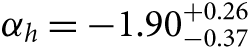 $ {\alpha _h} = - 1.90_{ - 0.37}^{ + 0.26} $ for 15 < m/M⊙ < 200. Taken together, such results appear to provide evidence for a relative excess of high-mass stars in some, but not all, starburst clusters.
3.3. Chemical abundance measurements
Another common stellar technique used in inferring an IMF relies on the chemical abundances of stars. Since different elements are produced by stars of different mass, the present-day elemental abundances can be used to infer an indirect measure of the IMF. The summary by Wyse (Reference Wyse, Gilmore and Howell1998) provides an excellent overview of this approach and its issues and limitations. Broadly, oxygen and the α-elements are produced predominantly in core-collapse (Type II) supernovae, while iron is produced in both core-collapse and thermonuclear (Type Ia) supernovae. The ratio of [O/Fe] can then be used to probe the high-mass star IMF, with a ‘plateau’ in this ratio arising from stars pre-enriched only by type-II SNe, the quantitative value of which would change with a change in the high-mass IMF slope. A limitation is that the value of this type-II plateau depends on the theoretical yields assumed for different elements as a function of supernova progenitor mass. Wyse & Gilmore (Reference Wyse and Gilmore1992) note that varying the IMF slope from αh = −2.1 to αh = −3.3 (for m > 1 M⊙) results in [O/Fe] changing by ≈ 0.4 dex, although the difference for the smaller range of −2.5 < αh < −2.1 is only Δ[O/Fe] ≈ 0.1 – 0.15 dex depending on the elemental yields assumed (their Tables 1 and 2). Wyse (Reference Wyse, Gilmore and Howell1998) argues that for the Milky Way stellar halo, thick disk, and bulge populations, the measured abundances are consistent with a Salpeter high-mass IMF slope. A compilation of abundances was used by Nicholls et al. (Reference Nicholls, Sutherland, Dopita, Kewley and Groves2017) in introducing a new approach to scaling abundances with total metallicity, reinforcing the detection of the type-II plateau for the Milky Way, LMC, and the Sculptor Dwarf (shown using [Mg/Fe], Nicholls et al. (Reference Nicholls, Sutherland, Dopita, Kewley and Groves2017, Figure 9)).
Combining abundance constraints with mass-to-light ratio constraints, Tsujimoto et al. (Reference Tsujimoto, Yoshii, Nomoto, Matteucci, Thielemann and Hashimoto1997) find −2.6 < αh < −2.3 for m > 1 M⊙ for stars presently in the solar neighbourhood. They also argue for mu = 50 ± 10 M⊙, although this mu is not necessarily the highest mass of stars formed, but instead is the highest mass of stars that return chemically enriched material to the interstellar medium. In their analysis stars may exist above this mass, but those that do must end as black holes without ejecting processed material into the interstellar medium. This result has been called into question by Gibson (Reference Gibson1998), though, who demonstrates that using different chemical yield models relaxes this outcome to a much less stringent constraint of mu ≈ 30 – 200 M⊙.
The chemical abundances of stars in some dwarf spheroidal (dSph) satellites of the Milky Way show measurable differences from Milky Way stars. Early work suggested that any abundance differences were still consistent with an IMF having a Salpeter high-mass slope (e.g. Tolstoy et al. Reference Tolstoy, Venn, Shetrone, Primas, Hill, Kaufer and Szeifert2003; Venn et al. Reference Venn, Irwin, Shetrone, Tout, Hill and Tolstoy2004). A high-mass truncation of the IMF was discussed as a possible scenario to explain the differences, but a solution arising from the contributions of metal-poor AGB stars was favoured. More recently, Tsujimoto (Reference Tsujimoto2011) argue that the deficiency of α-elements combined with an enhancement in s-process elements (Ba) found in dSph galaxies provides evidence of a lack of high-mass stars (m ≳ 25 M⊙) in these systems, a result in keeping with the idea of a lower value for mu in lower SFR environments (Weidner & Kroupa Reference Weidner and Kroupa2005). This result is supported by a different type of constraint, explored by Portinari et al. (Reference Portinari, Sommer-Larsen and Tantalo2004a), who find that IMFs typical of the Milky Way (Kennicutt Reference Kennicutt1983; Larson Reference Larson1998; Chabrier Reference Chabrier2001) can explain the mass-to-light ratios seen in Sbc/Sc galaxies but then overestimate the metallicities. They argue that unless the observed metallicity is underestimated (due to expulsion into the intergalactic medium or through being locked up in dust grains), the IMF needs to be truncated at high masses. This result was extended by Portinari et al. (Reference Portinari, Moretti, Chiosi and Sommer-Larsen2004b), showing that a ‘standard solar neighbourhood IMF’ (Kroupa Reference Kroupa, Rebolo, Martin and Zapatero Osorio1998) cannot provide sufficient heavy elements to account for the observed metallicity of galaxies in clusters. None of these analyses account for galactic winds, which, if included, may help explain the observed chemical signatures without the need for the lower value of mu, although Portinari et al. (Reference Portinari, Moretti, Chiosi and Sommer-Larsen2004b) note that this would require ‘substantial loss of metals from the solar neighbourhood and from disk galaxies in general’.
At the other extreme, a recent analysis of starburst galaxies by Romano et al. (Reference Romano, Matteucci, Zhang, Papadopoulos and Ivison2017), using updated chemical models to track CNO isotopes and accounting for stellar rotation, finds a need for an excess of high-mass stars (αh = −1.95 for m > 0.5 M⊙) to reproduce observed isotope abundances. This result is consistent with the conclusions of Sliwa et al. (Reference Sliwa, Wilson, Aalto and Privon2017) who find a need for an excess of high-mass stars to explain the CO isotopic abundances in the starburst galaxy IRAS 13120-5453.
A related approach links the cosmic microwave background (CMB) to a directly observable stellar chemical signature, the carbon-enhanced metal-poor (CEMP) stars (Tumlinson Reference Tumlinson2007), probing stars in the mass range 1 < m/M⊙ < 8. The CMB defines a temperature minimum that may translate to a characteristic fragmentation scale for star-forming gas (Larson Reference Larson2005). The time dependence of the CMB can hence have an impact on the fraction of CEMP stars as a function of metallicity, and Tumlinson (Reference Tumlinson2007) found that mc should increase towards higher redshift. This result is supported by analyses of observed CEMP stars (Komiya et al. Reference Komiya, Suda, Minaguchi, Shigeyama, Aoki and Fujimoto2007) explained as arising from binary systems, and as modelled by binary population synthesis (Suda et al. Reference Suda2013). Tumlinson (Reference Tumlinson2007) pointed out that such an evolution of the IMF would lead to two clear systematic errors if it is not accounted for. Early-time SFHs for local galaxies derived from colour-magnitude diagrams assuming a non-evolving IMF would be systematically underestimated, and SFRs from high-z luminosity tracers, such as UV, would be systematically overestimated. I return to these points in Section 6.
While constraints from stellar chemistry in this fashion may turn out to be quite powerful probes of the IMF, in particular its properties at high redshift, it would be valuable to explore how limitations or systematics in our understanding of stellar yields and binary star evolution may influence or limit such measurements. One of the important potential advantages of stellar chemistry, and in particular the most metal-poor stars, is their potential for probing the first generation of stars, called ‘Population III’ stars (Frebel Reference Frebel2010), through the preserved signatures of their supernova chemical yields in subsequent generations of stars. I briefly discuss this in the next section.
3.4. Population III stars
Simulations and physical arguments have demonstrated for many years that Population III stars are likely to be dominated by high-mass objects (e.g. Abel, Bryan, & Norman Reference Abel, Bryan and Norman2002; Bromm, Coppi, & Larson Reference Bromm, Coppi and Larson2002), with typical masses m > 100 M⊙ and few or no low-mass stars (see review by Bromm & Larson Reference Bromm and Larson2004, and references therein). Further work has explored the impact of such Population III star properties for the earliest generations of galaxies (Bromm & Yoshida Reference Bromm and Yoshida2011). The physical processes involved are also summarised well, in the broader context of structure formation and evolution, by Loeb (Reference Loeb2006). More recently, some simulations now appear to extend the lower mass limit for Population III stars to lower values (e.g. Hirano et al. Reference Hirano, Hosokawa, Yoshida, Umeda, Omukai, Chiaki and Yorke2014; Susa, Hasegawa, & Tominaga Reference Susa, Hasegawa and Tominaga2014). Clearly the IMF for such a population would be radically different to that in the local Universe and in that sense there is trivially an evolution in the IMF. This does not address the question that is usually meant regarding the ‘universality’ of the IMF, though, which instead is focused on whether the IMF may be different between coeval galaxies, or between different star-forming regions within a galaxy. With that in mind, it is instructive to briefly touch on some of the results associated with the current measurements probing Population III stars.
Observational probes of the first stars are summarised in the review by Bromm & Larson (Reference Bromm and Larson2004), who highlight their reionisation signature, chemical enrichment of subsequent stellar generations (stellar archaeology), and gamma-ray bursts as opportunities then developing. This builds on a significant body of earlier work to explore and explain the lack of low metallicity stars in the Milky Way and its halo (e.g. Bond Reference Bond1981; Jones Reference Jones1985; Cayrel Reference Cayrel1986) and other novel probes of Population III stars (e.g. Tarbet & Rowan-Robinson Reference Tarbet and Rowan-Robinson1982). Subsequently, gamma-ray bursts have been used to constrain the high-z SFH (Yüksel et al. Reference Bertelli Motta, Clark, Glover, Klessen and Pasquali2008; Kistler et al. Reference Kistler, Yüksel, Beacom, Hopkins and Wyithe2009; Kistler, Yuksel, & Hopkins Reference Kistler, Yüksel, Beacom, Hopkins and Wyithe2013), finding a higher value of the SFR density for z > 5 than commonly inferred from deep imaging data (see summary in Madau & Dickinson Reference Madau and Dickinson2014), with implications for reionisation (Wyithe et al. Reference Wyithe, Hopkins, Kistler, Yüksel and Beacom2010), although with no direct constraints yet on the Population III IMF. Ma et al. (Reference Ma, Maio, Ciardi and Salvaterra2015) show that none of the gamma-ray bursts detected at 5 ≲ z ≲ 6 show abundance ratios consistent with an environment dominated by Population III stars. Opportunities for probing the first stars through stellar archaeology are summarised by Frebel (Reference Frebel2010) and in an extensive review by Karlsson, Bromm, & Bland-Hawthorn (Reference Karlsson, Bromm and Bland-Hawthorn2013). Strong abundance ratio signatures are expected, with Heger & Woosley (Reference Heger and Woosley2010), for example, demonstrating that increasing ml from 10 to 40 M⊙ strongly suppresses the production of elements heavier than aluminium.
Other observations are now starting to constrain the possible IMF shapes for this earliest generation of stars. Sobral et al. (Reference Sobral, Matthee, Darvish, Schaerer, Mobasher, Röttgering, Santos and Hemmati2015) argue for a ‘flat or top-heavy IMF’ (lacking stars below 10 M⊙) for Population III stars in a high-redshift (z = 6.6) Lyα system, although Bowler et al. (Reference Bowler, McLure, Dunlop, McLeod, Stanway, Eldridge and Jarvis2017) dispute this conclusion based on deeper infrared observations. They argue for a low-mass narrow-line active galactic nucleus (AGN) or low metallicity starburst to explain the observed infrared colours. Fraser et al. (Reference Fraser, Casey, Gilmore, Heger and Chan2017) use abundances in extremely metal-poor stars to infer a Salpeter IMF slope, 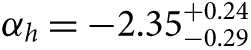 $ {\alpha _h} = - 2.35_{ - 0.29}^{ + 0.24} $, with a maximum supernova progenitor mass of $ m = 87_{ - 33}^{ + 13}{\kern 1pt} {{\rm{M}}_ \odot } $ and a value of ml below the minimum mass for Population III supernovae (ml ≲ 9 M⊙). Hartwig et al. (Reference Hartwig, Bromm, Klessen and Glover2015) demonstrate a technique for constraining the lower mass limit of Population III stars, finding that they can exclude stars with m < 0.65 M⊙ at 95% confidence.
Future observations hold great promise for constraining the high-z IMF. Using simulations, de Souza et al. (Reference de Souza, Ishida, Whalen, Johnson and Ferrara2014) show that a few hundred supernovae detections with the JWST could be sufficient to discriminate between a ‘Salpeter and flat mass distribution for high-redshift stars’. Jeřábková et al. (Reference Jeřábková, Kroupa, Dabringhausen, Hilker and Bekki2017) demonstrate the redshift-dependent photometric properties of globular clusters and ultra-compact dwarf galaxies to provide observable IMF diagnostics for anticipated JWST observations.
With this review focused primarily on the consistency of approaches to observational constraints of the IMF I do not discuss Population III stars further. It is clear that this area will see rapid growth of a variety of observational constraints in the near future, and I hope that the framework presented here will be applied to these approaches to aid in understanding this earliest generation of stars.
3.5. Review
With the broad range of approaches, techniques, and results described above, it is worth briefly summarising. Star clusters sample physical scales on the order of a few pc and a broad range of ages and SFRs, although most of those observed are high SFR surface density objects. The field star population in principle probes the full galaxy-wide scale (tens of kpc) and is sensitive to the galaxy-wide SFH.
Although the large uncertainties and systematics involved in these measurements understandably lead to a conclusion that the IMFs are all similar and broadly consistent with (e.g.) the IMFs of Kroupa (Reference Kroupa2001) or Chabrier (Reference Chabrier2003a), it is tantalising to note that the field star and stellar association population have high-mass (m > 1 M⊙) slopes on average somewhat steeper (αh ≈ −2.5) than the cluster stars (αh ≈ −2.2, see Figure 2 in Bastian et al. Reference Bastian, Covey and Meyer2010). The populations of globular clusters and extragalactic star clusters, in contrast, show evidence for some differences between IMFs. Probing spatial scales on the order of pc, a range of IMFs are inferred, with some globular clusters consistent with the IMF of Kroupa et al. (Reference Kroupa, Tout and Gilmore1993) and its steeper high-mass slope (αh = −2.7), and others consistent with a Salpeter slope over the full mass range extending to the lowest masses. It is worth noting the link between the mass-to-light ratio approaches for globular clusters and galaxy systems as a technique that may lend itself to being applied self-consistently across a broad range of different physical scales and conditions.
Extragalactic star clusters demonstrate IMFs consistent with Kroupa (Reference Kroupa2001) in M83 (αh = −2.3), or with high-mass slopes somewhat steeper (αh = −2.45) in M31. While this difference is small, the level of precision of these results begins to suggest that it is not negligible. At least some starburst and super star clusters tend to show evidence for an excess of high-mass stars, either through an increase in mc or a flatter αh compared to the IMF of Kroupa (Reference Kroupa2001). Approaches using abundance measurements reinforce the slightly steeper high-mass slope seen in field stars and further suggest the possibility that the high-mass limit mu may need to be somewhat lower than the typical Milky Way value in nearby dSph galaxies.
Taken as a whole, while the range of uncertainties and systematics makes it easy to assert that there is no strong evidence measured for IMF variations, adopting the converse approach of placing constraints on the scale of possible variations opens a different line of argument. Referring below to the Kroupa (Reference Kroupa2001) or Chabrier (Reference Chabrier2003a) IMF as the ‘typical’ IMF for the Milky Way, it can be said that:
For stars and star clusters within Local Group galaxies, the high-mass IMF slope does not vary more than ±0.3 around αh = −2.5.
For extragalactic globular clusters, there are conflicting observations of mass-to-light ratios, which are parameterised as a constraint on the low-mass (m < 1 M⊙) slope ranging across −3.0 < αl < −0.8, from a deficit to an excess compared to the typical Milky Way values.
In high SFR regions (starburst or super star clusters), there is an apparent variation with some having mc ≳ 1 M⊙ or αh > −2.3, higher than the typical values in the Milky Way.
In low SFR regions (dSph galaxies), there may be an apparent variation with mu needing to be somewhat lower than the typical value in the Milky Way.
It is worth recalling here that there may be degeneracies between mu and αh, and that the measured constraints may be able to be reproduced by different parameter combinations. It remains the case, though, that there does appear to be some difference between the form of the IMF in high and low SFR regions. These lines of evidence suggest that the IMF is not ‘universal’, but that there are differences in different regions, although the details are only qualitatively constrained.
4. IMF measurement approaches: neutral and molecular gas and dust
It is natural when investigating the IMF to turn from already existing stars to the progenitor clouds in which they form, to probe the earliest stages of the formation process. This is explored most efficiently through measurements of cold gas and dust in molecular clouds. Due to observational practicalities, much of the work here has focused on clouds within the Milky Way and nearby galaxies and is well summarised in reviews by Zinnecker & Yorke (Reference Zinnecker and Yorke2007), Tan et al. (Reference Tan, Beltrán, Caselli, Fontani, Fuente, Krumholz, McKee and Stolte2014), and Offner et al. (Reference Offner, Clark, Hennebelle, Bastian, Bate, Hopkins, Moraux and Whitworth2014). There is ample evidence demonstrating that the mass function for the molecular ‘cores’ (those gas regions of sufficient density to go on to form stars) has a similar shape to the stellar IMF in the Milky Way (e.g. André et al. Reference André2010; Könyves et al. Reference Könyves2010; Montillaud et al. Reference Montillaud2015; Marsh et al. Reference Marsh2016a). Many core mass functions (CMFs) show an offset in mass compared to the IMFs of Kroupa (Reference Kroupa2001) or Chabrier (Reference Chabrier2003a), with the break in the power law at masses larger by a factor of ≈ 3 – 4, and with a similar range of variations in the high-mass slope between different molecular clouds as seen in the various stellar analyses (see summary by Offner et al. Reference Offner, Clark, Hennebelle, Bastian, Bate, Hopkins, Moraux and Whitworth2014). Despite the range of variations, such results have for decades been similarly interpreted as consistent with a ‘universal’ form and have led naturally to the idea that the CMF and IMF are linked physically through some star formation efficiency factor.
The connection between pre-stellar CMFs and the IMF is still not clear, although many models have been proposed to explain it (e.g. Hopkins Reference Hopkins2013b; Guszejnov & Hopkins Reference Guszejnov and Hopkins2015; Zhou et al. Reference Zhou, Huang, Lin, Gritschneder and Lau2015). One issue is how a core is defined observationally, and that observational limitations and different threshold levels for defining a core lead to different results (see discussions by, e.g. Elmegreen Reference Elmegreen2009; Offner et al. Reference Offner, Clark, Hennebelle, Bastian, Bate, Hopkins, Moraux and Whitworth2014). As noted by Offner et al. (Reference Offner, Clark, Hennebelle, Bastian, Bate, Hopkins, Moraux and Whitworth2014), ‘Different algorithms … even when applied to the same observations, do not always identify the same cores, and when they do, they sometimes assign widely different masses’. Even if cores can be adequately identified, there is evidence questioning the fragmentation models leading from cores to stars, and hence linking the IMFs of each (Holman et al. Reference Holman, Walch, Goodwin and Whitworth2013; Bertelli Motta et al. Reference Bertelli Motta, Clark, Glover, Klessen and Pasquali2016).
A more robust approach than discrete core identifications is to use the full probability distribution function (PDF) of observed column densities within a star-forming cloud, in order to identify which regions may have sufficient density to be star forming (e.g. Rathborne et al. Reference Rathborne2014). There is an open question over whether there exists some threshold in column density of molecular hydrogen above which star formation proceeds efficiently. A universal threshold of N(H 2) ≳ 1.4 × 1022 cm2 was proposed by Lada et al. (Reference Lada, Forbrich, Lombardi and Alves2012), although Krumholz, Dekel, & McKee (Reference Krumholz, Dekel and McKee2012) argue against the existence of such a threshold. At least one counterexample, the Galactic centre molecular cloud G0.253 + 0.016, questions the idea of a universal threshold (Rathborne et al. Reference Rathborne2015). Dust temperature measurements of this cloud suggest that star formation may have recently begun, with detection of a cool filament whose hot central region is undergoing gravitational collapse and fragmentation to form a ‘line of protostars’ (Marsh et al. Reference Marsh, Ragan, Whitworth and Clark2016b). Despite this, the central molecular zone of the Milky Way appears to support substantially less star formation than might be expected from a column density threshold (Longmore et al. Reference Longmore2013). These results bring the idea of a universal threshold into question, at least for environments with the extreme high pressures found in the Milky Way central molecular zone, which may mimic the conditions of star formation at high redshift.
Broadly, the studies of pre-stellar clouds suggest that turbulence and hierarchical fragmentation are dominant processes in driving the star formation. Turbulence as a dominant contributor to the star formation process has also been shown to be effective in high pressure environments (Rathborne et al. Reference Rathborne2014), and may therefore be significant in starburst nuclei and high redshift galaxies. High-mass stars and clusters can form in filamentary molecular clouds (Contreras et al. Reference Contreras, Garay, Rathborne and Sanhueza2016), although Contreras et al. (Reference Contreras, Rathborne, Guzman, Jackson, Whitaker, Sanhueza and Foster2017) note that high-mass protoclusters are very rare in the Galaxy. Young high-mass clusters in the Milky Way have been shown to form hierarchically rather than through monolithic collapse (Walker et al. Reference Walker, Longmore, Bastian, Kruijssen, Rathborne, Jackson, Foster and Contreras2015), a result seen also in the arms of the grand-design spiral NGC 1566, where Gouliermis et al. (Reference Gouliermis2017) demonstrate hierarchical star formation driven by turbulence. Grasha et al. (Reference Grasha2017) show that star cluster formation in eight local galaxies is hierarchical both in space and time, and that the ages of adjacent clusters are consistent with turbulence driving the star formation. In contrast, there is evidence for monolithic collapse in the formation of some young Galactic star clusters (e.g. Banerjee & Kroupa Reference Banerjee and Kroupa2014, Reference Banerjee and Kroupa2015, Reference Banerjee, Kroupa and Stahler2018).
Turbulence alone, though, does not seem to be a sufficient mechanism. Using high resolution observations of molecular gas in M51, Leroy et al. (Reference Leroy2017) note that observed measures of star formation efficiency are in some tension with turbulent star-formation models, finding an anticorrelation between the star formation efficiency per free-fall time with the surface density and line width of molecular gas. Vutisalchavakul, Evans, & Heyer (Reference Vutisalchavakul, Evans and Heyer2016), based on star-forming regions in the Galactic plane, argue that observed relations between SFR and molecular cloud properties are inconsistent with those seen in extragalactic relations or the model by Krumholz et al. (Reference Krumholz, Dekel and McKee2012). Similarly, Heyer et al. (Reference Heyer, Gutermuth, Urquhart, Csengeri, Wienen, Leurini, Menten and Wyrowski2016) find low values of star formation efficiency per free-fall time in a sample of Galactic young stellar objects, noting that the strongest correlations of SFR surface density are with the dense gas surface density normalised by the free-fall and clump crossing times. They state that models accounting for such local gas conditions provide a reasonable description of these observations. Lee, Miville-Deschênes, & Murray (Reference Lee, Miville-Deschênes and Murray2016) find a rather higher observed scatter in star formation efficiency for star-forming giant molecular clouds in the Milky Way, which they also note is unable to be explained by constant (Krumholz & McKee Reference Krumholz and McKee2005) or turbulence-related (Hennebelle & Chabrier Reference Hennebelle, Chabrier, Alves, Elmegreen, Girart and Trimble2011) star formation. They argue instead for a time-variable rate of star formation noting that ‘sporadic small-scale star formation will tend to produce more massive clusters than will steady small-scale star formation’. By analysing the dense gas in star-forming clusters, Hacar, Tafalla, & Alves (Reference Hacar, Tafalla and Alves2017) argue that both clustered and non-clustered star-forming regions might be naturally explained through the spatial density of dense gas ‘sonic fibres’ (Hacar et al. Reference Hacar, Tafalla, Kauffmann and Kovács2013). Hacar et al. (Reference Hacar, Tafalla, Forbrich, Alves, Meingast, Grossschedl and Teixeira2018) extends this approach to propose a unified star formation scenario that leads naturally to the observed differences between low and high-mass clouds, and the origin of clusters. Walker et al. (Reference Walker, Longmore, Bastian, Kruijssen, Rathborne, Galván-Madrid and Liu2016) show that the mass surface density profiles are shallower for gas clouds than for young massive star clusters in the Milky Way. They argue that this implies an evolution requiring mass to continue to accumulate towards cloud centres in highly star-forming clouds after the onset of star formation, in a ‘conveyor-belt’ scenario.
It is beyond the scope of this review to explore in-depth the range of detailed models of star formation, and their strengths and limitations. Summaries, however, of some models describing the star formation process and linking the CMF to the IMF, or that aim to explain the IMF shape, are presented in Section 7. A detailed review of the formation of young high-mass star clusters is given by Portegies Zwart et al. (Reference Portegies Zwart, McMillan and Gieles2010), and Tan et al. (Reference Tan, Beltrán, Caselli, Fontani, Fuente, Krumholz, McKee and Stolte2014) provide a thorough review of high-mass star formation. Interestingly, Zinnecker & Yorke (Reference Zinnecker and Yorke2007) find strong support for an IMF upper mass limit of mu ≈ 150 M⊙ and make the case that high-mass star formation proceeds differently from low-mass star formation, not just as a scaled-up version, but ‘partly a mechanism of its own, primarily owing to the role of stellar mass and radiation pressure in controlling the dynamics’. This conclusion has been questioned by more recent work, summarised by Tan et al. (Reference Tan, Beltrán, Caselli, Fontani, Fuente, Krumholz, McKee and Stolte2014), who argue that most observations support a common mechanism for star formation from low to high masses.
A different approach linking star-forming gas to the IMF was used by Hopkins, McClure-Griffiths, & Gaensler (Reference Hopkins and Beacom2008) to explore the link between gas consumption and star formation in a cosmic global average sense. They use the Kennicutt–Schmidt law linking SFR and gas surface densities, following Hopkins, Rao, & Turnshek (Reference Hopkins, Rao and Turnshek2005) who convert such a surface density relation to a volume density relation using the observed redshift distributions of damped Lyman α absorbers. The IMF dependency arises through the SFR density measurement. Different assumed IMFs will alter the SFR density calculated from observed luminosity densities, and consequently the corresponding volume density of gas necessary to sustain such star formation levels. Hopkins et al. (Reference Hopkins, McClure-Griffiths and Gaensler2008) infer that the cosmic mass density of HI at high redshift (z > 1) implies SFR densities that are not consistent with an IMF typical of the Milky Way such as Kroupa (Reference Kroupa2001) or Chabrier (Reference Chabrier2003a). Instead, they require an IMF with a high-mass slope flatter than Salpeter (αh > –2.35), such as that proposed through the evolving IMF of Wilkins et al. (Reference Wilkins, Trentham and Hopkins2008a). It would be valuable to revisit this alternative style of approach in light of more recent work on the relationship between SFR and gas density, as reviewed, for example, by Kennicutt & Evans (Reference Kennicutt and Evans2012).
In summary, as with the stellar techniques, the approaches used in measuring the CMF in order to link it to the IMF are limited by the relatively small samples available within the Milky Way and nearby galaxies, and the link itself may be unclear (Holman et al. Reference Holman, Walch, Goodwin and Whitworth2013; Bertelli Motta et al. Reference Bertelli Motta, Clark, Glover, Klessen and Pasquali2016). As with the various stellar cluster measurements, a range of CMF high-mass slopes is found for different molecular clouds, with a similar span of uncertainty, and for much the same reason. There are similar levels of variation measured for the low-mass slope and for the characteristic mass where the CMF slope changes. It is worth reiterating the argument of Kruijssen & Longmore (Reference Kruijssen and Longmore2014) regarding the number of independent samples required to capture all phases and the spatial scale of the processes being measured. It is also worth restating and recommending the approach of placing constraints on the scale of possible variations rather than defaulting to a ‘universal’ conclusion.
There is a further point to be made, picking up on the PDF approach of Rathborne et al. (Reference Rathborne2014). They note that gas dense enough to form stars is dense enough to become self-gravitating and undergo runaway collapse. This shows up as a power law tail deviation, at the high column-density end, from the otherwise log-normal form of the PDF. If the gas that will go on to form stars can be identified in this simple and direct way instead, the CMF as an entity, with all the challenges associated in measuring it, is perhaps not a physically useful quantity.
Such a conclusion reinforces the poorly posed nature of the definition of such mass functions. What defines the star-forming region of interest over which the CMF or IMF is to be measured? For gas clouds that have a continuum of densities the challenge in defining boundaries or thresholds (such as with various clump-finding software tools) is clear (e.g. Offner et al. Reference Offner, Clark, Hennebelle, Bastian, Bate, Hopkins, Moraux and Whitworth2014), but the PDF approach sidesteps that limitation. The problem for stars, though, may not be so readily apparent, since for a cluster it would seem straightforward to focus, for example, on the gravitationally bound stars as a single entity. But even this kind of simple scenario has been seen to suffer from issues such as mass segregation, dynamical evolution, and so on, leading to systematics affecting any IMF measurement. This raises the broader concern of whether the IMF itself is a well-posed concept. If it does not exist as a physical distribution at any given point in time (Elmegreen Reference Elmegreen2009; Kroupa et al. Reference Kroupa, Weidner, Pflamm-Altenburg, Thies, Dabringhausen, Marks and Maschberger2013), and the spatial region over which it is to be measured is unclear, is there a better entity that can be more well-defined instead? I return to this point in Section 8.
Having raised again the point regarding the spatial scale being probed, I move next to the approaches used in estimating the IMF for galaxies as a whole.
5. IMF measurement approaches: integrated galaxy techniques
5.1. Background
Techniques for inferring an IMF for a galaxy, as opposed to a star cluster or stellar population, date back to early population synthesis work in the 1960s (Spinrad Reference Spinrad1962; Wood Reference Wood1966; Spinrad Reference Spinrad1966; Spinrad & Taylor Reference Spinrad and Taylor1971) that claimed an excess of M dwarfs in the nuclei of nearby galaxies. Wood (Reference Wood1966) also claim a proportionally larger number of giants for the spiral arms of NGC 224, NGC 3031 (M81), and NGC 5194, ‘essentially identical with that for the Solar neighbourhood’. This approach synthesised galaxy spectra by combining stellar spectra to reproduced the observed galaxy colours and certain spectral features including Mg b and Na D, as well as molecular bands including TiO and CN. These early analyses were focused largely on understanding the stellar populations and explaining the mass-to-light ratio for these systems, rather than constraining the IMF explicitly. Subsequently, Whitford (Reference Whitford1977) showed that the Wing–Ford band was also a sensitive probe of the dwarf-to-giant ratio and demonstrated that it could be used to constrain the IMF for old stellar populations within galaxies. This approach has been revived (e.g. van Dokkum & Conroy Reference van Dokkum and Conroy2012) and is now used routinely to infer IMF properties for early-type galaxies.
A different kind of approach was used by Kennicutt (Reference Kennicutt1983), who introduced a diagnostic comparing the equivalent width of Hα (sensitive to the presence of high-mass stars) to an optical colour index (sensitive to low-mass stars), as a probe of the IMF. Using this approach, Kennicutt et al. (Reference Kennicutt, Tamblyn and Congdon1994) showed that the high-mass slope of the IMF in nearby spiral galaxies is flatter (–2.5 ≲ αh ≲ –2.35) than the Solar neighbourhood IMF of Miller & Scalo (Reference Miller and Scalo1979) or Scalo (Reference Scalo, De Loore, Willis and Laskarides1986) (–3.3 ≲ αh ≲ –2.7). They attribute this at least in part to a deficiency of high-mass stars in the small volume of the Galaxy used to construct the local IMF, noting that Parker & Garmany (Reference Parker and Garmany1993) find flatter slopes for the high-mass end of the IMF in 30 Dor in the LMC.
Yet another approach is the Hα-to-UV flux ratio, originally proposed by Buat, Donas, & Deharveng (Reference Buat, Donas and Deharveng1987) as an IMF probe. They used a sample of 31 late type galaxies to find a high-mass (m > 1.8 M⊙) IMF slope ranging over –3.1 < αh < –2.3. They note that the dispersion in slope is smaller, ±0.25, for the sub-sample of 17 galaxies most similar to the Milky Way. Other approaches, including UV luminosities and mass-to-light ratio techniques, have been summarised by Scalo (Reference Scalo, De Loore, Willis and Laskarides1986) and Kennicutt (Reference Kennicutt, Gilmore and Howell1998). Subsequently many of these approaches have been refined and used extensively. More recent approaches include the IGIMF approach of Kroupa & Weidner (Reference Kroupa and Weidner2003), which has been explored extensively over the past decade (e.g. Yan, Jerabkova, & Kroupa Reference Yan, Jerabkova and Kroupa2017).
Different kinds of integrated galaxy techniques have been used for different kinds of galaxies. The Kennicutt (Reference Kennicutt1983) and Buat et al. (Reference Buat, Donas and Deharveng1987) diagnostics, and the use of UV luminosities directly as an IMF probe have focused on currently star-forming galaxies, while the mass-to-light ratio and dwarf-to-giant ratio approaches have focused on passive galaxies. This is natural given the requirements or limitations of each technique, but it causes difficulty in directly comparing the results between the approaches. For now I summarise the various methods based on the galaxy type they are used to probe and explore the comparisons between them further in Sections 5.4 and 9.
5.2. Star-forming galaxies
The IMF for galaxies with active star formation, even at a low level, is able to be probed with diagnostics relying on emission associated with young high-mass stars. The early work by Kennicutt (Reference Kennicutt1983) and Kennicutt et al. (Reference Kennicutt, Tamblyn and Congdon1994) was extended by Hoversten & Glazebrook (Reference Hoversten and Glazebrook2008) using data from the Sloan Digital Sky Survey DR4 (Adelman-McCarthy et al. Reference Adelman-McCarthy2006). They concluded that the sample as a whole was best fit by an IMF with high-mass (m > 0.5 M⊙) slope αh = –2.45 with negligible random error and systematic error of ±0.1. While noting that a constraint on αh is degenerate with one on mu, they also showed that brighter galaxies are better fit with a slightly flatter slope of αh ≈ –2.4, and that fainter galaxies are not well described by a ‘universal’ IMF, inferring fewer massive stars leading either to steeper αh or lower mu. They point out that stochastic SFHs may mimic or contribute to this kind of signature, although by testing models for such stochastic SFHs they conclude that to reproduce the measurements for the observed population of bright galaxies would require an ‘implausible coordination of burst times’.
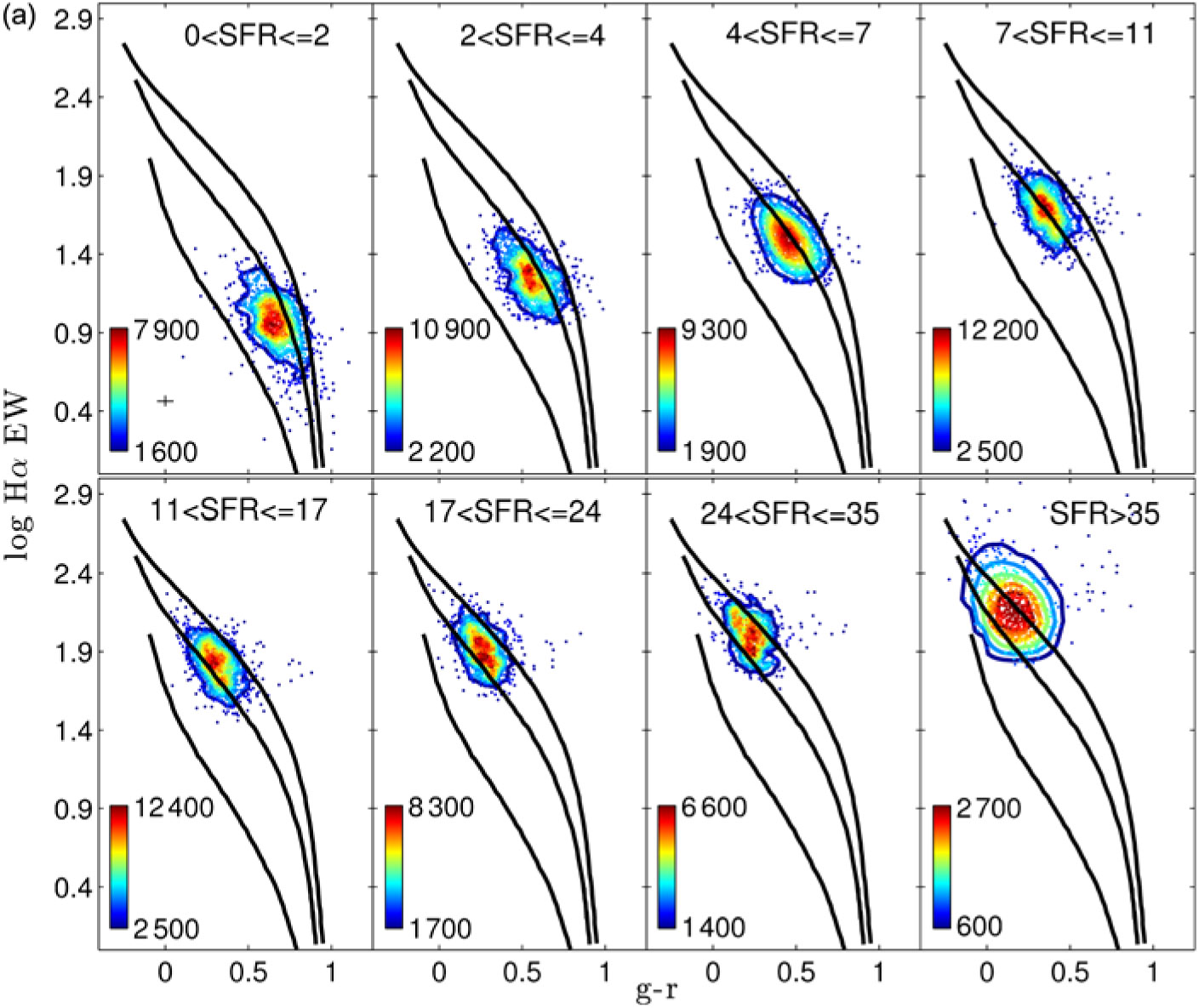
Figure 3. Following Kennicutt (Reference Kennicutt1983) and Hoversten & Glazebrook (Reference Hoversten and Glazebrook2008), this diagnostic shows how IMFs with different αh can be discriminated using the equivalent width of Hα and an optical colour, in this case (g – r). The solid tracks are the evolutionary paths followed through a star formation event, showing (top to bottom) the location expected for αh = –2, αh = –2.35, αh = –3. The data correspond to galaxies in the highest redshift bin of the three volume-limited samples, with ⟨z⟩ = 0.29, split into eight bins of SFR. This illustrates the tendency for the higher SFR systems to favour IMFs with flatter high-mass slopes (more positive αh). See Gunawardhana et al. (Reference Gunawardhana2011) for details. Reproduced from Figure 6a of ‘Galaxy and Mass Assembly (GAMA): the star formation rate (SFR) dependence of the stellar initial mass function’, Gunawardhana et al. (Reference Gunawardhana2011).
The same method was used by Gunawardhana et al. (Reference Gunawardhana2011) with data from the Galaxy and Mass Assembly survey (Driver et al. Reference Driver2011; Hopkins et al. Reference Hopkins2013; Liske et al. Reference Medling2015). Using three independent volume-limited galaxy samples spanning 0.1 ≲ z ≲ 0.35, they find a trend between the high-mass (m > 0.5 M⊙) IMF slope and SFR (Figure 3) or SFR surface density (ΣSFR). With the large sample available they are able to explore in detail the dependency of αh on these properties, which they quantify through the relations αh ≈ 0.36 log (SFR / M⊙ yr –1) – 2.6 or αh ≈ 0.3 log (ΣSFR / M⊙ yr –1 kpc –2) –1.7. For the range of SFR or ΣSFR they probed, this leads to a variation in the high-mass IMF slope from αh ≈ –2.5 for the least active star-forming systems (SFR ≈ 0.1 M⊙ yr –1) to αh ≈ –1.7 for the most active (SFR ≈ 50 M⊙ yr–1). They point out that for the current SFR of the Milky Way, these results would imply a value of αh ≈ –2.35, which is an encouraging consistency check. They also comment that the SFR dependence would imply a flatter high-mass IMF slope (αh > –2.35) in the Milky Way’s early history, given that it had an elevated SFR in the past.
Gunawardhana et al. (Reference Gunawardhana2011) note that while the SFR is an IMF-dependent quantity, applying an IMF-dependent SFR calibration would not qualitatively alter their conclusions, since the variation seen is monotonic, and would only have the effect of reducing the range of SFR sampled. Gunawardhana et al. (Reference Gunawardhana2011) also explore degeneracies in the variation of the IMF that would lead to the same observed combination of Hα equivalent width and g – r colour. They show that while the high-mass slope can be fixed at the Salpeter value (αh = –2.35) and the results explained by allowing mc to increase, it requires a very high value of mc ≈ 10 M⊙ to account for the highest star-forming systems, reminiscent of the early results for starburst nuclei (Rieke et al. Reference Rieke, Lebofsky, Thompson, Low and Tokunaga1980) that are no longer favoured (Elmegreen Reference Elmegreen, Kang, Lee, Leung and Cheng2007).
Again to rule out the possibility that stochastic SFHs could be the origin of the observed signature, Gunawardhana et al. (Reference Gunawardhana2011) extended the analysis of Hoversten & Glazebrook (Reference Hoversten and Glazebrook2008) by demonstrating that both stellar mass and mass-doubling time for the observed galaxies vary smoothly along the SPS model tracks. They found no signature corresponding to the significant bursts of star formation that would be seen if stochastic SFHs were the dominant effect. Subsequently, Nanayakkara et al. (Reference Nanayakkara2017), too, demonstrated quantitatively that stochastic star formation histories could not explain their measurements, in a sample at much higher redshift. Gunawardhana et al. (Reference Gunawardhana2011) further demonstrate that the result is robust to the implementation of dust correction and choice of population synthesis model. While there is a degeneracy between a varying high-mass αh and a varying mc, it is possible to exclude a variation in ml (Figure 4). It is clear that a varying low-mass cut-off has a very different signature in this diagnostic than a varying high-mass slope or mc. This confirms that the results of Gunawardhana et al. (Reference Gunawardhana2011) are not attributable to variations in ml while maintaining a Salpeter value for the high-mass slope.
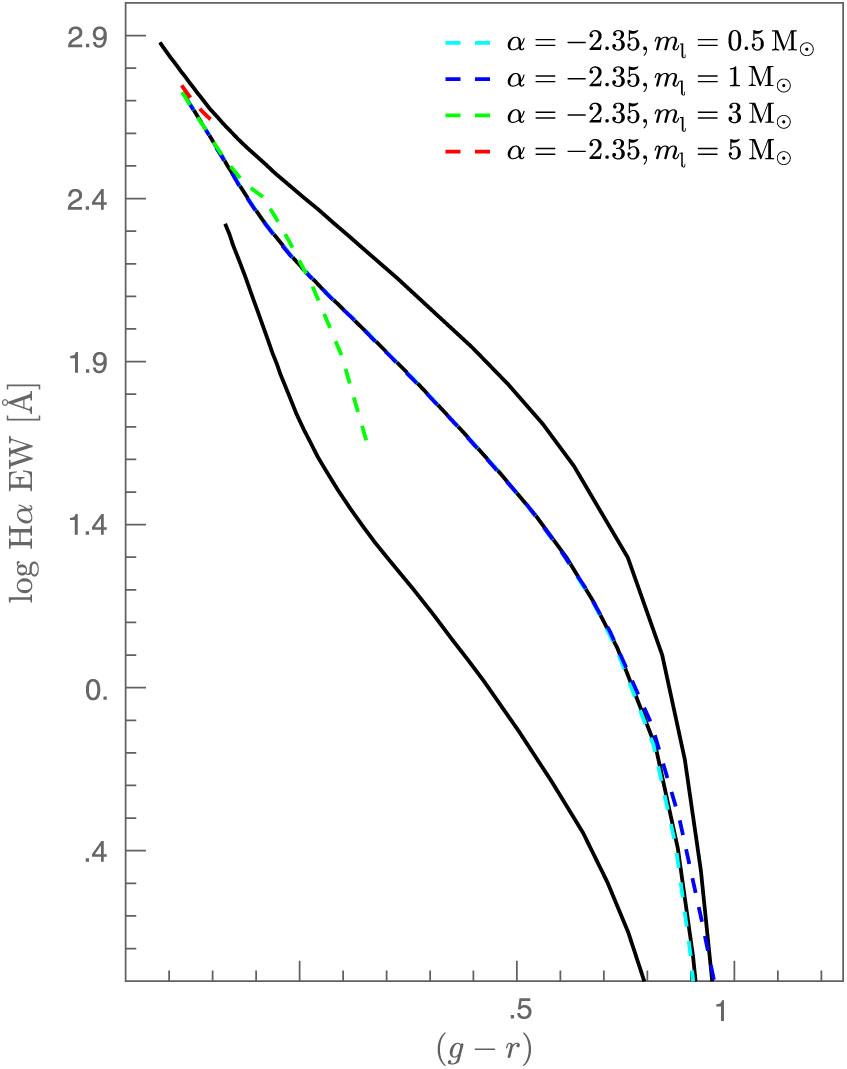
Figure 4. The IMF diagnostic used by Gunawardhana et al. (Reference Gunawardhana2011) to identify variations in the slope of the high-mass (m > 0.5 M⊙) IMF. The black solid lines show the evolutionary tracks expected for galaxies with, from top to bottom, αh = –2, –2.35, –3. The additional tracks (dashed coloured lines) illustrate the effect of a fixed high-mass slope (α = –2.35) but varying ml. The tracks become shorter as ml increases, due to the shorter lifetimes of the higher mass stars. Figure courtesy of M. Gunawardhana.
These results were extended to z ≈ 2 by Nanayakkara et al. (Reference Nanayakkara2017), finding that systems with the highest Hα equivalent widths could only be explained either by rotating extremely metal-poor stars with binary interactions, or IMFs with αh > –2 (0.5 < m / M⊙ <120). They note that in the latter case, no single IMF slope could reproduce the data, implying a need for a stochastically varying high-mass IMF slope. They explore the trend with SFR derived from Hα and from the combined UV and far-infrared (FIR) luminosities, finding a weak trend with the Hα SFR in the same sense as that of Gunawardhana et al. (Reference Gunawardhana2011), but none with the SFRs from the UV+FIR (Figure 21 of Nanayakkara et al. Reference Nanayakkara2017). This arises from the lowest Hα SFR systems having higher SFRs as measured by the UV+FIR. In order to avoid internal inconsistencies, it would be valuable for all analyses of this kind to present results in terms of IMF-independent quantities (such as luminosities) or to calculate SFRs or other IMF-dependent properties self-consistently assuming whatever IMF-dependency on αh or other parameter is being tested.
At similar redshifts, Zhang et al. (Reference Zhang, Romano, Ivison, Papadopoulos and Matteucci2018) measure the 13C/18O abundance ratio, probed through the rotational transitions of the 13CO and C18O isotopologues, for four starburst galaxies. These galaxies are gravitationally lensed submillimetre galaxies spanning 2.3 < z < 3.1. They find low ratios compared to chemical evolutionary models for the Milky Way, implying considerably more high-mass stars in such starbursts than in typical spiral galaxies, and with a high-mass slope flatter than that of Kroupa (Reference Kroupa2001).
At the opposite end of the scale, the Buat et al. (Reference Buat, Donas and Deharveng1987) approach relying on Hα-to-UV flux ratios has more recently been used to focus on potential variations to the IMF for low-mass or low SFR galaxies. The results of Meurer et al. (Reference Meurer2009), Lee et al. (Reference Lee2009), and Boselli et al. (Reference Boselli, Boissier, Cortese, Buat, Hughes and Gavazzi2009) all suggest that for low SFR (or low luminosity, or low mass) galaxies, there is evidence of a deficiency of high-mass stars, characterised as an IMF slope steeper than Salpeter (α < –2.35 for 0.1 < m/M⊙ < 100). As the Hα luminosity (or surface density) decreases within various samples of nearby galaxies, these authors show that the Hα luminosity (or flux) declines faster than that of the UV. This is in the opposite sense than could be explained through dust obscuration, which affects the UV proportionally more than Hα, although different levels of attenuation for the line and continuum emission may play some role (e.g. Charlot & Fall Reference Charlot and Fall2000). Pflamm-Altenburg, Weidner, & Kroupa (Reference Pflamm-Altenburg, Weidner and Kroupa2009) demonstrate how this result can arise within the IGIMF formalism.
After exploring and ruling out a range of possible scenarios, including dust obscuration, SFH, stochastic population of the IMF, metallicity, and escape fraction, Meurer et al. (Reference Meurer2009) conclude that the most likely scenario is a variation in the high-mass end of the IMF, with either mu ranging over 30 ≲ mu/M⊙ ≲ 120 or having a varying IMF slope spanning –3.3 ≲ α ≲ –1.3 (for 0.1 < m/M⊙ <100), in the sense that the lower SFR systems have either lower mu or steeper α. It is worth noting the use of the single power law IMF slope extending to the lowest masses here, and questioning whether a slope change below some mc would affect the results. Since the diagnostic uses flux ratios of indicators sensitive only to high-mass stars, though, it seems unlikely that changing this assumption would alter the IMF conclusions significantly.
The results of Meurer et al. (Reference Meurer2009) are qualitatively similar to those of Gunawardhana et al. (Reference Gunawardhana2011), with a high-mass IMF slope that gets progressively steeper as ΣSFR becomes lower. Quantitatively, though, the results are somewhat different, with Meurer et al. (Reference Meurer2009) inferring steeper IMF slopes at a given value of ΣSFR (or equivalently, ΣHα) than Gunawardhana et al. (Reference Gunawardhana2011), when retaining the same mu. Specifically, as an example, at log(ΣSFR/M⊙ yr –1 kpc –2) = –2.7 Gunawardhana et al. (Reference Gunawardhana2011) find αh ≈ –2.4 (Gunawardhana et al. Reference Gunawardhana2011, Figure 13c). This value of ΣSFR corresponds to log (ΣHα / Wkpc –2) = 31.4, for which Meurer et al. (Reference Meurer2009) find a typical value of log ((FHα/ fFUV) / Å) ≈ 0.65 (Meurer et al. Reference Meurer2009, Figure 3), and which leads to αh ≈ –3.0 (Meurer et al. Reference Meurer2009, Figure 10b). I return to exploring the details of these quantitative differences below.
Again in a qualitatively similar fashion, Boselli et al. (Reference Boselli, Boissier, Cortese, Buat, Hughes and Gavazzi2009) find that the IMF slope (for 0.1 < m/M⊙ <100) spans –2.6 ≲ α ≲ –2.3, with steeper slopes for the lower mass galaxies. Comparing quantitatively to Gunawardhana et al. (Reference Gunawardhana2011), these slopes are closer than inferred by Meurer et al. (Reference Meurer2009) but still rather steeper for a given stellar mass or sSFR. Based on Figure 10 of Boselli et al. (Reference Boselli, Boissier, Cortese, Buat, Hughes and Gavazzi2009), α = –2.5 is favoured for galaxies with 9.2 <log (M/M⊙), for example. This corresponds broadly to a range of –10 ≲ log(sSFR/yr –1) ≲ –9 (see Figure 4 of Bauer et al. Reference Bauer2013) for the GAMA sample in the redshift range analysed by Gunawardhana et al. (Reference Gunawardhana2011). For this range of sSFR, Gunawardhana et al. (Reference Gunawardhana2011) find high-mass IMF slopes spanning –2.4 ≲ αh ≲ –2.1 (Gunawardhana et al. Reference Gunawardhana2011, Figure 13b), somewhat flatter than the α = –2.5 of Boselli et al. (Reference Boselli, Boissier, Cortese, Buat, Hughes and Gavazzi2009).
Boselli et al. (Reference Boselli, Boissier, Cortese, Buat, Hughes and Gavazzi2009) invoke bursty SFHs to explain their findings in preference to IMF variations, contradicting the claim by Meurer et al. (Reference Meurer2009) that the ‘gasps’ between such bursts would have to be unrealistically synchronised between galaxies to produce the range of measured flux ratios. Boselli et al. (Reference Boselli, Boissier, Cortese, Buat, Hughes and Gavazzi2009) note that the star formation in dwarf galaxies can be dominated by a single H ii region, which can lead to larger scatter in the Hα to UV flux ratio than for high-mass galaxies, arising from the different lifetimes of the OB stars (∼106 yr) responsible for the Hα emission and the A stars (∼107 yr) responsible for the UV emission.
Lee et al. (Reference Lee2009) use a nearby sample of galaxies to probe to extremely low levels of SFR, down to SFR ≈ 10–4 M⊙ yr –1 and see very similar effects to the results of Meurer et al. (Reference Meurer2009) and Boselli et al. (Reference Boselli, Boissier, Cortese, Buat, Hughes and Gavazzi2009). They do not attempt to constrain the IMF directly but instead test (and rule out) a variety of explanations, while noting that the IGIMF predictions of Pflamm-Altenburg et al. (Reference Pflamm-Altenburg, Weidner and Kroupa2009) match their observations surprisingly well, before also implying a preference for SFH variations (bursty or ‘flickering’) as a possible explanation (see also Lee et al. Reference Lee, Gil de Paz, Tremonti, Kennicutt, Treyer, Wyder, Neill, Seibert and Lee2011). In contrast, Fumagalli, da Silva, & Krumholz (Reference Fumagalli, da Silva and Krumholz2011) argue, based on a stochastic code for synthetic photometry, that these observed Hα-to-UV flux ratios in low SFR galaxies can be explained by random sampling from a ‘universal’ IMF, combined with stellar evolution. A similar result was found by Weisz et al. (Reference Weisz2012) who note that such stochastic SFHs can explain the observed Hα to UV flux ratios in low-mass galaxies, without invoking IMF variations.
Bearing in mind the likely contributions of stochastic SFHs, there does seem to be some evidence for the idea that systems with lower luminosities, masses, or SFRs favour IMFs lacking in high-mass stars relative to a Kroupa (Reference Kroupa2001) or Chabrier (Reference Chabrier2003a) IMF. This is reinforced by studies of the LMC, SMC, and other dwarf, low metallicity, or low surface brightness galaxies. Using UV imaging of the LMC and models jointly constraining IMF slope, obscuration, and age, Parker et al. (Reference Parker1998) find αh = –2.80 ±0.09 (for m ≳ 7 M⊙). Lamb et al. (Reference Lamb, Oey, Graus, Adams and Segura-Cox2013) find αh = –3.3±0.4 (for m > 20 M⊙) in the SMC based on spectra for a spatially complete census of field OB stars. The dwarf starburst galaxy NGC 4214 was found by Úbeda, Maíz-Apellániz, & MacKenty (Reference Úbeda, Maíz-Apellániz and MacKenty2007) to have αh < –2.83±0.07 (for 20 < m/M⊙ <100), the upper limit arising due to the presence of unresolved binaries, the neglect of which acts to flatten the inferred IMF. Lee et al. (Reference Lee, Gibson, Flynn, Kawata and Beasley2004) use the high M/L ratios for seven low surface brightness disk galaxies to estimate α = –3.85 (for 0.1 < m/M⊙ < 60). Garcia et al. (Reference Garcia, Herrero, Najarro, Camacho, Lennon, Urbaneja, Castro, Eldridge, Bray, McClelland and Xiao2017) summarise studies of high-mass stars in Local Group dwarf galaxies with very low metallicity, oxygen abundances less than 1/7 of the solar value. Although relying on a sample of only four galaxies, with incomplete observations of the high-mass stellar population, they note that the highest mass stars so far identified have initial masses of m ≈ 60 M⊙. Bruzzese et al. (Reference Bruzzese, Meurer, Lagos, Elson, Werk, Blakeslee and Ford2015) explore the IMF of the dark-matter dominated, extremely low SFR, blue compact dwarf galaxy NGC 2915, and reinforce the possibility of high-mass IMF slopes rather steeper than Salpeter for such systems. They combine colour magnitude diagrams for the stellar populations with an assumed recent SFH to find a high-mass IMF slope αh = –2.85 (for m ≳ 4 M⊙) and a poorly constrained upper mass limit of mu = 60 M⊙. Noting the impact of assuming a constant recent SFH (Elmegreen & Scalo Reference Elmegreen and Scalo2006), the IMF may not be quite this extreme, although it is not inconsistent with the other results highlighted here, in similar environments. The same approach, assuming a constant SFR over the dynamical timescale, was used in inferring the IMF of the dwarf irregular galaxy DDO 154 by Watts et al. (Reference Watts, Meurer, Lagos, Bruzzese, Kroupa and Jerabkova2018), to derive αh = –2.45 with a similarly poorly constrained mu = 16 M⊙.
For the population of ultra-compact dwarf galaxies (UCDs), known to have high V-band mass-to-light ratios (ϒV), Dabringhausen, Kroupa, & Baumgardt (Reference Dabringhausen, Kroupa and Baumgardt2009) use population synthesis modelling to infer αh, after arguing that the non-baryonic dark matter contribution is too low to influence the dynamics of these systems (Murray Reference Murray2009). Contrary to the results above for other dwarf galaxy systems, they show that an IMF with a relative excess of high-mass stars, αh ≈ –1.6 to αh ≈ –1.0 (depending on the assumed age), is required to account for the observed ϒV. This perhaps highlights SFR density as a significant factor in shaping the IMF. In contrast to the local dwarf systems, which are typically low surface density galaxies, the UCDs are expected to have formed rapidly, with SFRs as high as perhaps 10–100 M⊙ yr –1, and a correspondingly high ΣSFR given their small physical sizes. For a physical scale of 10 pc this would give 5 ≲ log (ΣSFR/M⊙ yr –1kpc –2)≲6, substantially higher than in the population of higher mass galaxies discussed above. The elevated values of αh inferred are qualitatively consistent with the results for higher mass star-forming galaxies, although any potential dependence of αh on ΣSFR is quantitatively inconsistent with the nominal linear relations of Meurer et al. (Reference Meurer2009), Gunawardhana et al. (Reference Gunawardhana2011), or Nanayakkara et al. (Reference Nanayakkara2017).
Using UV spectral lines as a constraint, Leitherer (Reference Leitherer, Treyer, Wyder, Neill, Seibert and Lee2011) combines measurements for a sample of 28 nearby galaxies (distances less than 250 Mpc) to construct the average UV spectrum and concludes that the high-mass (m > 0.5 M⊙) IMF slope is constrained to lie between –2.6 ≲ αh ≲ –2.0. This range encompasses most of the variation in αh inferred from the studies described above, and consequently does not substantially rule out the proposed variations.
With the exception of the dwarf galaxies and low surface brightness galaxies, which show rather steeper high-mass (m > 0.5 M⊙) IMF slopes (although noting the opposite result for UCDs, which are perhaps more analogous to starburst systems), the range spanned by αh from these investigations is not large, with most galaxies having −2.5 ≲ αh ≲ − 1.8 (e.g. Gunawardhana et al. Reference Gunawardhana2011), similar to the range seen in nearby stellar populations and star clusters, and variously attributed to observational or astrophysical limitations. It is notable that Gunawardhana et al. (Reference Gunawardhana2011) place the Milky Way on their relationship between α and SFR or ΣSFR, finding a Salpeter IMF slope (αh = −2.35) consistent with the bulk of analyses of Galactic stellar populations.
In summary, the observations for star-forming galaxies suggest a broadly consistent picture in favour of IMF variations, with αh larger (flatter) for higher SFR or ΣSFR, and smaller (steeper) for lower SFR or ΣSFR. This is in line, qualitatively at least, with the results seen above for starburst or super star clusters.
5.3. Passive galaxies
The descriptor ‘passive’ is intended here to refer to the degree of star formation, or rather its absence at any significant level, and is independent of the existence or not of an AGN. The methods of Kennicutt (Reference Kennicutt1983) and Buat et al. (Reference Buat, Donas and Deharveng1987) are not typically able to be applied to passive galaxies, as they have little or no Hα and UV emission arising from high-mass young stars. Where such emission is present it is likely to arise from, and be dominated by, an AGN rather than star formation. Also, since the stars being probed in these passive galaxies are only those low-mass objects remaining from star formation episodes much earlier, any IMF measured in such systems is in a sense a ‘relic’ IMF, analogous to the PDMF in Milky Way stellar systems, and in many cases this has led naturally to a focus on the low-mass end of the IMF.
A novel approach was explored by van Dokkum (Reference van Dokkum2008), noting the opposing effect of the IMF on luminosity and colour evolution identified by Tinsley (Reference Tinsley1980), such that an IMF with proportionally more high-mass stars would lead to stronger luminosity evolution and weaker color evolution. He compared the rate of luminosity and colour evolution for high-mass elliptical galaxies in clusters spanning 0 ≤ z ≤ 0.83 and found a need for an IMF with  $ \alpha {\kern 1pt} = {\kern 1pt} - 0.7_{ - 0.4}^{ + 0.7} $ at masses around m ≈ 1 M⊙, much flatter than a Kroupa (Reference Kroupa2001) or Chabrier (Reference Chabrier2003a) IMF at these masses, to explain the observations. Casting this as an estimate of $ {m_c} = 1.9_{ - 1.2}^{ + 9.3}{\kern 1pt} {{\rm{M}}_ \odot } $ at $ z = 3.7_{ - 0.8}^{ + 2.3} $ (the estimated formation redshift of stars at this stellar mass) for a Chabrier-like IMF, and comparing with the lower inferred values of mc at lower redshift, he goes on to explore the impact of an evolving mc. He notes the effect of reducing the apparent discrepancy between the cosmic SFH and SMD, confirming similar results (Hopkins & Beacom Reference Hopkins and Beacom2006; Fardal et al. Reference Fardal, Katz, Weinberg and Davé2007; Wilkins et al. Reference Wilkins, Trentham and Hopkins2008a), and which I discuss in detail in Section 6. The result of van Dokkum (Reference van Dokkum2008) was questioned by van Dokkum & Conroy (Reference van Dokkum and Conroy2012) who show instead that when comparing galaxies at a given velocity dispersion, rather than stellar mass, the observed luminosity and colour evolution is consistent with the standard Salpeter slope.
More recent approaches have focused on using spectral signatures sensitive to the dwarf-to-giant ratio, stellar mass-to-light ratios, and kinematics to explore the inferred IMF.
The dwarf-to-giant ratio approach evolved from early work using Na i D lines as a tracer of dwarf star populations (Spinrad Reference Spinrad1962) which concluded that the most luminous and high-mass elliptical galaxies showed evidence for proportionally more dwarf stars than found in lower mass galaxies. Additional spectral features (Mg i, Ca i, Ca ii, TiO, CN, CH, CaH, MgH) sensitive to different stellar populations (Spinrad Reference Spinrad1966; Wood Reference Wood1966; Spinrad & Taylor Reference Spinrad and Taylor1971) enabled improvement of the ability to characterise the stellar populations present in integrated galaxy spectra. Whitford (Reference Whitford1977) incorporated measurements of the Wing–Ford molecular band at 9910 Å to argue against the earlier results that favoured an excess of dwarf stars in such galaxies, ruling out IMFs with α ≤ −3, and finding results supporting an IMF with α ≈ −2.
Figure 5. Three spectral regions showing features sensitive to the presence or absence of low-mass stars (upper panels), and the trend in the absorption strength of those features seen with velocity dispersion of the galaxies (lower panels). This demonstrates that galaxies with higher velocity dispersion, and hence higher stellar mass, have a tendency to favour an excess of dwarf, or low-mass, stars. See van Dokkum & Conroy (Reference van Dokkum and Conroy2012) for details. (Figure 10 of ‘The stellar initial mass function in early-type galaxies from absorption line spectroscopy. I. Data and empirical trends,’ van Dokkum & Conroy (Reference van Dokkum and Conroy2012), © AAS. Reproduced with permission.)
This general technique has been developed significantly through recent work (e.g. van Dokkum & Conroy Reference van Dokkum and Conroy2010, Reference van Dokkum and Conroy2012) and is illustrated by Figure 5, which has been reproduced from van Dokkum & Conroy (Reference van Dokkum and Conroy2012). A key result was that of van Dokkum & Conroy (Reference van Dokkum and Conroy2010), who apply the high resolution SPS models of Conroy, Gunn, & White (Reference Conroy, Gunn and White2009) to estimate the proportion of low-mass dwarf stars (m < 0.3 M⊙) necessary to explain the observed absorption in the Na iλλ 8183,8185 Å doublet and the Wing–Ford FeH band around λ 9916Å for eight nearby elliptical galaxies in the Virgo and Coma clusters. They infer αl ≈ −3 for the low-mass range (0.1 < m/M⊙ < 0.3), significantly steeper than the Salpeter slope. As these stars would have formed at high redshift (z = 2−5), they argue against high redshift IMFs with a deficit of low-mass stars such as the truncated IMF of Baugh et al. (Reference Baugh, Lacey, Frenk, Granato, Silva, Bressan, Benson and Cole2005). Recall that for the Milky Way −1.4 ≲ αl ≲ −0.6 from the compilation of Bastian et al. (Reference Bastian, Covey and Meyer2010). van Dokkum & Conroy (Reference van Dokkum and Conroy2012) and Conroy & van Dokkum (Reference Conroy and van Dokkum2012) extended this result to the bulge of M31 and 34 galaxies from the SAURON integral field spectroscopy sample (Bacon et al. Reference Bacon2001), adding the Ca ii λλ 8498,8542,8662 Å triplet to the diagnostics, and concluding that the low-mass m < 0.3 M⊙ IMF slope varies systematically with galaxy velocity dispersion and α-enhancement, with steeper slopes in more massive and high-abundance galaxies (Figure 5).
Using similar approaches, both Spiniello et al. (Reference Spiniello, Trager, Koopmans and Chen2012) and Ferreras et al. (Reference Ferreras, La Barbera, de la Rosa, Vazdekis, de Carvalho, Falcón-Barroso and Ricciardelli2013) infer IMF slopes for the same mass range steeper than Salpeter (αl ≈ −3) for high velocity dispersion systems (σ ≳ 300 km s–1), and La Barbera et al. (Reference La Barbera, Ferreras, Vazdekis, de la Rosa, de Carvalho, Trevisan, Falcón-Barroso and Ricciardelli2013) also find IMF slopes steeper than Salpeter for systems with σ ≳ 220 km s–1. Zaritsky, Gil de Paz, & Bouquin (Reference Zaritsky, Gil de Paz and Bouquin2014a) find a strong correlation between UV colour and ϒ* for the same sample of galaxies analysed by van Dokkum & Conroy (Reference van Dokkum and Conroy2012) and conclude that this correlation is attributable to varying populations of extreme horizontal branch stars arising from the IMF variations.
For lower stellar mass systems, Smith et al. (Reference Smith, Lucey and Carter2012) analysed 92 red-sequence galaxies in the Coma cluster, including more galaxies with lower velocity dispersions than van Dokkum & Conroy and (Reference van Dokkum and Conroy2012) and Conroy & van Dokkum (Reference Conroy and van Dokkum2012). They found no clear dependence of IMF slope on velocity dispersion with a Salpeter slope adequate for 100 ≲ σ/kms –1 ≲ 250 (although they do not rule out steeper IMF slopes at higher velocity dispersions), but they do see a dependence on α-enhancement (Mg/Fe ratio), concluding that the IMF variation arises as a result of star formation mode, with rapid bursts leading to proportionally more low-mass stars (m < 0.3 M⊙).
In parallel with these analyses, gravitational lensing and dynamical constraints were being explored as a tool for inferring mass-to-light ratios (ϒ) and placing associated constraints on IMF slopes. This approach was refined by Treu et al. (Reference Treu, Auger, Koopmans, Gavazzi, Marshall and Bolton2010) who infer ϒ for 56 galaxies from the SLACS survey (Bolton et al. Reference Bolton, Burles, Koopmans, Treu and Moustakas2006). They introduce an IMF mismatch parameter, also denoted α, which is defined to be the ratio of ϒ inferred independently from the lensing and dynamical analysis compared to that from SPS modelling. For clarity, I refer to the IMF mismatch parameter as αmm = ϒLD/ϒSPS throughout.
Treu et al. (Reference Treu, Auger, Koopmans, Gavazzi, Marshall and Bolton2010) find that, with the assumption of an NFW dark matter profile (Navarro, Frenk, & White Reference Navarro, Frenk and White1996), such galaxies tend to favour IMFs such as Salpeter that provide a higher ϒ* than those of Chabrier (Reference Chabrier2003a). While stellar mass range is not discussed, the Bruzual & Charlot (Reference Bruzual and Charlot2003) models used span a mass range of 0.1 ≤ m/M⊙ ≤ 100, and from the scale of the IMF mismatch parameter it is reasonable to infer that the Salpeter IMF slope (α = −2.35) is applied over that full range for their Salpeter SPS mass estimates (confirmed by T. Treu, personal communication). Treu et al. (Reference Treu, Auger, Koopmans, Gavazzi, Marshall and Bolton2010) also note that their sample is limited to relatively high velocity dispersion systems, and show that, while for galaxies with σ ≈ 200 km s–1 a Chabrier (Reference Chabrier2003a) IMF provides consistent ϒ* with the lensing and dynamical estimate, ‘heavier’ IMFs (i.e. with a greater total mass normalisation) are required for higher velocity dispersion systems. They conclude that either the IMF varies towards one with a Salpeter-like mass normalisation for the most massive galaxies, or that dark matter profiles are not universal and the inner slope is systematically steeper than NFW for the most massive galaxies, or possibly a combination of both. This result is still not as extreme as the αl ≈ −3 found spectroscopically by van Dokkum & Conroy (Reference van Dokkum and Conroy2010).
Similarly, Läsker et al. (Reference Läsker, van den Bosch, van de Ven, Ferreras, La Barbera, Vazdekis and Falcón-Barroso2013) use a combination of dynamical models and the SPS and IMF approach of Vazdekis et al. (Reference Vazdekis, Casuso, Peletier and Beckman1996, Reference Vazdekis, Ricciardelli, Cenarro, Rivero-González, Díaz-García and Falcón-Barroso2012) to infer an IMF with a steep high-mass slope, (αh = −4.2±0.1 for m > 0.6 M⊙ constraining αl = −1.3 for 0.1 < m/M⊙ < 0.6) in a low redshift (z = 0.116) high-mass (σ=360 km s–1) early-type galaxy with a putative extremely high-mass nuclear black hole. In apparent contrast to these results, though, Smith & Lucey (Reference Smith and Lucey2013) used gravitational lensing mass estimates to demonstrate that ϒ* for a high-mass (σ ≈ 330 km s–1) low-redshift (z = 0.035) giant elliptical is consistent with a Kroupa (Reference Kroupa2001) IMF. This result was subsequently reinforced by Smith, Lucey, & Conroy (Reference Smith, Lucey and Conroy2015a) who analysed three high-mass (σ > 300 km s–1) low redshift (z ≲ 0.05) galaxies, showing that the inferred IMF mass normalisation is consistent with that of Kroupa (Reference Kroupa2001), and excluding a Salpeter IMF (α = −2.35 over 0.1 < m/M⊙ < 100) at the 3.5 σ level.
These results, though, are not inconsistent with the scatter seen by Treu et al. (Reference Treu, Auger, Koopmans, Gavazzi, Marshall and Bolton2010) in their IMF mismatch parameter. It is worth reiterating that Treu et al. (Reference Treu, Auger, Koopmans, Gavazzi, Marshall and Bolton2010) use the observed small range of scatter on αmm to argue that ‘the absolute normalization of the IMF is uniform to better than 25%’, a result that echoes the relatively small range of potential variations found for the star-forming galaxy population, although with a different sense in the variation itself for the passive galaxies (i.e. higher mass passive galaxies favouring proportionally more low-mass stars, but higher mass star-forming galaxies favouring proportionally more high-mass stars).
There is a subtlety around gas recycling in SPS that affects the M/L ratio comparison technique. Whether the gas recycled through stellar evolution is retained or not in the SPS inferred masses has a direct impact on the comparison to masses inferred from lensing and dynamics. Treu et al. (Reference Treu, Auger, Koopmans, Gavazzi, Marshall and Bolton2010) explore the two extreme cases, where all gas lost through stellar evolution is removed, and where it is retained (the ‘zero age’ SPS mass). They note that for a Chabrier (Reference Chabrier2003a) IMF the ‘zero age’ masses tend to be overestimates compared to the lensing masses, implying that at least some fraction of the gas associated with recycling is expelled and does not contribute to the baryonic mass in the region probed by the lensing and dynamical constraints. In this and subsequent work, it is typically just the mass in stars and stellar remnants derived from the SPS that is compared with the lensing and dynamical mass estimates, which for early type galaxies with very low gas fractions is likely to be a reasonable assumption. It must be noted, though, that such mass estimates may be lower limits if some gas component still contributes non-negligibly to the baryonic mass and needs to be accounted for in the uncertainties on inferred IMF constraints.
Figure 6. The mass-to-light ratio for the stellar component of ATLAS3D galaxies estimated using dynamical models, (M/L)stars, compared to that estimated from spectral fitting using SPS models assuming a fixed Salpeter IMF, (M/L)Salp. This demonstrates the trend for the high mass-to-light, or high velocity dispersion, galaxies in this sample to favour IMFs with an excess of mass compared to the IMFs of Chabrier (Reference Chabrier2003a) or Kroupa (Reference Kroupa2001), approaching and exceeding that from a Salpeter slope over the full mass range (an excess of low-mass stars). See Cappellari et al. (Reference Cappellari2013) for details. Reproduced from Figure 11 of ‘The ATLAS3D project – XX. Mass-size and mass-σ distributions of early-type galaxies: bulge fraction drives kinematics, mass-to-light ratio, molecular gas fraction, and stellar initial mass function,’ Cappellari et al. (Reference Cappellari2013).
Another significant development around the same time was the use of stellar kinematics and dynamical models to constrain the IMF (Cappellari et al. Reference Cappellari2012, Reference Cappellari2013) illustrated in Figure 6. They used the ATLAS3D sample of 260 early-type galaxies (Cappellari et al. Reference Cappellari2011) combining the measured stellar kinematics with detailed axisymmetric dynamical models, to derive accurate stellar masses and mass-to-light ratios for the population. By comparing the mass-to-light ratio measured dynamically in this way to that inferred from the photometry using SPS models that assume a Salpeter IMF over the full mass range (0.1 < m/M⊙ < 100), they are able to show a systematic variation in the inferred IMF normalisation. This variation ranges from a mass normalisation consistent with Chabrier (Reference Chabrier2003a) or Kroupa (Reference Kroupa2001) at ϒ* ≈ 6 M⊙/L⊙ to one consistent with a Salpeter slope spanning 0.1 ≤ m/M⊙ ≤ 100 at ϒ* ≈ 6 M⊙/L⊙ (Figure 6). This may extend to even higher mass normalisations at the most extreme measured values of ϒ* ≈ 10 M⊙/L⊙, with an IMF characterised equally by α = −2.8 (dominated by low-mass stars) or α = −1.5 (dominated by high-mass stars). This result has been questioned by Clauwens, Schaye, & Franx (Reference Clauwens, Schaye and Franx2015), though, who note that these trends could also be produced if the kinematic mass estimates had Gaussian errors of the order of 30%.
There are significant degeneracies possible in IMF shape when only the mass normalisation is constrained. While this is highlighted for the very high-mass normalisations by Cappellari et al. (Reference Cappellari2013), that of a Salpeter IMF slope (α = −2.35) over the full mass range can also be reproduced by an IMF with a Milky Way style low-mass slope, and an excess of high-mass stars. By way of illustration, this is achieved (including only the mass in stars and stellar remnants) by an IMF with αl = −1.5 (0.1 ≤ m/M⊙ ≤ 0.5) and αh=−1.70 (0.5 ≤ m/M⊙ ≤ 100), or an IMF with the Kroupa (Reference Kroupa2001) low-mass slope αl = −1.3 (0.1 ≤ m/M⊙ ≤ 0.5) and αh = −1.64 (0.5 ≤ m/M⊙ ≤ 100). Different combinations can equally be used to match the zero-age mass normalisation. The point is that a value of ϒ* consistent with a Salpeter IMF over the full mass range does not necessarily imply an excess of low-mass stars. To break this degeneracy, Conroy et al. (Reference Conroy, Dutton, Graves, Mendel and van Dokkum2013) quantitatively compared the scale of the IMF mass normalisation derived using the dwarf-to-giant approach with that from dynamical mass constraints and found that they are consistent, inferring that the explanation lies in an excess of low-mass stars (m ≲ 1 M⊙).
There have also been a range of enhancements and refinements that combine lensing, dynamical, and SPS constraints. These results largely confirm the need for a low-mass IMF slope similar to the Salpeter value for high-mass early-type galaxies. Spiniello et al. (Reference Spiniello, Barnabè, Koopmans and Trager2015a), for example, find a low-mass slope of αl = −2.37 ± 0.12 and 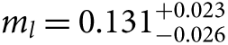 $ {m_l} = 0.131_{ - 0.026}^{ + 0.023}{\kern 1pt} {{\rm{M}}_ \odot } $ at a reference point corresponding to σ = 250 km s–1 for nine early-type galaxies, confirming earlier results by Barnabè et al. (Reference Barnabè, Spiniello, Koopmans, Trager, Czoske and Treu2013). In apparent contrast Lyubenova et al. (Reference Lyubenova2016), using 27 early-type galaxies from CALIFA (Walcher et al. Reference Walcher2014) and the IMF parameterisation approach of Vazdekis et al. (Reference Vazdekis, Casuso, Peletier and Beckman1996), rule out a single power law IMF and conclude that a double power law with a varying high-mass slope is required to explain the dynamical and stellar M/L ratios. This result may not be inconsistent with most of the results above, to the degree that it is only the mass normalisation that is being constrained through this approach, but it would be inconsistent with the conclusions of Conroy et al. (Reference Conroy, Dutton, Graves, Mendel and van Dokkum2013). Testing the consistency of IMF measurements between the SPS and the lensing and dynamical approaches is clearly important, and some work in this area has already begun (Newman et al. Reference Newman, Smith, Conroy, Villaume and van Dokkum2017). Using three strongly lensed passive galaxies, Newman et al. (Reference Newman, Smith, Conroy, Villaume and van Dokkum2017) find consistent IMF estimates between the two techniques for one galaxy, but require a variable low-mass cut-off or a non-parametric form of the IMF to reconcile the approaches for the remaining two systems. Clearly, extending such analyses to larger samples is desirable.
More recently these approaches have been extended to identify radial gradients in the IMF shape (van Dokkum et al. Reference van Dokkum, Conroy, Villaume, Brodie and Romanowsky2017). They characterise their results using a variant of the αmm IMF mismatch parameter which, instead of comparing dynamical to SPS M/L ratios, compares the ϒ* inferred from a given SPS fit to a canonical Milky Way IMF such as Kroupa (Reference Kroupa2001) or Chabrier (Reference Chabrier2003a) as a convenient shorthand for encapsulating the relative mass normalisation. Using αmm = ϒSPS/ϒMW in this way, they find IMFs with mass normalisations heavier than Kroupa (Reference Kroupa2001) or Chabrier (Reference Chabrier2003a) (αmm ≈ 2.5) in the central regions for six early-type galaxies, but approaching the Milky Way value as radius increases, with αmm ≈ 1.1 at R > 0.4 Re. The SPS IMF constraint approach has also been refined by Conroy, van Dokkum, & Villaume (Reference Conroy, van Dokkum and Villaume2017), who developed a non-parametric approach to constraining the m < 1 M⊙ shape. Applying this to the centre of NGC 1407, they find an IMF slope consistent with αl=−2.7. Such radial trends may provide an explanation for the differences found in the IMF properties between the spectroscopic and the dynamical approaches. It is also a tantalising link to the postulated ‘two-phase’ formation scenario for early type galaxies (e.g. González Delgado et al. Reference González Delgado2017), which proposes that the cores of elliptical galaxies formed quickly and quenched rapidly (the high redshift ‘red nuggets’), in contrast to their outer regions. Martín-Navarro et al. (Reference Martín-Navarro, La Barbera, Vazdekis, Ferré-Mateu, Trujillo and Beasley2015b) find a ‘bottom-heavy’ IMF (1.5 ≲ αmm ≲ 2) out to 1.5 Re in NGC 1277 and argue that this is an example of the kind of ‘core’ that would evolve through dry merging to the characteristic masses and sizes of z ≈ 0 elliptical systems.
Martín-Navarro et al. (Reference Martín-Navarro2015d) argue that metallicity, rather than velocity dispersion, is the driver of IMF variations in early type galaxies, building on their earlier work ((Martín-Navarro et al. Reference Martín-Navarro, La Barbera, Vazdekis, Falcón-Barroso and Ferreras2015a, Reference Martín-Navarro, La Barbera, Vazdekis, Ferré-Mateu, Trujillo and Beasley2015b) using the SPS and IMF parameterisation approach of Vazdekis et al. (Reference Vazdekis, Casuso, Peletier and Beckman1996). Using five key spectral features sensitive to metallicity, age, and the IMF, they add a sample of 24 galaxies from CALIFA to the earlier work, jointly constraining the metallicity and high-mass (m > 0.6 M⊙) IMF slope, with the low-mass (m < 0.6 M⊙) slope fixed at the Kroupa (Reference Kroupa2001) value (αl = –1.3). They find a metallicity dependence on the high-mass slope expressed as αh = −3.2(±0.1) −3.1(±0.5)[M/H], consistent with a Kroupa (Reference Kroupa2001) high-mass slope (αh = −2.3) for metallicities [M/H] ≈ −0.3, and steeper for higher metallicity. They also fit for a single power law, finding that the data could also be explained by an IMF with slope α = −2.5(±0.05)−2.1(±0.2)[M/H] over the full mass range (0.1 ≤ m/M⊙ ≤ 100). They go on to demonstrate that the relationship observed by other authors between IMF slope and stellar velocity dispersion naturally arises, qualitatively at least, through a combination of the mass–metallicity relation (e.g. Tremonti et al. Reference Tremonti2004; Lara-López et al. Reference Lara-López2013) and their derived IMF slope relation with metallicity. Martín-Navarro et al. (Reference Martín-Navarro2015d) further assert that the evolution in metallicity during galaxy formation implies an evolving IMF, drawing on arguments for IMFs dominated by high-mass stars in low metallicity environments (Marks et al. Reference Marks, Kroupa, Dabringhausen and Pawlowski2012) transitioning to IMFs with a relative excess of low-mass stars as the metallicity rapidly increases. They also point to similar arguments by Arrigoni et al. (Reference Arrigoni, Trager, Somerville and Gibson2010) in favour of an evolving IMF for early-type galaxies, based on chemical evolution in semi-analytic models. This conclusion contrasts with the analysis of 212 ATLAS3D early-type galaxies by McDermid et al. (Reference McDermid2014) who conclude that there are no strong trends between any of the stellar population-derived parameters (age, metallicity, [α/Fe]) and the IMF mass normalisation.
More significantly, perhaps, Martín-Navarro (Reference Martín-Navarro2016) show that, in order for passive galaxies to have both enhanced [Mg/Fe] ratios and an IMF overabundant in low-mass stars relative to the Salpeter slope (αl < −2.35), they must have had extremely short star formation episodes that imply exceptionally high SFRs at high redshift, SFR ≈ 105 M⊙ yr–1, which have not been observed. They present two possible scenarios to resolve this issue. The first invokes an IMF overabundant in both low and high-mass stars. The second argues for a time varying IMF, initially overabundant in high-mass stars to account for the chemical signature, evolving to one overabundant in low-mass stars at later times.
The results described above have generally used relatively low redshift galaxy samples. Exploring the higher redshift Universe (0.9 < z < 1.5) Martín-Navarro et al. (Reference Martín-Navarro2015c) use the TiO2 IMF-sensitive spectral feature and the Vazdekis et al. (Reference Vazdekis, Casuso, Peletier and Beckman1996) SPS and IMF parameterisation, finding αh = −4.2±0.2 (for m > 0.6 M⊙) for the most massive galaxies (with stellar masses M * > 1011 M⊙), and slightly less steep (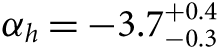 $ {\alpha _h} = - 3.7_{ - 0.3}^{ + 0.4} $) at lower stellar mass (2×10¹⁰ < M */M⊙ < 1011). With estimated ages of 1.7±0.3 Gyr, this population would have formed at redshifts of 1.5 ≲ z ≲ 3. These IMF slopes are similar to those found in the low redshift population for the highest metallicity galaxies by Martín-Navarro et al. (Reference Martín-Navarro2015d), which have similar formation epochs (z ≈ 2) based on the ages inferred in that analysis.
Using a different approach again, Dabringhausen et al. (Reference Dabringhausen, Kroupa, Pflamm-Altenburg and Mieske2012) measure the low-mass X-ray binary (LMXB) population in globular clusters and UCDs within 11 elliptical galaxies of the Virgo Cluster. They conclude that these are 10 times more frequent in UCDs than expected from a Kroupa (Reference Kroupa2001) IMF, implying an excess of high-mass stars. When the LMXB number is compared against an optical or infrared galaxy luminosity, this provides a direct constraint of the high-mass end of the IMF (the progenitors of the neutron stars and black holes detected as LMXBs) compared to the low-mass stellar population. In contrast, Peacock et al. (Reference Peacock, Zepf, Maccarone, Kundu, Gonzalez, Lehmer and Maraston2014) find no evidence for IMF variations in a sample of eight early-type galaxies, based on their LMXB population. Their results are based on a small sample, and are consistent with the range of scatter seen by Treu et al. (Reference Treu, Auger, Koopmans, Gavazzi, Marshall and Bolton2010). In either case, this demonstrates an important complementary approach to constraining the IMF. The presence of a low-mass companion in an LMXB also implies a degree of binarity that is often neglected in common SPS models. There is clearly scope to expand this kind of analysis to larger samples and through incorporating such SPS models (e.g. Eldridge Reference Eldridge2012; Eldridge et al. Reference Eldridge, Stanway, Xiao, McClelland, Taylor, Ng, Greis and Bray2017).
Other complementary approaches that have been recently explored for estimating integrated galaxy IMFs include the demonstration by Recchi et al. (Reference Recchi, Calura, Gibson and Kroupa2014) of how the plateau in the [α/Fe] ratio for a galaxy is sensitive to the galaxy IMF and can be used as a test of whether IMFs vary between galaxies. Brewer et al. (Reference Brewer, Marshall, Auger, Treu, Dutton and Barnabè2014) present a hierarchical modelling approach that can be used to derive upper limits on departures from universality in the IMF. Podorvanyuk et al. (Reference Podorvanyuk, Chilingarian and Katkov2013) introduce a pixel-based SPS fitting approach, similar to the ‘pixel-z’ technique (Conti et al. Reference Conti2003; Welikala et al. Reference Welikala, Connolly, Hopkins, Scranton and Conti2008, Reference Welikala, Connolly, Hopkins and Scranton2009) that fits pixel colours to infer stellar population ages, obscurations and SFHs. The approach of Podorvanyuk et al. (Reference Podorvanyuk, Chilingarian and Katkov2013) allows the IMF slope at the low-mass end to be a free parameter in the library of models generated and fit to the observed pixel colours, in principle allowing the IMF to be inferred within spatially resolved galaxy images. Geha et al. (Reference Geha2013) use resolved star counts of two nearby ultra-faint dwarf galaxies to determine  $ {\alpha _l} = - 1.2_{ - 0.4}^{ + 0.5} $ (Hercules) and αl = −1.3±0.8 (Leo IV) in the mass range 0.52 ≤ m/M⊙ ≤ 0.77, and argue that, in combination with resolved star counts from the Milky Way, SMC, and Ursa Minor, this suggests a trend to flatter low-mass IMF slopes (or increasing mc) for systems with lower velocity dispersion and metallicity, qualitatively consistent with the broad results seen for early type galaxies summarised above (e.g. van Dokkum & Conroy Reference van Dokkum and Conroy2012).
As with the star-forming galaxies, the range of analyses of passive galaxies reveal a broadly consistent picture, finding an increased abundance of low-mass stars for higher velocity dispersion, or higher metallicity, galaxies, and potentially with this excess located preferentially in the galaxy cores. These IMF variations for passive galaxies do seem to contradict the sense of the variation found for star-forming galaxies, a point that I return to below. It would also be interesting to explore the extent to which the recent generation of integral field spectroscopic surveys may be able to bridge the two, applying techniques so far used only for star-forming galaxies but instead looking at passive systems with some residual star formation. With spatially resolved spectra, any AGN contributions may be identified and excluded to isolate star formation signatures in otherwise passive galaxies (e.g. Hampton et al. Reference Hampton2017; Medling et al. Reference Medling2018), allowing the Kennicutt (Reference Kennicutt1983), allowing the Kennicutt (Reference Kennicutt1983) and related approaches to be applied.
5.4. Summary and limitations
It is clear that analyses of the star-forming and passive galaxy populations have a rather different focus in terms of the IMF, of necessity, due to the available observational metrics. Work on the star-forming galaxy population has focused on the high-mass end of the IMF, and its potential dependence on luminosity, SFR, or SFR (surface) density, loosely characterised as star formation intensity. Analysis of the passive galaxy population, instead, has focused on the low-mass end of the IMF. The stars being probed in these systems are only the low-mass stars remaining from star formation episodes many Gyr earlier, analogous to the PDMF in Milky Way stellar systems. In qualitative terms the results can be summarised as:
There is evidence for αh (m ≲ 1 M⊙) variation in star-forming galaxies, with flatter (more positive) values in stronger star-forming galaxies (increasing SFR, sSFR, or luminosity), and vice-versa.
There is evidence for αl (m ≲ 1 M⊙) variation in passive galaxies, (or equivalently, steeper αh when αl = −1.3 for m < 0.6 M⊙ is constrained) with steeper (more negative) values in (at least the centres of) more high-mass passive galaxies (higher σ or metallicity).
There is a range of uncertainty, quantitative difference, and scatter around these general conclusions, but the broad picture seems to be well established given the observational approaches used.
This broad picture leads to an apparent tension, though, because at first glance the two qualitative results seem inconsistent. The stellar population in the centres of passive galaxies, that formed at the peak of cosmic star formation (z ≈ 2, e.g. Hopkins Reference Hopkins2004; Hopkins & Beacom Reference Hopkins and Beacom2006), have a relative excess of low-mass stars (that may be characterised broadly as α < –2.35), while the star-forming galaxies seem to imply that high star formation is associated with a relative excess of high-mass stars (similarly characterised broadly by α > −2.35). Are these results actually inconsistent or not? If the IMF is not universal, they are not necessarily inconsistent, as it may be the case that different physical conditions prevailed in the progenitors of high-mass elliptical galaxy nuclei, than seen now in high SFR galaxies at low redshift. The question needs to be answered by exploring the physical properties dominating the origin of a particular stellar mass distribution, and the physical conditions prevailing in the different systems at the time of star formation. This is reviewed in Section 7.
Before delving into those issues, it is worth questioning the robustness of the various observational approaches, and assessing the degree to which they may be systematically biased.
In each case, SPS models play a crucial role in the way an IMF slope is inferred. There are some fundamental limitations in even the most sophisticated modern SPS models, each of which focuses on one particular area of strength but without necessarily incorporating other facets, or coarsely modelling them in the interests of computational efficiency. Two main limitations are the neglect of stellar rotation (e.g. Brott et al. Reference Brott2011a, Reference Brott2011b; Levesque et al. Reference Levesque, Leitherer, Ekstrom, Meynet and Schaerer2012; Leitherer et al. Reference Leitherer, Ekström, Meynet, Schaerer, Agienko and Levesque2014) and stellar multiplicity (e.g. Eldridge Reference Eldridge2012; Eldridge et al. Reference Eldridge, Stanway, Xiao, McClelland, Taylor, Ng, Greis and Bray2017). These effects are not negligible, with perhaps up to 30% of high-mass main sequence stars produced through binary interaction (Sana et al. Reference Sana2012; de Mink et al. Reference de Mink, Sana, Langer, Izzard and Schneider2014). Binarity and stellar rotation may reinforce each other in some observable properties, as the modelling of binaries can provide effects similar to the inclusion of stellar rotation for single stars (Leitherer Reference Leitherer, Treyer, Wyder, Neill, Seibert and Lee2011). In particular, extreme rotation can lead to an increase in the Hα equivalent width by up to an order of magnitude compared to the assumption of no rotation, for the same SFH, in a window between 106.5 < t/yr < 107 (Leitherer et al. Reference Leitherer, Ekström, Meynet, Schaerer, Agienko and Levesque2014). This may lead to a need to reduce inferred SFRs (for example) in some analyses, and may well have an impact on inferred IMFs. Binaries add an extra dimension too, as binary mergers and mass transfer can lead to the presence of stars of higher mass than those in the initial population (Eldridge Reference Eldridge2012; Banerjee, Kroupa, & Oh Reference Banerjee, Kroupa and Oh2012). For example, using a binary population synthesis approach Suda et al. (Reference Suda2013) make the case for the Milky Way having an IMF dominated by high-mass stars at early times, subsequently evolving to the presently observed IMF, based on observations of CEMP stars. They note that in chemical evolution models the current Milky Way IMF would overpredict Type 1.5 SNe. While observational constraints on the degree of rotation and binarity (or multiplicity) fraction are challenging, it is clear that it is necessary to address these effects in refining any estimated IMFs.
It is also worth noting that the SPS models used to analyse star-forming galaxies are typically different from those used to analyse passive galaxies, again for the obvious reason that different codes focus on producing different diagnostics. It would be highly desirable to be able to cross-compare results between the two galaxy populations using a common SPS tool to eliminate any possibility that inconsistent conclusions regarding the IMF are related to SPS model systematics.
SPS models commonly used in the analysis of star-forming galaxies include PEGASE (Fioc & Rocca-Volmerange Reference Fioc and Rocca-Volmerange1997), STARBURST99 (Leitherer et al. Reference Leitherer1999), and GALAXEV, (Bruzual & Charlot Reference Bruzual and Charlot2003), as well as those incorporating a greater contribution from TP-AGB stars (Maraston Reference Maraston2005). The conclusions regarding IMF properties in star-forming galaxies are generally consistent between these different models, and authors often check that their results are not strongly dependent on the SPS model used (e.g. Meurer et al. Reference Meurer2009; Gunawardhana et al. Reference Gunawardhana2011). Nanayakkara et al. (Reference Nanayakkara2017) compared various diagnostics between the PEGASE, STARBURST99, and BPASS (Stanway, Eldridge, & Becker Reference Stanway, Eldridge and Becker2016) SPS tools, to confirm that their results were not sensitive to the choice of SPS model.
In the analysis of passive galaxies, the two dominant SPS tools are the FSPS code of Conroy et al. (Reference Conroy, Gunn and White2009) and its recent variants (Conroy et al. Reference Conroy, van Dokkum and Villaume2017), and that of Vazdekis (Reference Vazdekis1999) and its recent variants (Vazdekis et al. Reference Vazdekis, Sánchez-Blázquez, Falcón-Barroso, Cenarro, Beasley, Cardiel, Gorgas and Peletier2010, Reference Vazdekis, Ricciardelli, Cenarro, Rivero-González, Díaz-García and Falcón-Barroso2012) based on the MILES/MIUSCAT empirical stellar spectral libraries. The higher resolution of these libraries is important for constraining the key absorption features sensitive to the low-mass stellar populations. Analyses using the former tend to be cast in terms of single power law IMF slopes, while those of the latter explore both single and double power law forms. Broadly, both approaches tend to conclude that high-mass (or high metallicity) early-type galaxies have a need for IMFs with a relative excess of low-mass stars, although this is achieved with different IMF forms depending on the SPS tool used for the analysis. Either a single power law IMF with a slope steeper than Salpeter (α < −2.35) or a double power law with a steep high-mass (m > 0.6 M⊙) slope, both leading to an excess of stars for m < 1 M⊙ compared to Milky Way type IMFs of Kroupa (Reference Kroupa2001) or Chabrier (Reference Chabrier2003b). Spiniello, Trager, & Koopmans (Reference Spiniello, Trager and Koopmans2015b) compare these two SPS models explicitly, and conclude that, while quantitatively different, the result implying an excess of low-mass stars for early type galaxies is qualitatively consistent between the two. Conroy (Reference Conroy2013) reviews SPS techniques and discusses what can reliably be measured. In this comprehensive review, issues of assumed metallicity and abundances, dust obscuration, SFHs, and stellar evolution libraries are addressed. In particular, Conroy (Reference Conroy2013) describes the impact on inferred IMFs arising from limitations in SPS models in his Section 7. He focuses primarily on the results arising from the passive galaxy analyses, concluding that modest IMF variations are supported, as inferred through ϒ* variations of a factor of 2–3. He briefly argues that the case for ‘top-heavy’ IMFs is not compelling, and does not explore the impact of SPS assumptions in those analyses.
Other potential issues affecting the use of the dwarf-to-giant ratio sensitive features are rare stellar populations and parameter degeneracies. Maccarone (Reference Maccarone2014) argue, for example, that barium stars and extrinsic S stars can explain the effects seen in the Wing–Ford band and the Na i D absorption features, without needing to invoke varying IMFs. Tang & Worthey (Reference Tang and Worthey2015) highlight strong degeneracies between the inferred IMF slope and the value of ml, the extent of AGB populations and variations in elemental abundances. They note that ‘increasing evidence shows that single-burst, single-composition stellar populations oversimplify the underlying stellar systems’ and conclude that it is very difficult to disentangle a steepening of the IMF slope from a decreased contribution of the AGB population in young metal-rich galaxies. They note that this degeneracy can be addressed using sufficiently high precision photometry and spectroscopy for old (10 Gyr) metal-rich populations. Similarly, Smith et al. (Reference Smith, Alton, Lucey, Conroy and Carter2015b) used composite J-band spectra compiled from over 100 galaxies to show that it is not possible to jointly constrain the Na abundance and the IMF slope in the most massive galaxies. They conclude by cautioning against over-reliance on Na lines in such studies.
Another limitation was highlighted by Smith (Reference Smith2014), who analysed the dynamical and SPS IMF constraints for 34 galaxies in common between those used by Conroy & van Dokkum (Reference Conroy and van Dokkum2012) and Cappellari et al. (Reference Cappellari2013). He found that while the general results of each are consistent, there is no correlation of the IMF inferred on a galaxy-by-galaxy level between the two approaches. He argues that the results of Conroy & van Dokkum (Reference Conroy and van Dokkum2012) are explained by a trend with Mg/Fe rather than σ, (perhaps qualitatively in line 2411 with Martín-Navarro et al. Reference Martín-Navarro2015d), but that Cappellari et al. (Reference Cappellari2013) finds no such relation. He concludes that a range of confounding factors (dark matter contributions or abundance patterns) have not been disentangled from the IMF effects in one or both of the methods. Interestingly, Oldham & Auger (Reference Oldham and Auger2016) show for M87 that introducing radial stellar anisotropy has a strong impact on the derived M/L, and that this leads to an inferred IMF consistent with Chabrier (Reference Chabrier2003a), although neglecting the anisotropy would lead to a value of ϒ* that implies a Salpeter-like IMF over 0.1 < m/M⊙ < 100.
It is also the case that many samples analysed to date are, in most cases, limited in number to a few tens or in some cases hundreds of galaxies. Although observationally challenging, there is clearly scope for exploring large volume-limited or mass-limited samples, as done by Gunawardhana et al. (Reference Gunawardhana2011), for example, in order to account for systematics and selection effects when interpreting any putative physical dependencies for potential IMF variations.
5.5. Linking galaxies to their constituents
The link between the IMF for stars or star clusters and that inferred for galaxies has been explored extensively in the framework of the IGIMF (Kroupa & Weidner Reference Kroupa and Weidner2003; Weidner & Kroupa Reference Weidner and Kroupa2005; Kroupa et al. Reference Kroupa, Weidner, Pflamm-Altenburg, Thies, Dabringhausen, Marks and Maschberger2013). Bastian et al. (Reference Bastian, Covey and Meyer2010) nicely summarise the link between the IGIMF and the relation between mu and cluster mass (Weidner et al. Reference Weidner, Kroupa and Bonnell2010), noting that the evidence for this relation is mixed (but see, e.g. Ramírez Alegría et al. Reference Ramírez Alegría2016; Stephens et al. Reference Stephens2017). It is worth a brief diversion here to consider a direct comparison between potential variations in the IMF for star clusters and that for galaxies, to test whether there are physical dependencies that may be consistent. From the summary of Bastian et al. (Reference Bastian, Covey and Meyer2010), Figure 2 of the reference has a suggestion that star clusters tend to have a somewhat flatter high-mass IMF slope (m > 1 M⊙) than found in associations or the field. Can this be characterised as a function of SFR or velocity dispersion, perhaps, to compare against the results from integrated galaxy measurements?
It is not straightforward, it turns out, to compare star-forming clusters directly with galaxies. The young massive star-forming cluster Westerlund 1 in the Milky Way, for example, has αh = −2.3 for stars in the mass range 3.4 < m/M⊙ < 27 (Brandner et al. Reference Brandner, Beuther, Linz and Henning2008). To compare this with the star-forming galaxies of Gunawardhana et al. (Reference Gunawardhana2011), say, we need to estimate one or more of its SFR, sSFR, or SFR surface density (Σ*). Brandner et al. (Reference Brandner, Beuther, Linz and Henning2008) quote a total initial stellar mass for Westerlund 1 of m ≈ 52 000 M⊙, an age of t ≈ 3.6 Myr, and they measured the IMF in annuli extending out to r = 3.3 pc. We can make use of these estimates by way of illustration, although the similarity of values for the other starburst clusters in the Milky Way (Brandner Reference Brandner, Beuther, Linz and Henning2008) lead to the same conclusions. Using the values above, SFR = 0.014 M⊙ yr–1, and Σ* ≈ 400 M⊙ yr–1 kpc–2 for Westerlund 1. It is apparent that the sSFR (defined as the SFR divided by the total stellar mass, for a galaxy) is not really a meaningful quantity here, since the total stellar mass is the same as the stellar mass formed in the star formation event and would simply equal the inverse of the age for the cluster. This is a hint that such comparisons are not easily made, quickly supported by the fact that the SFR surface density is two orders of magnitude higher than seen in the ensemble of galaxies sampled by Gunawardhana et al. (Reference Gunawardhana2011), where −2.7 ≲ log(Σ*/M⊙ yr −1 kpc −2)≲−0.8. Clearly the average Σ* for a galaxy is reduced by the many regions that have no ongoing star formation. Alternatively, we could artificially define a larger area encompassing Westerlund 1 that extends out to the boundary with the closest neighbouring star-forming system in order to define the value of Σ*, but that opens a host of related questions for how to define such a region. That leaves the direct measure of SFR itself. Here again the comparisons are not straightforward, since now the quantity for Westerlund 1 is two orders of magnitude lower than the range of SFR seen in the galaxies (0 ≲ log(SFR/M⊙yr –1)≲1.7), unsurprisingly when comparing a single star cluster to a whole galaxy. If instead the stellar velocity dispersion is used as the linking factor, star clusters again have σ substantially lower than those of galaxies. The super star clusters in M82, for example, have 10 ≲ σ/km s −1 ≲ 35 (McCrady & Graham Reference McCrady and Graham2007), compared to the range of 100 ≲ σ/km s −1 ≲ 350 for the early type galaxies in the analyses described above. Said another way, approaches that parameterise the IMF as a function of SFR or σ only make sense in the case of an entire galaxy where such parameters themselves are well-defined. Any relation between the IMF and these parameters must actually reflect an underlying physical dependence on a truly local quantity such as the gas density, ionisation background, or volume density of SFR, for example.
One approach that may have potential in linking the two is that of Zaritsky et al. (Reference Zaritsky, Colucci, Pessev, Bernstein and Chandar2014b), using the stellar M/L ratio, ϒ*, scaled to a common 10 Gyr age, and which they denote ϒ*,10. As described in Section 3.2, Zaritsky et al. (Reference Zaritsky, Colucci, Pessev, Bernstein and Chandar2014b) directly compares ϒ*,10 for early-type galaxies and disk galaxies, showing a general match with the values they identify for the two populations of star clusters. They argue that the different values of ϒ*,10 for the two populations reflect variations in the underlying IMF, but that there is no characteristic physical property identified yet that maps to these IMF differences, having ruled out velocity dispersion, surface brightness, half-light radius, metallicity, age, half-mass relaxation time, central luminosity and mass densities, escape speed, binding energy, and more. Despite this lack of a clear physical origin, the use of ϒ*,10 as a metric to compare galaxies with stellar clusters deserves further attention.
If the potential physical dependencies of the IMF for a star cluster cannot be directly compared to those for a galaxy, this reintroduces the concern about the IMF itself being a poorly-posed concept, to which I return in Sections 8 and 9.
Continuing to increase in scale, I turn next to the constraints on the IMF that have been explored through galaxy populations, rather than individual systems.
6. IMF measurement approaches: cosmic census techniques
Since the seminal results in the 1990s by Lilly et al. (Reference Lilly, Le Fevre, Hammer and Crampton1996) and Madau et al. (Reference Madau, Ferguson, Dickinson, Giavalisco, Steidel and Fruchter1996), the luminosity density and associated SFH of the Universe have been measured in progressively greater detail. This has been complemented by growing numbers of measurements of the SMD of the Universe from large-scale galaxy surveys, following Cole et al. (Reference Cole2001). These two major cosmic census methods, summarised in the review by Madau & Dickinson (Reference Madau and Dickinson2014), provide fundamental boundary conditions on an IMF for the galaxy population as a whole. Other census-style probes sensitive to the IMF include the extragalactic background light (another luminosity density metric), and the core-collapse supernova rate. Using constraints such as these, that effectively sample the entire galaxy population at a given epoch or series of epochs, provides a direct test of whether the IMF can be ‘universal’. A ‘universal’ IMF must be able to reconcile the measurement of all such census metrics. With the increasing fidelity of and focus on the SFH and SMD, it is perhaps not surprising that this combination has been used to explore implications for the IMF. Such cosmic census approaches have an advantage over the analysis of individual galaxies in that the assumption of a relatively smooth SFH is more likely to be reasonable for the ensemble of a large galaxy population, and less of a source of systematic uncertainty.
The different sensitivity to an underlying IMF present in the cosmic SFH and the SMD in the universe allows these properties to be used in combination to infer a constraint on the IMF, averaged, in a sense, over the ensemble of galaxies sampled. The constraint arises because the SFH measurements are based on luminosity densities (such as the UV or far-infrared) sensitive to high-mass stars (m > 5−10 M⊙), while the mass density measurements are based on luminosity densities (such as the optical and near-infrared) sensitive to the low-mass stellar population. Different IMF shapes will affect these stellar populations, and their associated luminosity densities, differently. Even as early as Cole et al. (Reference Cole2001) there was a recognised tension between the SFH and SMD, with that study noting that the two could only be reconciled for a ‘universal’ IMF with the assumption of surprisingly little dust obscuration affecting the overall SFH.
The approach was explored explicitly by Baldry & Glazebrook (Reference Baldry and Glazebrook2003) who inferred constraints on the high-mass (m > 0.5 M⊙) slope of an assumed ‘universal’ IMF. They find a slope of αh = –2.15, slightly more positive than, but consistent with, that of the Salpeter slope, using the joint constraint of the cosmic SFH and the z ≈ 0.1 luminosity density. Combining the SFH and the electron antineutrino upper limit arising from the core-collapse supernova background, Hopkins & Beacom (Reference Hopkins and Beacom2006) place bounds on the high-mass (m > 0.5 M⊙) slope of a ‘universal’ IMF (−2.35 < αh < −2.15) and note (Hopkins & Beacom Reference Hopkins and Beacom2008) that for consistency with the SMD an IMF slope of αh = −2.15 (from Baldry & Glazebrook Reference Baldry and Glazebrook2003) is favoured over the Salpeter slope of αh = −2.35. Fardal et al. (Reference Fardal, Katz, Weinberg and Davé2007) also noted a need for an excess of high-mass stars, proposing a ‘paunchy’ IMF, with an excess of stars in the mass range 1.5 < m < 4 M⊙, (α = −1 for 0.1 < m/M⊙ < 0.5; α = −1.7 for 0.5 < m/M⊙ < 0.4; and α = –2.6 for 4 < m/M⊙ < 100) to reconcile joint measurements of the extragalactic background radiation density and the SMD (or K-band luminosity density).
Building on these results, Wilkins et al. (Reference Wilkins, Trentham and Hopkins2008a) showed that the SFH and SMD are inconsistent with a universal, unevolving IMF. Wilkins et al. (Reference Wilkins, Hopkins, Trentham and Tojeiro2008b) quantified a requirement for an IMF with a high-mass slope of αh = −2.15 at low redshift that evolves to a high-mass slope with a more positive index still (αh > −2.15) at z ≲ 1. This result has subsequently been questioned (Reddy & Steidel Reference Reddy and Steidel2009), with the key issues being the extent of obscured star formation at high redshift (z ≳ 2) and systematics in the estimates of the SMD.
The core collapse supernova rate density can also be used as a tracer of the cosmic SFH (e.g. Dahlen et al. Reference Dahlen, Strolger, Riess, Mattila, Kankare and Mobasher2012). Recent results (Strolger et al. Reference Strolger2015) suggest that the observed rates are consistent with the SFR densities derived from dust-corrected UV emission, and inconsistent with the higher SFH that has been used to infer IMF evolution. These results, which rely on 1.6 μm imaging for samples out to z = 2.5, may still suffer from incompleteness, however, due to extreme obscuration in high star formation regions. This has been demonstrated through the 2.15 μm detection of heavily obscured supernovae in the nuclei of nearby (z < 0.027) luminous infrared galaxies (Kool et al. Reference Kool2018).
The extensive review of the cosmic SFH by Madau & Dickinson (Reference Madau and Dickinson2014) argues that the discrepancy between the SFH and the SMD is not significant enough to require an evolving IMF. They use a Salpeter IMF over the full mass range (α = –2.35 for 0.1 < m/M⊙ < 100) and a selective compilation of observations focusing on far-infrared and UV measurements, and argue that the discrepancy between the SFH and SMD is not as large as previously asserted. They note that their observed 0.2 dex (60%) overestimate between the SMD implied from the SFH and direct SMD measurements can be reduced to 0.1 dex with a Chabrier (Reference Chabrier2003a) or Kroupa (Reference Kroupa2001) IMF (as subsequently demonstrated, for example, by Davidzon et al. Reference Davidzon2017), and argue that this residual discrepancy is not sufficient evidence for variations in the IMF. The more recent analysis of 570 000 galaxies by Driver et al. (Reference Driver2018) reaches a similar conclusion. In both cases, though, the highest redshifts are probed through galaxies that are rest-frame UV selected, and are not sensitive to heavily obscured systems.
The analysis of Madau & Dickinson (Reference Madau and Dickinson2014) omits high redshift (z ≈ 2.3) Hα measurements (e.g. Sobral et al. Reference Sobral, Smail, Best, Geach, Matsuda, Stott, Cirasuolo and Kurk2013), which are somewhat higher than those inferred from the compilation of UV measurements, perhaps by as much as ≈ 0.1 dex at z ≈ 2.3. Combined with the observation that the fitted functional form of Madau & Dickinson (Reference Madau and Dickinson2014) tracks closer to the lower envelope of their data compilation for 1 ≲ z ≲ 3 than the median, another offset of about 0.1 dex, there appears to remain scope for discussion of the consistency between the SFH and SMD. Subsequent updates include new high redshift (z > 4) SMD measurements (Grazian et al. Reference Grazian2015) that also renew the tension between the SMH and SMD. This was explored in more detail by Yu & Wang (Reference Yu and Wang2016) who highlight in particular a significant mismatch between the observed SFH and that inferred from the SMD in the range 0.5 ≲ z ≲ 6. It seems that there are still degrees of inconsistency between the SFH and SMD that remain to be resolved. This includes the steeper IMF slope ( $ {\alpha _h} = - 2.45_{ - 0.03}^{ + 0.06} $) found in M31 by Weisz et al. (Reference Weisz2015), which would be inconsistent with the required αh = −2.35 implied by Madau & Dickinson (Reference Madau and Dickinson2014) (but see Oh & Kroupa Reference Oh and Kroupa2016). There is also the evidence from Milky Way CEMP stars (Tumlinson Reference Tumlinson2007) that seems to require an evolution in the IMF towards a larger proportion of high-mass stars at higher redshift (increasing mc), which would be absent in the ‘universal’ IMF scenario of Madau & Dickinson (Reference Madau and Dickinson2014).
Before the SFH and SMD can be used as an IMF constraint, their robustness must be established. At the lower redshift end, z ≲ 2−3, the SFH and SMD are well constrained to the level of 30−50%. At higher redshifts, especially z≳4, there has been a growing tension over the past decade in the form of the SFH evolution. The differences arise depending on whether the SFH is measured using photometric dropout samples (e.g. Bouwens et al. Reference Bouwens2015a), probes that may be sensitive to low-mass galaxies (such as gamma ray bursts, GRBs, e.g. Kistler et al. Reference Kistler, Yuksel and Hopkins2013) or heavily obscured systems, (using far-infrared data, e.g. Gruppioni et al. Reference Gruppioni2013; Rowan-Robinson et al. Reference Rowan-Robinson2016). Recent work has highlighted issues with these latter measurements, with Koprowski et al. (Reference Koprowski, Dunlop, Michałowski, Coppin, Geach, McLure, Scott and van der Werf2017) arguing that they are overestimated because the inferred luminosity functions overpredict the observed 850 μm source counts. Koprowski et al. (Reference Koprowski, Dunlop, Michałowski, Coppin, Geach, McLure, Scott and van der Werf2017) show that results from SCUBA-2 and ALMA are consistent with those inferred from the UV-selected photometric dropout samples. In contrast, recent results using deep radio observations (Novak et al. Reference Novak2017) find SFR densities at z > 2 consistent with those of Gruppioni et al. (Reference Gruppioni2013) and Rowan-Robinson et al. (Reference Rowan-Robinson2016). These are higher than inferred by Behroozi, Wechsler, & Conroy (Reference Conroy2013), who updated the SFH compilation of Hopkins & Beacom (Reference Hopkins and Beacom2006) based on the UV-selected samples at such redshifts that had appeared in the meantime, inferring a lower SFH fit beyond z > 3. Novak et al. (Reference Novak2017) conclude that there is substantial dust-obscured star formation at these high redshifts, finding marginal consistency with the dust-corrected SFH of Bouwens et al. (Reference Bouwens2015a).
It is clear from the comparison between the UV and radio luminosity functions by Novak et al. (Reference Novak2017) at 〈z〉 = 3.7 and 〈z〉 = 4.8 that there is a significant difference at the high luminosity (SFR) end, with the deep radio data picking up high SFR systems not seen in the UV luminosity functions of Bouwens et al. (Reference Bouwens2015a). This may be a consequence of the much larger survey area probed by the radio surveys (∼2 deg2) than the UV surveys (∼0.3 deg2). It is telling that in the comparison by Bouwens et al. (Reference Bouwens2015a) with their earlier work in much smaller (∼50 arcmin2) survey regions (Bouwens et al. Reference Bouwens2015a, Figure 10), they find that the larger survey area (∼1 000 arcmin2) reveals uniformly higher bright ends for the UV luminosity functions at z > 5, implying larger numbers of higher luminosity systems. It is perhaps not unreasonable to expect that trend to continue when much larger regions are sampled. An alternative is significant obscuration, optically thick at UV wavelengths, preventing the high luminosity systems from being detected at all, and unable to be accounted for when making obscuration corrections to the observed high redshift UV-detected population. Of course, both effects may play a role here.
Behroozi & Silk (Reference Behroozi and Silk2015) used the updated SFH normalisation from Behroozi et al. (Reference Behroozi, Wechsler and Conroy2013) to scale down the GRB-inferred SFH of Kistler et al. (Reference Kistler, Yuksel and Hopkins2013) at z > 4, making them more consistent with their inferred SFH fit. In a recent review, though, Chary et al. (Reference Chary, Petitjean, Robertson, Trenti and Vangioni2016) show that metallicity constraints at z > 2 from damped Lyα systems are consistent with the rather more elevated SFH inferred by Kistler et al. (Reference Kistler, Yuksel and Hopkins2013), and consistent with that of Gruppioni et al. (Reference Gruppioni2013) and Rowan-Robinson et al. (Reference Rowan-Robinson2016) than the lower SFH of Behroozi & Silk (Reference Behroozi and Silk2015). It is noteworthy in this discussion that the radio luminosity function results of Novak et al. (Reference Novak2017) are also consistent with the GRB-inferred SFR densities (Chary, Berger, & Cowie Reference Chary, Berger and Cowie2007; Yüksel et al. Reference Yüksel, Kistler, Beacom and Hopkins2008; Kistler et al. Reference Kistler, Yüksel, Beacom, Hopkins and Wyithe2009, Reference Kistler, Yuksel and Hopkins2013) at these high redshifts, reinforcing the expectation of a steepening low luminosity tail to the high redshift galaxy luminosity function (Kistler et al. Reference Kistler, Yuksel and Hopkins2013; Bouwens et al. Reference Bouwens2015a). Such a steep tail, implying the existence of a low-mass population of star-forming galaxies at z > 4, was argued for by Wyithe, Loeb, & Oesch (Reference Wyithe, Loeb and Oesch2014), who show a need for a 10% duty cycle for star formation based on observed sSFR at such high redshifts.
To return to the IMF constraints imposed by cosmic census approaches, the metal mass density of the universe is another worth considering (e.g. Dunne, Eales, & Edmunds Reference Dunne, Eales and Edmunds2003; Hopkins et al. Reference Hopkins, Rao and Turnshek2005; Hopkins & Beacom Reference Hopkins and Beacom2006), as well as average metallicities of galaxy populations (e.g. Driver et al. Reference Driver, Robotham, Bland-Hawthorn, Brown, Hopkins, Liske, Phillipps and Wilkins2013; Chary et al. Reference Chary, Petitjean, Robertson, Trenti and Vangioni2016). The limited use to date of such constraints reflects in part the challenge in observationally constructing large samples of such measurements at high redshift. There would seem to be significant power achievable through a joint cosmic census constraint combining the local luminosity density (Baldry & Glazebrook Reference Baldry and Glazebrook2003), the SFH/SMD (e.g. Hopkins & Beacom Reference Hopkins and Beacom2006), the extragalactic background light (Fardal et al. Reference Fardal, Katz, Weinberg and Davé2007), and the metal mass density.
Taken together, these results suggest that there is further scope for refining our understanding of the high redshift end of the SFH and SMD, and the joint constraint they impose on the underlying IMF. In that light, I strongly endorse objectivity in the selection of observational data sets for future comparisons. There has been a clear tendency in the community to favour one form of observational constraint over another when comparing new work against old, or models against data, to present new results in the best light. The wealth of published measurements makes it easy to overlook or omit data that is inconsistent or introduces tension with the new results, rather than objectively comparing against the full range of observations, with a critical consideration of their limitations. With the now significant numbers of published measurements for the SFH and SMD, there is scope for a critical and thorough review to assess the reliability of each, in order that all published measurements are not simply each given equal weight in future compilations, and that future work does not have the scope to be selective in the published measurements against which they compare. Old results that have been superseded should be discarded, and careful consideration given to the origins of any tension in apparently conflicting results, rather than choosing to favour one over another. There is a valuable opportunity now to establish a new ‘gold standard’ of SFH and SMD results for comprehensive future use.
It is worth considering that the observational constraints summarised by Madau & Dickinson (Reference Madau and Dickinson2014) set, in a sense, an absolute bound for a ‘universal’ IMF. Taking the most robust measurements possible, they still find (and dismiss) a mild tension between the SFH and SMD. The observations not considered by Madau & Dickinson (Reference Madau and Dickinson2014), though, are those which imply higher values for the SFH, and hence exacerbate the SFH/SMD tension. If any weight is given at all to these other observations, the high redshift SFH tends to move upward and the tension with the SMD is increased. In that sense, either the IMF is universal, similar to Kroupa (Reference Kroupa2001) and Chabrier (Reference Chabrier2003a), and any higher SFH estimates must be overestimated, or there is evidence for an IMF that varies, with αh increasing as redshift increases.
The SFH/SMD constraint is, however, inconsistent with the very precise high-mass IMF slope of M31 from Weisz et al. (Reference Weisz2015), with  $ {\alpha _h} = - 2.45_{ - 0.03}^{ + 0.06} $ (m > 1 M⊙), and the steeper slopes found for the LMC, SMC, and other dwarf galaxies (e.g. Parker et al. Reference Parker1998; Úbeda et al. Reference Úbeda, Maíz-Apellániz and MacKenty2007; Lamb et al. Reference Lamb, Oey, Graus, Adams and Segura-Cox2013; Bruzzese et al. Reference Bruzzese, Meurer, Lagos, Elson, Werk, Blakeslee and Ford2015). This steep a high-mass slope, if it were ‘universal,’ would exacerbate the tension between the SFH and the SMD significantly, as the inferred SFH would need to be at least 30–50% higher. It seems reasonable to conclude on this point alone, then, that the IMF is not universal. It also bears reiterating here that most of the SFH/SMD tension is in the mid-range of redshifts, 1 ≲ z ≲ 4 (e.g. Yu & Wang Reference Yu and Wang2016), since there is too little time at the highest redshifts (z > 6) for appreciable stellar mass to form, compared to that assembled subsequently (e.g. Driver et al. Reference Driver, Robotham, Bland-Hawthorn, Brown, Hopkins, Liske, Phillipps and Wilkins2013).
Observations at such high redshifts also begin to probe the epoch of reionisation (z ≳ 6). The reionisation of the universe now seems able to be well explained by star formation in z > 6 galaxies (e.g. McLeod et al. Reference McLeod, McLure, Dunlop, Robertson, Ellis and Targett2015; Bouwens et al. Reference Bouwens, Illingworth, Oesch, Caruana, Holwerda, Smit and Wilkins2015b). The contributions from Population III stars and the implications for their IMF are now also being explored (e.g. Salvador-Solé et al. Reference Salvador-Solé, Manrique, Guzman, Rodríguez Espinosa, Gallego, Herrero, Mas-Hesse and Marín Franch2017). The IMF in such high redshift galaxies is of critical interest. In an earlier analysis using the UV and V-band luminosity densities at z ≈ 6 and a constraint from the epoch of reionisation, Chary (Reference Chary2008) rule out a Salpeter-like IMF (α = −2.3 for 0.1 < m/M⊙ < 200) for z > 6 as not producing enough ionising photons per baryon. Depending on the details of the reionisation history, Chary (Reference Chary2008) argues that the high redshift (z > 6) IMF must have a flatter slope, favouring α = –1.65 over 0.1 < m/M⊙ < 200. It is tantalising that such a conclusion is in the same sense as would be required from an evolving IMF from the SFH/SMD constraint, and there is clearly scope for a unified approach to link these observational constraints on the IMF.
I digress now to take step back and consider some logical inconsistencies in the argument for a ‘universal’ IMF:
If the IMF is universal, it cannot have a Salpeter slope over the full mass range (α = −2.35 for 0.1 < m/M⊙ < 100), for at least two reasons: It is observed to have a flatter slope at low masses in the Milky Way (e.g. Kroupa Reference Kroupa2001; Chabrier Reference Chabrier2003b), and it violates the joint SFH/SMD constraint (the SMD predicted from the SFH is too high, e.g. Madau & Dickinson Reference Madau and Dickinson2014).
If the IMF is universal, it cannot be consistent with the Milky Way at low mass (αl ≈ −1.3) and have a slope steeper than Salpeter at high masses (αh < −2.35) without violating the joint SFH/SMD constraint (the SMD predicted from the SFH is too high, e.g. Hopkins & Beacom2006).
If the IMF is universal, it cannot be consistent with the Milky Way at low mass (αl ≈ −1.3) and have a slope flatter than Salpeter at high masses (αh > −2.35) because it is observed to have a Salpeter slope in the Milky Way (e.g. Kroupa Reference Kroupa2001).
If the IMF is universal, it cannot have a Salpeter high-mass slope (αh = −2.35 for m > 1 M⊙) given the high precision steeper slopes found for external galaxies, such as M31 ( $ {\alpha _h} = - 2.45_{ - 0.03}^{ + 0.06} $, Weisz et al. Reference Weisz2015), NGC 4214 (αh < −2.83±0.07, Úbeda et al. Reference Úbeda, Maíz-Apellániz and MacKenty2007), NGC 2915 (αh = −2.85, Bruzzese et al. Reference Bruzzese, Meurer, Lagos, Elson, Werk, Blakeslee and Ford2015), the LMC (αh = −2.80±0.09, Parker et al. Reference Parker1998) and the SMC (αh = −3.30±0.4, Lamb et al. Reference Lamb, Oey, Graus, Adams and Segura-Cox2013).
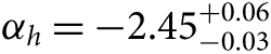
Since a universal IMF cannot have a high-mass slope that is steeper, flatter or equal to the Salpeter value, the logical conclusion, then, is that the IMF is not ‘universal.’ The limitations in this argument will be clear, and it is obviously not a formal proof, but the conclusion that a growing wealth of evidence points against a ‘universal’ IMF is inescapable.
If the IMF is not universal, then authors must be wary of inconsistent usage of assumed IMFs. As a naive example, galaxy SFRs may be calculated assuming a nominal IMF, but then compared against SPS outputs assuming a variety of input IMFs in order to establish which (erroneously) better matches the data. Such analyses must be careful to ensure self-consistency of IMF assumptions throughout. This is true of cosmic census analyses as well.
If the IMF is not universal, then there are clearly many observational implications, that can be tested to further explore the extent of any IMF variation. For example, Ferreras et al. (Reference Ferreras, Weidner, Vazdekis and La Barbera2015) show that no single IMF with a fixed high-mass (m > 0.5 M⊙) slope (αh = −2.3) and a low-mass slope ranging from –2.8 ≤ αl ≤ –1.8 can reproduce the observational constraints from the stellar populations of massive early type galaxies, together with their observed metallicities. They conclude that an evolving IMF (Weidner et al. Reference Weidner, Ferreras, Vazdekis and La Barbera2013) is required to explain the joint constraint. Some implications of a varying IMF were explored by Clauwens, Schaye, & Franx (Reference Clauwens, Schaye and Franx2016), who show the impact of assuming the metallicity-dependent IMF found by Martín-Navarro et al. (Reference Martín-Navarro2015d) on the SFR of galaxies, the stellar mass function, mass–metallicity relation and reionisation. The results range from significant to minimal, depending on how the dwarf-to-giant ratio of the IMF is implemented, but define a clear set of observational constraints that can be used to begin ruling out particular IMF forms. The substantial variations in physical distributions seen for some of these comparisons, many already inconsistent with observation, highlight the significant existing scope to begin a focused program of quantifying any potential variation in the IMF.
As a thought experiment, consider whether the metallicity-dependent or σ-dependent ‘bottom-heavy’ IMF for spheroids (αl ≲ −2.35, m < 1 M⊙) and the SFR-dependent ‘top-heavy’ IMF for disk galaxies (αh ≳ −2.35, m > 0.5 M⊙) might both be consistent with the sense of a putative evolving IMF from the SFH/SMD constraint. We can use the two-phase model for the evolution of galaxies proposed by Driver et al. (Reference Driver, Robotham, Bland-Hawthorn, Brown, Hopkins, Liske, Phillipps and Wilkins2013). In this model, systems that will become spheroids dominate the SFH earlier (with a peak around 3 ≲ z ≲ 5) than those that become disks (with a peak around z ≈ 1). If the spheroids and disks of Driver et al. (Reference Driver, Robotham, Bland-Hawthorn, Brown, Hopkins, Liske, Phillipps and Wilkins2013) respectively have the ‘bottom-heavy’ and ‘top-heavy’ IMFs seen locally (as defined above), then in very qualitative terms, it would appear that the IMF evolution should be increasingly dominated by ‘bottom-heavy’ systems at higher redshift, inconsistent with the allowed evolution from the SFH/SMD constraint. Such a coarse analysis clearly neglects many effects that need to be investigated in more detail, but this illustration hopefully indicates the scope of opportunities for continuing to explore and refine our understanding of the IMF.
It might be argued, adopting the traditional approach, that all of the work above may be considered ‘consistent with a (poorly specified) universal IMF (with large uncertainties)’, given the variety of conflicting results, counter-claims, and limitations. I hope by this point that the specious nature of this conclusion is clear. There appears to be clear and growing evidence, albeit with a variety of associated limitations, for some degree of variation in the IMF, and it is appropriate for the conversation to move on to constraining such variations rather than dismissing them.
On that note, I briefly explore simulation work in Section 7, aiming to highlight the need for modelers to focus not on reproducing a particular IMF behaviour, but on identifying which physical conditions lead to what kind of IMF behaviour, and under what assumptions. Only by reframing the question to one that asks how the IMF varies and how do different assumptions or physical conditions impact such variation can we begin to make self-consistent progress in understanding the IMF itself.
7. IMF measurement approaches: simulations and models
7.1. Simulating star formation
The physics of star formation is an enormous field, and I do not pretend to provide a thorough review here. The purpose of the current summary is to highlight the complexity of the field, and the challenge in directly linking fundamental astrophysical processes to the form of an IMF. For details of work in this area, interested readers are referred to reviews by Krumholz (Reference Krumholz2014), and Offner et al. (Reference Offner, Clark, Hennebelle, Bastian, Bate, Hopkins, Moraux and Whitworth2014), work by Hopkins (Reference Hopkins2013a), Bate, Tricco, & Price (Reference Bate, Tricco and Price2014), Guszejnov & Hopkins (Reference Guszejnov and Hopkins2015), Bate & Keto (Reference Bate and Keto2015), Klishin & Chilingarian (Reference Klishin and Chilingarian2016), Guszejnov, Krumholz, & Hopkins (Reference Guszejnov, Krumholz and Hopkins2016), Guszejnov, Hopkins, & Krumholz (Reference Guszejnov, Hopkins and Krumholz2017), and references therein.
For ease of readability I refer below to ‘top-heavy’ or ‘bottom-heavy’ IMFs in reference to work that uses those terms. These correspond respectively to αh ≳ −2.35 (usually for m > 0.5 M⊙, sometimes α ≳ −2.35 for the full mass range) and αl ≲ −2.35 (often for m < 1 M⊙, but about as often also α ≲ −2.35 for the full mass range). Since this summary is largely qualitative, this usage should not be too ambiguous.
The recent work by Krumholz et al. (Reference Krumholz, Myers, Klein and McKee2016) provides a concise introduction to the key elements considered by most star formation simulations. In brief, the thermal Jeans mass, turbulence, magnetic fields, radiative feedback and mechanical feedback are all considered by various authors to play more or less significant roles. That analysis extends work by Krumholz (Reference Krumholz2011), who quantifies how radiative feedback can set the stellar mass scale, in turn building on earlier work by Bate (Reference Bate2009) and Krumholz (Reference Krumholz2006). He argues that radiative processes are the dominant mechanism in determining the gas temperature and ultimately the origin of the peak in the IMF.
Early work proposed an IMF characteristic mass determined by the thermal Jeans mass (e.g. Larson Reference Larson1998, Reference Larson2005). Being temperature dependent, this would lead naturally to higher mc in extreme environments such as super star clusters or galactic nuclei, or high redshift galaxies. Other potential drivers, such as the role of metallicity, have subsequently been explored. There are arguments that, while metallicity plays an important role in cooling for the formation of Population III stars, it is unlikely to have a direct effect on the IMF for later stellar generations (Bate Reference Bate2014, Reference Bate2005), apart from increasing the lower mass limit for lower metallicity systems. While Bate (Reference Bate2005) notes that metallicity may have an indirect impact because of its role in setting the Jeans mass during cloud fragmentation, to the degree that the Jeans mass of the cloud may affect the characteristic mass of the IMF, Bate (Reference Bate2014) find stellar mass functions that are consistent for metallicities ranging from 1/100 to 3 times solar. Similarly, using two numerical simulations corresponding to Jeans masses different by a factor of three, Bate & Bonnell (Reference Bate and Bonnell2005) argue that any potential IMF variation appears through a change in the characteristic mass of the system rather than a change in slope at the high-mass end.
It is clear that there is enormous complexity and interplay of the astrophysical processes involved in star formation. Given this complexity, it is easy to understand that a ‘universal’ IMF is an attractive end-state to aim at achieving with models and simulations, as a form of validation. Introducing IMF variations removes this touchstone, making the work of the theorists more challenging, but as the observational constraints become more complex, so too do the models in their efforts at addressing them. This has led in more recent work to the goal of testing how particular models fare in reproducing the range of popular published IMF variations.
Hopkins (Reference Hopkins2013b) uses the excursion set formalism to calculate mass functions from the density field in a supersonically turbulent interstellar medium. This analysis predicts that IMF variations are most likely to appear at the low-mass end, with remarkably uniform slope for high masses, for reasonable choices of temperature, velocity dispersion, and gas surface density. A different approach, based on a Press–Schechter formalism, by Hennebelle & Chabrier (Reference Hennebelle and Chabrier2013), extends their earlier work by including time dependence and the impact of magnetic field, and reaches similar conclusions. Chabrier, Hennebelle, & Charlot (Reference Chabrier, Hennebelle and Charlot2014) show how the turbulent Jeans mass leads to the peak of the IMF shifting towards lower masses, to reproduce ‘bottom-heavy’ IMF shapes. Subsequently Bertelli Motta et al. (Reference Bertelli Motta, Clark, Glover, Klessen and Pasquali2016) identified conditions in two suites of hydrodynamic simulations that lead to IMF variations at the high-mass end. Recently, though, Liptai et al. (Reference Liptai, Price, Wurster and Bate2017) have argued against supersonic turbulence being the primary driver in the shape of the IMF, based on two sets of simulations with different turbulent modes, finding statistically indistinguishable differences in the resulting IMFs.
It seems that despite the growing sophistication of our theoretical understanding of star formation, there is still scope for refinement in identifying the various dominant physical mechanisms in different astrophysical environments. Elmegreen (Reference Elmegreen, Kang, Lee, Leung and Cheng2007) notes that ‘most detailed theoretical models reproduce the IMF, but because they use different assumptions and conditions, there is no real convergence of explanations yet’. In the subsequent decade, although the models have become more sophisticated, subtle and complex, so have the observational constraints, and the outcome remains largely the same.
7.2. Simulating galaxy evolution
Moving from the complexity of astrophysical processes in individual star formation to the larger scale of galaxies requires a different form of modelling and simulations. As above, this is a vast field in its own right, and only briefly and incompletely summarised here with the aim of identifying some of the developments and challenges.
Galaxy populations are typically modelled through semi-analytic recipes embedded in large cosmological simulations, and individual or small numbers of galaxies through detailed hydrodynamical simulations with better physical resolution than the cosmological models. In the absence of confirmed physical drivers underlying the shape of the IMF, such simulations tend to invoke a range of empirical or phenomenological relations that have some physical motivation. The outcome is that most observational evidence for IMF variations is able to be reproduced by a suitable choice of physical dependencies for the IMF, although not all results are consistent with each other, or necessarily self-consistent.
Baugh et al. (Reference Baugh, Lacey, Frenk, Granato, Silva, Bressan, Benson and Cole2005) modelled the abundance of Lyman break galaxies and submillimetre galaxies, successfully reproducing luminosity functions and the optical and infrared properties of local galaxy populations, but found a need for a ‘top-heavy’ IMF to reproduce the observed 850 μm galaxy number counts. Without such a change to the IMF in the model, the constraint from the global SFR density led to the predicted number counts being too low. Allowing the IMF to be ‘top-heavy’ increases the 850 μm flux for a given (lower) SFR because of the relative increase in the number of high-mass stars, allowing the model to consistently reproduce both the number counts and the SFR density. Narayanan & Davé (Reference Narayanan and Davé2012) explore the impact of allowing mc to scale with the Jeans mass in giant molecular clouds, showing that this simple assumption leads to a reduction in the SMH/SMD discrepancy, as well as reducing the tensions in several other observational constraints. Narayanan & Davé (Reference Narayanan and Davé2012) extend this work to show that such an assumption leads to galaxies experiencing both ‘top-heavy’ and ‘bottom-heavy’ IMFs at different stages of their evolution, with the bulk of stars forming in a ‘top-heavy’ phase. Marks et al. (Reference Marks, Kroupa, Dabringhausen and Pawlowski2012) use a model of rapid gas expulsion to produce more ‘top-heavy’ IMFs in systems with increasing density and decreasing metallicity. Bekki (Reference Bekki2013a) shows that such density and metallicity dependencies for the IMF can lead, among other effects, to lower SFRs than with a fixed IMF, and that [Mg/Fe] is higher for a given metallicity. Similarly, Bekki & Meurer (Reference Bekki and Meurer2013) are able to reproduce the ‘top-heavy’ IMF results of Gunawardhana et al. (Reference Gunawardhana2011) by allowing the IMF to depend on local densities and metallicities of the interstellar medium. In contrast, Bekki (Reference Bekki2013b) show that ‘bottom-heavy’ IMFs can also be reproduced with suitable choices of metallicity and gas density in the star-forming gas clouds.
Taking a different approach, Fontanot (Reference Fontanot2014) uses a semi-analytic model to test the impact of different IMF prescriptions, broadly falling into two classes of SFR-dependent ‘top-heavy’ models and stellar mass-dependent or σ-dependent ‘bottom-heavy’ models. He finds that the ‘bottom-heavy’ models lead to variations in stellar mass and SFR functions similar to the uncertainty in the determination of those quantities, while the ‘top-heavy’ models lead to an underestimate in the high-mass end of the galaxy stellar mass function, compared to a fixed Kroupa (Reference Kroupa2001) IMF.
Blancato, Genel, & Bryan (Reference Blancato, Genel and Bryan2017) also explore the impact of observed IMF variations on models. They implement various IMF dependencies by tagging stellar particles in their simulation with individual IMFs using observationally derived dependencies on velocity dispersion, metallicity or SFR. They then find that the IMFs recovered in the simulated z = 0 galaxies no longer reproduce the imposed relations. This leads them to conclude that even more extreme physical IMF relations for some stellar populations are required to reproduce the observed level of variation. Sonnenfeld, Nipoti, & Treu (Reference Sonnenfeld, Nipoti and Treu2017) explore the evolution of αmm (defined here as the ratio of the true stellar mass to that inferred assuming a Salpeter IMF) using cosmological N-body simulations. They find that dry mergers do not strongly impact the relation between αmm and σ. They note, though, that the underlying dependence of the IMF on stellar mass or σ is mixed through the dry merger process, making it observationally challenging to infer which quantity was originally coupled with the IMF. Schaye et al. (Reference Schaye2010) tested the impact of a ‘top-heavy’ IMF at high gas pressures, finding that it reduced the need to invoke self-regulated feedback from accreting black holes to reproduce the observed decline in the cosmic SFR density at z < 2. Gargiulo et al. (Reference Gargiulo2015) argue that a ‘top-heavy’ IGIMF best reproduces the [α/Fe]-stellar mass relation for elliptical galaxies when there is an SFR-dependence for the IGIMF slope. Fontanot et al. (Reference Fontanot, De Lucia, Hirschmann, Bruzual, Charlot and Zibetti2017) also explore the implications of the IGIMF method in their semi-analytic model, finding that it leads to a more realistic [α/Fe]-stellar mass relation than with a fixed IMF.
It is clear that numerical simulations and semi-analytic models can provide valuable insights into the way we understand the IMF. In particular, they can be used to test how different physical prescriptions for star formation manifest, and the properties of the observational constraints on IMFs that they produce, as well as what accessible observational tracers give the most discrimination in measuring the IMF. It is important that models are used to make predictions for how different IMF prescriptions should present observationally, defining observational tests to refine or rule out particular forms of physical dependencies or underlying variation. There is perhaps more value in using the models in this way than merely through tweaking some underlying dependencies to reproduce a select subset of observational constraints. Because of the fundamental nature of the IMF it is important that models and simulations are used to test as broad a suite as possible of observational implications, rather than merely focusing on one or two in particular. This is to ensure that some observational constraints are not violated in the models while attempting to assess the impact on others.
Large cosmological hydrodynamical simulations are now available, such as Eagle (Schaye et al. Reference Schaye2015), Illustris (Vogelsberger et al. Reference Vogelsberger2014) and Magneticum (Dolag Reference Dolag2015) within which detailed galaxy simulations can be created, for example. By selecting sub-volumes sampling a broad range of galaxy environments and re-simulating those subregions at high resolution, it should be possible to identify the impact of different simulated IMFs on the physical properties of the resulting galaxies. Simulation outputs should be produced that are directly comparable to observables (e.g. luminosities as well as stellar masses or SFRs) to avoid the need to reconstruct such derived properties from observational data sets, and potentially introducing inconsistent assumptions regarding the IMF in doing so. By incorporating population synthesis approaches that link directly to the observational metrics being used in inferring IMF properties, there may be the opportunity to directly assess how underlying IMF dependencies are subsequently quantified observationally.
In summary, there is an opportunity to begin linking the numerical, semi-analytic and population synthesis model approaches to self-consistently assess whether observational approaches for inferring IMFs are actually providing the quantitative conclusions expected, or whether other underlying effects may dominate.
8. A consistent approach
8.1. IMF constructs
The IMF has been used as a tool in a broad range of different contexts, as illustrated above. But if the IMF is not universal, then the quantity actually being measured in these different contexts is not necessarily the same. When inferring an IMF based on the integrated light from a galaxy, the quantity being measured is not the same as when inferring an IMF from star counts or luminosity functions. Likewise, when using a cosmic census approach such as the SFH/SMD constraint, the quantity in question is different again.
Such spatial dependence of the IMF has been recognised since the earliest work, with Salpeter (Reference Salpeter1955) describing the IMF as ‘the number of stars in [a given] mass range … created in [a given] time interval … per cubic parsec’. The spatial dependence, though, can easily be glossed over, and especially with the idea of a ‘universal’ IMF guiding the thinking, it is easy to conflate IMFs associated with different spatial volumes (star clusters, galaxies) and treat them as the same entity when they may well not be. This can lead to artificial or apparent inconsistencies that may not necessarily be in conflict.
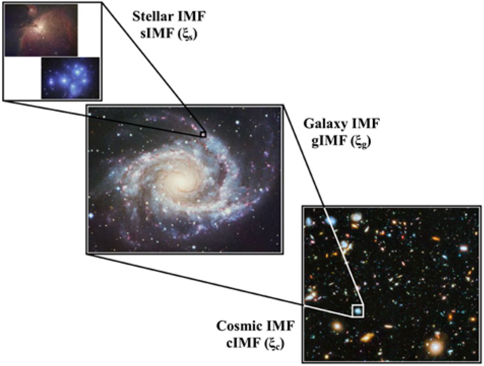
Figure 7. A framework to aid in clarifying discussions of the IMF. If the IMF is not universal, then the sIMF, gIMF, and cIMF are not necessarily the same, and all may have a time dependence. Different measurement techniques and observational samples probe these different quantities, and what has been referred to uniformly in published work to date as ‘the IMF’ conflates these distinct properties. This may well contribute to much of the current tension between different IMF estimates in different contexts.
The notion that the IMF within a star-forming region is potentially a different quantity than the effective IMF for a galaxy, and different again from the effective IMF for a population of galaxies at a given epoch, is an important foundational concept. Here I define these three quantities as the ‘stellar IMF’ or sIMF (ξs), the ‘galaxy IMF’ or gIMF (ξg), and the ‘cosmic IMF’ or cIMF (ξc) as illustrated in Figure 7. Lower case prefixes and subscripts are chosen here explicitly with the aim of minimising ambiguity between other commonly used variants such as IGIMF (for a galaxy-wide IMF), or CIMF (the cluster IMF for stellar clusters, or ‘core’ IMF for dense gas cores).
We can generalise the formalism of the IMF by writing the dependence on time and spatial volume explicitly:
 \begin{equation} \xi (m,t,V) = {{{\rm{d}}N(m,t,V)} \over {{\rm{d}}m{\kern 1pt} {\rm{d}}t{\kern 1pt} {\rm{d}}V}}, \end{equation}
where dN is the number of stars in mass interval dm created in the time interval dt within the spatial volume dV. In this generalisation it is important to note that the time dependence explicit to ξ allows for the form of the IMF to vary with time. It is different from the time-dependent mass function scaling that arises from a varying SFR, as defined, for example, by Schmidt (Reference Schmidt1959).
This approach describes the number of stars of a given mass that have formed up to a given time, for some spatial volume. Over a (short) finite time period and (small) spatial volume this is identically the stellar mass function (not accounting for stellar evolution):
 \begin{equation} \int_V \int_t \xi (m,t,V){\rm{d}}t{\kern 1pt} {\rm{d}}V = {\rm{d}}N(m)/{\rm{d}}m \end{equation}
and corresponds to what might be considered as a ‘traditional’ IMF. This approach eliminates the ambiguity between a nominal, or Platonic ideal, IMF from which real star clusters must be populated, and the actual instantiated mass function, since what is defined here is the real physical quantity of interest, the number of stars formed as a function of mass, time and location. The ‘universal’ IMF scenario can arguably be recovered by asserting that ξ has no temporal or spatial dependence, ξ(m) = dN(m)/dm, but this reopens the issue of accounting for a finite duration for star formation, and the effects of stellar evolution, since such a ξ(m) is in principle never observable (e.g. Kroupa et al. Reference Kroupa, Weidner, Pflamm-Altenburg, Thies, Dabringhausen, Marks and Maschberger2013). In contrast, ξ(m,t,V) is directly observable in principle, although in practice doing so may be highly challenging.
Integrating ξ(m,t,V) over different volumes gives the (time dependent) sIMF, gIMF and cIMF:
 \begin{equation} {\xi _s}(m,t) = \int_{{V_s}} \xi (m,t,V){\rm{d}}V = {\left[ {{{{\rm{d}}N(m,t,V)} \over {{\rm{d}}m{\kern 1pt} {\rm{d}}t}}} \right]_{{V_s}}}, \end{equation}
where Vs is a volume characteristic of a star-forming region, for example. Relations for ξg and ξc are analogous.
Clearly there must be a lower limit to the spatial scale or volume over which an IMF is a well-defined quantity, since it makes little sense to attempt to define an IMF at the scale of individual stars, for example. A natural minimum spatial scale is that sufficient to encompass a star cluster, and much of the work on the IMF focuses on the properties of stellar clusters or uses them to probe the IMF (as reviewed by, e.g. Bastian et al. Reference Bastian, Covey and Meyer2010). Also, the volumes referred to here are not specific fixed or comoving volumes in space (although they could be defined as such, in a numerical simulation, for example), but refer instead (for convenience) to a particular spatial scale, and which I illustrate through these three representative characteristic scales.
Considering the time dimension too is a revealing mental exercise. The process of star formation is not instantaneous. As stars form within a nascent star cluster there will be different mass functions extant depending on the time step sampled (e.g. Kroupa et al. Reference Kroupa, Weidner, Pflamm-Altenburg, Thies, Dabringhausen, Marks and Maschberger2013). There is an extensive literature on the protostellar mass function, explicitly to understand this time dependence in the way that the IMF is generated. McKee & Offner (Reference McKee and Offner2010), for example, present a formalism using models for mass accretion by protostars to link the IMF to its progenitor protostellar mass function, extended to the protostellar luminosity function by Offner & McKee (Reference Offner and McKee2011). A more recent analytic model for the mass gained by protostars is presented by Myers (Reference Myers2014). Hartmann, Herczeg, & Calvet (Reference Hartmann, Herczeg and Calvet2016) review accretion onto pre-main-sequence stars, and their Figure 13 highlights the different stellar mass and luminosity functions expected based on different accretion models.
For a large ensemble of clusters, throughout a galaxy say, each at a different stage in its formation process, the stellar mass function sampled over the full ensemble at a given time step may more closely resemble the mass function expected from a well-defined physical process, such as gravo-turbulent models (e.g. Hennebelle & Chabrier Reference Hennebelle and Chabrier2013; Hopkins Reference Hopkins2013b), although the mass function for any individual region may well be rather different, due to the complex feedback effects from stellar evolution during the formation event itself, and the local environment which may be influenced by adjacent regions of star formation or other astrophysical processes.
In this way of thinking, if there is a ‘universal’ physical process that drives star formation, then it is likely to be better sampled on the scales of galaxies (the gIMF) than within individual star-forming regions. Extending this idea, and to account for the possibility of variations between galaxies (due to a range of metallicities, star formation environments, and so on), any ‘universal’ physical process might be most accurately sampled through the effective stellar mass function over an entire galaxy population (the cIMF). This leads to the need for the physical processes of star formation to be able to explain potential variations in the stellar mass function from the scale of star clusters to galaxies (which may arise through effects unrelated to the star formation process itself), ultimately converging on a model prediction when sampled over sufficiently large regions. This may be written as ξ(m,t) = ∫V ξ(m,t,V)dV→IMF for V→Vc where Vc is some large volume encompassing one or more galaxies, and ‘IMF’ here is being used to describe the stellar mass function expected from a nominal ‘universal’ physical process.
As an alternative, rather than the sampling of a large spatial volume at a fixed time step, a small volume may be considered over a long period of time to equally ensure that all phases of the physical process of star formation are sampled. This might be summarised as ξ(m,V) = ∫tξ(m,t,V)dt→IMF for t→t c where t c is large compared to the duration of a star formation event, perhaps capturing multiple such events within the volume V, and ‘IMF’ is used as above. Observationally this is not a practical approach, while the former is, but it may be of value in simulations.
This is another way of considering the arguments posed by Kruijssen & Longmore (Reference Kruijssen and Longmore2014), as this concept equally applies to the gas clouds from which the stars are forming, and the associated ‘core’ mass functions, or the mass functions of stellar clusters. Any given gas reservoir may not be representative of the full population of star-forming gas clouds throughout a galaxy, and only by sampling a sufficient number of them will the statistics of the density distribution be accurately represented.
8.2. Linking mass functions between different spatial scales
With differing stellar mass functions on different spatial scales, a natural question arises regarding how to relate individual mass functions on small scales to those measured on the larger scales, i.e., how to link the sIMF for multiple star-forming regions to the gIMF for the galaxy comprising those stars. The IGIMF method (Kroupa & Weidner Reference Kroupa and Weidner2003; Weidner & Kroupa Reference Weidner and Kroupa2005; Kroupa et al. Reference Kroupa, Weidner, Pflamm-Altenburg, Thies, Dabringhausen, Marks and Maschberger2013) is one approach, which broadly speaking considers a summation of many sIMFs to construct the gIMF. This method assumes that stars form in self-regulated embedded clusters, which follow a relationship between the total mass of a stellar cluster and the mass of its highest mass star. Their sIMFs are therefore empirically constrained by the stellar cluster mass. They can be summed to calculate the gIMF, or the IMF of a region within a galaxy containing multiple stellar clusters, and can lead to a variable gIMF (Yan et al. Reference Yan, Jerabkova and Kroupa2017). This approach allows a gIMF to be calculated given a knowledge of how the sIMF depends on the physical conditions of star formation. The early results using this technique favoured galaxy-wide IMF slopes somewhat steeper at the high-mass end than that of the individual star-forming regions. Later work incorporating constraints on the variation of the sIMF from Marks et al. (Reference Marks, Kroupa, Dabringhausen and Pawlowski2012) extended this approach to show how flatter IGIMF slopes at the high-mass end could be produced in galaxies with high SFRs (Yan et al. Reference Yan, Jerabkova and Kroupa2017).
The way that sIMFs themselves arise, or their dependencies on associated astrophysical processes, may differ from the IGIMF assumptions. Some level of variation would seem likely given that star formation happens in a complex multiphase medium, with regions of star formation potentially overlapping, and triggering or suppressing one another in highly non-linear ways, all of which may evolve with time. So the gIMF may not necessarily comprise a sum over a discrete set of identical, or even simply modelled sIMFs. If each such star formation event can be characterised by its own sIMF, though (whether or however it is influenced by, or overlapping with, neighbouring events) we can write
 \begin{equation} {\xi _g}(m,t) = \int_{{V_g}} {\xi _s}(m,t,V){\rm{d}}V, \end{equation}
where Vg is the volume of the galaxy in question. It is important to distinguish this generalisation from the IGIMF method, since in the current approach each ξs(m, t, V) may arise from different physical dependencies or processes to those assumed in the IGIMF approach.
Likewise, the cIMF may be able to be approximated as a simple sum over gIMFs. Of course, galaxy interactions are an important channel for galaxy evolution, and they are clearly associated in many cases with significant levels of star formation. But assuming for the present argument that stars formed in this mode are a negligible fraction of all stars formed, or alternatively can be accounted for through separate characterisation with their own ξg(m, t, V) we can write
 \begin{equation} {\xi _c}(m,t) = \int_{{V_c}} {\xi _g}(m,t,V){\rm{d}}V, \end{equation}
where Vc is the cosmic volume being probed.
In this formalism there is no analogue to the process of generating a stellar mass function by ‘populating’ or ‘drawing from’ some underlying IMF, since ξ(m,t,V) here is in effect the stellar mass function itself, incorporating its spatial and temporal variations. Instead, the link to be highlighted is over what spatial or temporal scales this mass function needs to be sampled in order to compare with predictions from various physical models of star formation. In this context, questions such as whether the sIMF is drawn from a gIMF, or how to ‘populate’ an sIMF, are poorly posed, and not helpful in developing our understanding of star formation.
8.3. Derived quantities
The SFR and total stellar mass are directly linked to the IMF (e.g. Schmidt Reference Schmidt1959), and there is some value in presenting this explicitly. The SFR, S(t,V), is the mass of stars formed in a time interval dt and volume dV:
 \begin{equation} S(t,V) \equiv {{{\rm{d}}m} \over {{\rm{d}}t}}(t,V) = \int_{{m_l}}^{{m_u}} m\xi (m,t,V){\rm{d}}m, \end{equation}
and the total mass in stars ever formed in that volume over some time period t 1 to t 2 is then:
 \begin{equation} \eqalign{ {m_{total}}(V) & = \int_{{t_1}}^{{t_2}} S(t,V){\rm{d}}t \\ & = \int_{{t_1}}^{{t_2}} \int_{{m_l}}^{{m_u}} m\xi (m,t,V){\rm{d}}m{\kern 1pt} {\rm{d}}t. \cr} \end{equation}
The mass remaining in stars at a time τ is mτ = (1–R)mtotal, where R is the mass recycled into the interstellar medium (ISM) due to stellar evolutionary processes, and is dependent on the stellar mass distribution. Recycling fractions can be calculated for a given mass distribution if the mass returned to the ISM is known as a function of initial stellar mass (e.g. Renzini & Voli Reference Renzini and Voli1981; Woosley & Weaver Reference Woosley and Weaver1995). This is also expected to depend on metallicity.
8.4. Implementation
The value of a ‘traditional’ IMF is largely through the ability to use it as a tool to infer the presence of stellar populations not directly observed. Depending on the techniques being used, observables are often limited either to the high-mass (e.g. through Hα, UV, or infrared tracers) or the low-mass (e.g. direct star counts, or gravity sensitive spectral features) range of the stellar mass distribution, and accounting for the stellar populations not directly measured is done by invoking an IMF. With an assumed ‘universal’ IMF simply characterised through a well-defined parametric form, such extrapolations are straightforward.
In the general case posed above, a number of simplifying assumptions need to be incorporated in order to regain the utility of the simple ‘universal’ model. The value of the general approach is that these assumptions now become explicit, rather than implicit, defining the form (or absence) of any temporal or spatial variations (which may reflect other underlying physical dependencies). The same parameterisations (incorporating physical dependencies if desired) can be applied as always, using the general formalism, but assumptions about the spatial scale or epoch to which such parameterisations apply become clear. This hopefully enables distinctions to be drawn between stellar mass functions that should not necessarily be compared directly, to avoid artificial inconsistencies. It should also facilitate the exposing of internal contradictions within analyses.
The mass functions as parameterised by, say, Kroupa (Reference Kroupa2001) and Chabrier (Reference Chabrier2003a) are not inconsistent with this approach, and they can now be explicitly defined as the integrals over some spatial and temporal scale. So, to the degree that these Milky Way stellar mass functions (IMFMW) correspond to star formation on the scale of star clusters over a period of several Myr, we may write, for example, 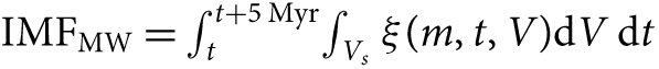 $ {\rm{I}}M{F_{MW}} = \int_t^{t + 5{\kern 1pt} {\rm{M}}yr} \int_{{V_s}} \xi (m,t,V){\rm{d}}V{\kern 1pt} {\rm{d}}t $, where Vs is the volume sufficient to encompass the star cluster, and 5 Myr is nominally taken as a timescale sufficient to allow the full range of masses for all stars to form. When exploring potential physical dependencies for a stellar mass function, the various observational constraints can be used in this fashion as boundary conditions.
8.5. A broader context
This more general approach can help in setting the context for the broader range of work on the IMF. In particular, by making explicit the potential spatial and temporal dependencies, which are likely a consequence of any underlying physical dependencies, the scales over which certain observational constraints apply also become explicit. It also means that analyses can be clear about the spatial and temporal scales for the stellar mass functions they are using, or making predictions for. For example, the investigation of Blancato et al. (Reference Blancato, Genel and Bryan2017) adopts an observed gIMF, which is then implemented as an sIMF in simulations. They find, perhaps not surprisingly given the discussion above, that this does not lead to the observed gIMF being reproduced in the simulated galaxies, concluding that sIMFs need to be more extreme than adopted in order to replicate the observed gIMF.
The approach presented here provides the potential for self-consistent explorations in models and simulations, enables a clearer link between what the models predict and what the observations measure, and avoids conflation between constraints that apply to different physical scales. It provides a framework in which the subtle biases associated with an implicit tendency towards a ‘universal’ IMF are eliminated, allowing for a more critical evaluation of the constraints on potential variations between stellar mass functions, and their link to the underlying physics of star formation.
With these considerations at hand, I now revisit the variety of observational constraints discussed above and position them in this self-consistent framework, in order to re-examine the extent to which the IMF may vary.
9. Discussion
9.1. What do the observations really tell us?
With the extensive sets of measurements, inferences and constraints summarised above, it is helpful in the discussion of the degree of consistency or otherwise to present the results separately for the cIMF (ξc), gIMF (ξg), and sIMF (ξs), to ensure only comparable quantities are being examined. For the Milky Way and nearby galaxies, it may be possible to show these in diagrams representing each of ξg and ξs depending on whether the full galaxy, or star-forming regions within it, are shown. This consideration also reveals a distinction between ‘field star’ IMFs and those for stellar clusters, since the ‘field stars’ probe, in a sense, the gIMF, while the stellar clusters probe the sIMF.
It quickly becomes clear when doing this that many published IMF constraints are actually not directly comparable, and that, in fact, there is an extensive range of parameter space to explore in addressing the question of how to characterise the IMF. In the following figures, representative regions are shown for simplicity and by way of illustration, rather than attempting to reproduce individual measurements in detail, especially because in some cases they are not available, although a range of IMF slopes has been given.
In the presentation here I focus on comparisons of IMF shapes as characterised generally by the low- and high-mass slopes, αl and αh, largely because that is the most common approach taken in the published work. In many cases, though, it may be possible to explain the observed results by a different approach to modifying the IMF shape, such as an increase in mc rather than a more positive (flatter) value of αh, or reducing mu rather than a more negative (steeper) value of αh, for example. Other measures, too, such as αmm, will be important to include in the development of a suite of diagnostic diagrams for constraining the measurement of the IMF. These points should be borne in mind when considering the discussion below.
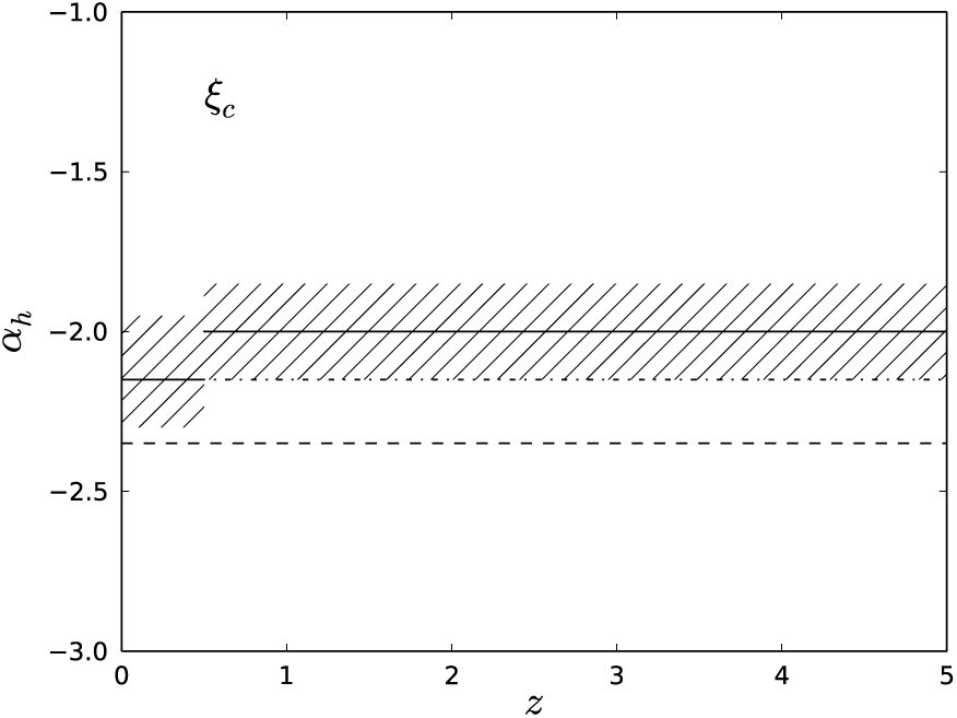
Figure 8. The possible variation in αh for ξc from Wilkins et al. (Reference Wilkins, Hopkins, Trentham and Tojeiro2008b) (solid lines and hatched regions). The dashed line is the Salpeter slope (αh = −2.35) and represents the ‘universal’ IMF from Madau & Dickinson (Reference Madau and Dickinson2014). The dot-dashed line is αh = −2.15 from Baldry & Glazebrook (Reference Baldry and Glazebrook2003).
There are relatively few observations inferring ξc, illustrated in Figure 8, and only αh is typically constrained. A value for αl as steep as Salpeter is ruled out (e.g. Hopkins & Beacom Reference Hopkins and Beacom2006; Madau & Dickinson Reference Madau and Dickinson2014), but most analyses then assume αl = −1.3 (Wilkins et al. Reference Wilkins, Hopkins, Trentham and Tojeiro2008b) or αl = −1.5 (Baldry & Glazebrook Reference Baldry and Glazebrook2003; Hopkins & Beacom Reference Hopkins and Beacom2006) to be consistent with that for the Milky Way. Figure 8 shows the Salpeter slope from Madau & Dickinson (Reference Madau and Dickinson2014), αh = −2.15 from Baldry & Glazebrook (Reference Baldry and Glazebrook2003), and the evolving high-mass slope of Wilkins et al. (Reference Wilkins, Hopkins, Trentham and Tojeiro2008b). The ‘paunchy’ IMF from Fardal et al. (Reference Fardal, Katz, Weinberg and Davé2007) is not shown, as there are multiple αh values (the slope is different for different mass ranges above m > 0.5 M⊙, see Section 6), but these values bracket those shown in Figure 8. The relatively small variation seen in αh demonstrates the potential of the cosmic census approaches in strongly constraining ξc. Already variations in αh for ξc at the 10% level are potentially being discriminated between, and future constraints will be even tighter. It seems fairly clear from this comparison, though, that if the cIMF does evolve, the extent of any evolution needed to resolve the SFH/SMD constraint is relatively mild, and at the level of 10−20% in αh.
The gIMF has constraints on αh for the star-forming population, and on αl for the passive population, but there is no real overlap between the two. The studies constraining αh are not sensitive to αl and vice versa. Figure 9a shows, as an illustration, the range of values for αh from Meurer et al. (Reference Meurer2009), Gunawardhana et al. (Reference Gunawardhana2011) and Nanayakkara et al. (Reference Nanayakkara2017) as a function of redshift, compared with that for the Milky Way (e.g. Kroupa Reference Kroupa2001) and M31 (Weisz et al. Reference Weisz2015). The results of Nanayakkara et al. (Reference Nanayakkara2017) at high redshift may well extend to include steeper values, αh < −2.35, although the focus in their discussion is on the possibility of flatter slopes for the extremely high Hα equivalent width systems measured. The dependence of αh on galaxy properties is illustrated in Figure 9b, shown as a function of ΣHα, as inferred from Gunawardhana et al. (Reference Gunawardhana2011), Meurer et al. (Reference Meurer2009), and Nanayakkara et al. (Reference Nanayakkara2017). The relation of αh with ΣSFR from Figure 13 of Gunawardhana et al. (Reference Gunawardhana2011) has been converted to one with ΣHα using their SFR conversion factor (their Equation 5). Combining information from Figures 3 and 10b of Meurer et al. (Reference Meurer2009), we can infer the range of αh as a function of ΣHα to compare with the results of Gunawardhana et al. (Reference Gunawardhana2011) in Figure 9b. The Hα SFR from Figure 21 from Nanayakkara et al. (Reference Nanayakkara2017) can be used, with an assumed galaxy size of approximately 3–4 kpc (Allen et al. Reference Allen2017), and the range of αh inferred from their earlier figures to reconstruct a rough estimate of how their data may populate this relation.
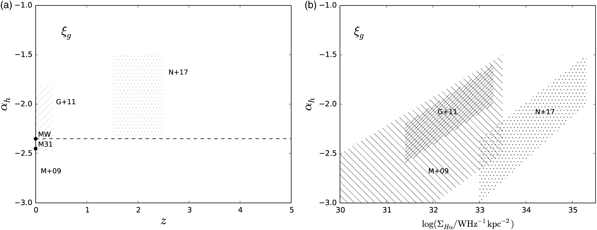
Figure 9. (a) The possible variation in αh for ξg from Meurer et al. (Reference Meurer2009), Gunawardhana et al. (Reference Gunawardhana2011), and Nanayakkara et al. (Reference Nanayakkara2017), shown as hatched and dotted regions. The dashed line is the Salpeter slope (αh = −2.35). Values for the Milky Way (MW) and M31 (Weisz et al. Reference Weisz2015) are also shown. Note that the full range of αh is indicated, and the dependencies on sSFR or other physical property are not represented here. (b) The approximate dependence of αh on Hα surface density, inferred from each of Gunawardhana et al. (Reference Gunawardhana2011),Meurer et al. (Reference Meurer2009), and Nanayakkara et al. (Reference Nanayakkara2017).
The point made by Gunawardhana et al. (Reference Gunawardhana2011) is worth reiterating. They state that if an IMF-dependent SFR calibration were used this would have the effect of reducing the range in SFR probed, but would not change their conclusion of an SFR-dependence for αh, since the variation is monotonic and the ordering of the SFRs would not be affected. There is some scope for future work here to develop a self-consistent constraint on αh with SFR-related parameters.
The low-mass slope (αl) for ξg is illustrated as a function of redshift in Figure 10. While the galaxies or stars observed in order to infer these measurements are all at very low redshift, the results are shown at illustrative formation times for the stars being analysed, making the coarse assumptions that Milky Way field stars formed 5–10 Gyr ago, while the ages for the passive galaxy stellar populations are taken as approximately 9.5–12.3 Gyr. This approach is taken in order to begin unifying our picture for ξg. So, for example, at z ≈ 2 we have from Nanayakkara et al. (Reference Nanayakkara2017) a high-mass slope for at least some galaxies up to αh ≈ –1.5 (Figure 9a), with a low-mass slope for at least some galaxies of either αl≈−1.3 or αl ≲ −2.35. It is interesting to note that there do not seem to be any measurements having intermediate values for the low-mass slope of ξg. Observations seem to favour either αl ≳ −1.5 or αl ≲ −2.35. This may echo the bimodality in low-mass sIMF shapes implied from the M/L ratios for globular cluster systems from Zaritsky et al. (Reference Zaritsky, Colucci, Pessev, Bernstein and Chandar2014b). They argue that these are consistent with either α = −2.35 for 0.1 < m/M⊙ < 100 for the high M/L systems (similar to the results for passive galaxies from, e.g. Conroy & van Dokkum Reference Conroy and van Dokkum2012) and a Milky Way style (Kroupa et al. Reference Kroupa, Tout and Gilmore1993) IMF (with αl ≈ –1.3) for the low M/L systems.
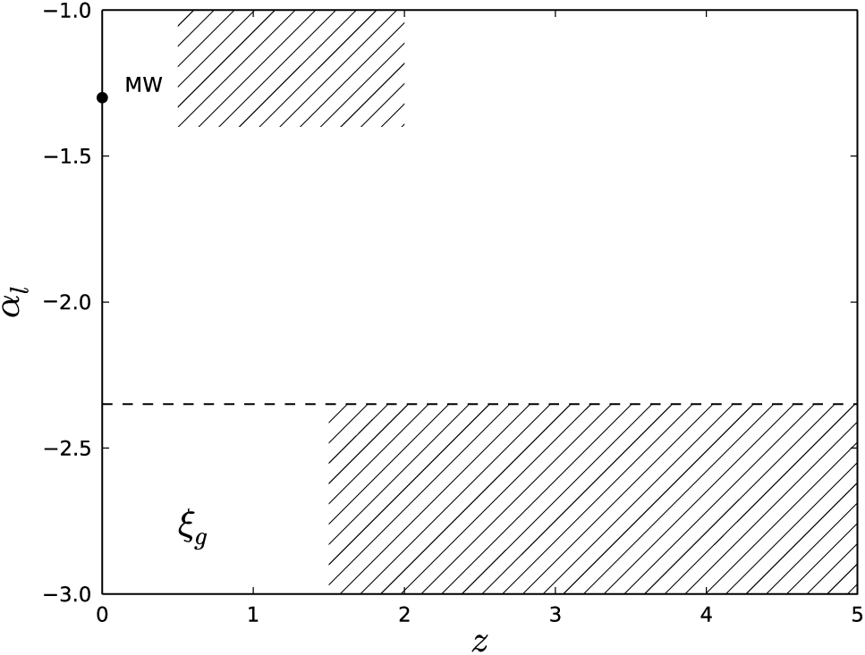
Figure 10. The low-mass slope of the IMF (αl) as a function of redshift, representative of the formation time of the stars involved. The Kroupa (Reference Kroupa2001) value for the Milky Way is shown as the data point, and the range of values for αl from Bastian et al. (Reference Bastian, Covey and Meyer2010) for Milky Way stars is shown as the upper hatched region, corresponding broadly to formation (lookback) times spanning 5≲t/Gyr≲10. The lower hatched region shows the steep low-mass IMF slopes, at formation times approximately 9.5≲t/Gyr≲12.3, for the passive galaxies discussed in Section 5.3. Note that the broad range of αl for these galaxies is indicated, and potential dependencies on σ or [M/H] are not represented.
The lensing, kinematic and dynamical constraints on the overall mass normalisation of the gIMF are harder to capture in these kinds of diagrams, as they do not give an explicit constraint on the gIMF shape, and the same mass normalisation can be achieved through various combinations of αl and αh (Section 5.3). In particular, some analyses for passive galaxies use a single power law gIMF to achieve a given mass normalisation, while others constrain αl = −1.3 and achieve the same mass normalisation through inferring a steeper αh. In the latter case, values as steep as αh ≈ −4 (e.g. Martín-Navarro et al. Reference Martín-Navarro2015c) are seen for galaxies observed at z ≈ 1 that have formation redshifts around z ≈ 2 (contrast with results shown in Figure 9a). As noted by Conroy (Reference Conroy2013), to retain a given gIMF mass normalisation, more positive (flatter) values for αh (such as those of Nanayakkara et al. Reference Nanayakkara2017) would imply a need also for more positive (flatter) values of αl, inconsistent with the more negative (steeper) values inferred for passive galaxies from the dwarf-to-giant ratio approach. In other words, the progenitors of low redshift passive galaxies must have had a gIMF different from that observed in situ in high redshift star-forming galaxies. This may be a further argument for a bimodality in the gIMF, possibly linked to the stellar M/L ratios for galaxies, that discriminates between spheroid and disk galaxy progenitors.
For the sIMF, ξs, it would be of interest to show αh and αl as a function of age, although here the effects of dynamical as well as stellar evolution would first need to be accounted for (De Marchi et al. Reference De Marchi, Paresce and Portegies Zwart2010). It would also be valuable to explore the sIMF parameters as a function of spatial scale, or total cluster mass, as well as stellar M/L ratio, to assess the potential for a link to ξg. With new telescopes such as the JWST and the GMT enabling the opportunity to explore ξs for more resolved stellar systems within nearby galaxies, it will be valuable to begin quantifying the range of physical parameters currently probed for existing stellar clusters and associations, in order that larger samples spanning a broader range of environments can be put in a common context. In particular, as the sample sizes grow for measuring ξs, there is an opportunity to begin to reduce the sampling errors and discriminate physical effects from sampling effects, in order to establish whether apparent differences between super star clusters, field stars or low SFR regions, and globular clusters are confirmed, and can be attributed to one or more specific physical processes.
The hope is that by discriminating explicitly between ξs, ξg and ξc, and beginning to explore each self-consistently through diagnostic diagrams such as those in Figures 8–10, and others that should easily be apparent, clear constraints on any IMF variations should be able to start being quantified.
9.2. Unifying our understanding of the IMF
It is possible to bring this complex suite of observational constraint and inference together by recasting astrophysical questions in this self-consistent approach. Larson (Reference Larson1998) presented a selection of evidence that argued for a ‘top-heavy’ IMF at early times. These included the G-dwarf problem, perhaps now updated as the CEMP star problem, and the evolution of the cosmic luminosity density. The first can now be cast as a constraint on the gIMF, and the second as a constraint on the cIMF (discussed in detail in Section 6). Importantly, such questions can now be addressed in a quantitative fashion, in order to establish whether any given gIMF, for example, can resolve both the CEMP star constraint and the Kennicutt diagnostic results from Hoversten & Glazebrook (Reference Hoversten and Glazebrook2008), Gunawardhana et al. (Reference Gunawardhana2011) and Nanayakkara et al. (Reference Nanayakkara2017). Similarly, such gIMFs can easily be assessed to see if they are consistent with the mass normalisation required for the low redshift passive galaxy population. The link between the gIMF and its contributing sIMFs must also be tested, to ensure consistency with the constraints from stellar clusters.
By bringing together the observational constraints in a tractable way, the issue can evolve from individual analyses identifying which IMF form best fits their data, to a set of constraints that must all be met by any successful IMF. This may or may not involve IMF variations, but a strong set of quantitative boundary conditions ensures that any limits on variations can be well measured.
The use of stellar M/L ratios as a unifying property is worth exploring given that it is a quantity that can be applied across a broad range of spatial scales. The similarity shown by Zaritsky et al. (Reference Zaritsky, Colucci, Pessev, Bernstein and Chandar2014b) for the two populations of globular clusters compared to the passive and disk galaxies is tantalising (Figure 2). There may still be a disconnect related to age, though, since the high ϒ* globular clusters tend to be those that are young, while the similar ϒ* passive galaxies have much older stellar populations. The situation is reversed for the low ϒ* globular clusters, which tend to be those with older stellar populations compared to the younger stellar populations with similarly low ϒ* in actively star-forming disk galaxies. Regardless, there is clearly scope to explore this link further.
It is perhaps worth postulating two broad scenarios at this stage, following from the suggestion above that there may be evidence for a bimodality in forms taken by the gIMF. Scenario 1 is the ‘bottom-heavy’ mode, characterised by α = −2.35 over 0.1 < m/M⊙ < 100, and possibly with even steeper αl<−2.35. This mode is that which seems to characterise passive galaxies and their progenitors, high ϒ* globular clusters, and possibly low surface brightness or low SFR dSph galaxies or star-forming regions. Scenario 2 is the ‘top-heavy’ mode, characterised by αh > −2.35 (with αl ≈ −1.3), that appears to be required for high SFR galaxies and star-forming regions, and possibly also at high redshift by the cosmic census constraints. It may not be the first time such a model has been proposed, but linking these broad scenarios directly and explicitly with the different sIMF, gIMF, and cIMF constraints will hopefully aid work on the underlying physics of star formation to help clarify which observations (how and in what conditions) the modelled or simulated instantiated mass functions need to be reproduced. A variety of models and simulations already exist that can reproduce such behaviour (see Section 7) in at least some circumstances, and the degree to which they self-consistently also reproduce other constraints needs to be tested.
9.3. Is the IMF universal?
I am hopeful that at this point we can dispense with this question as either misleading or poorly posed. The more relevant question is whether there is a ‘universal’ physical process for star formation. The IMF as a concept is perhaps better presented directly as the evolving and spatially varying stellar mass function explicitly, ξ(m,t,V) (Section 8). Clearly the observed stellar mass functions may vary dramatically between different stellar clusters, associations and galaxies, as a consequence of dynamical and stellar evolution and physical conditions. The stellar mass distribution on the scale of galaxies is not necessarily expected to be the same as that for a star cluster, nor that for a population of galaxies as a whole. There are numerous lines of evidence, summarised above, that the gIMF in particular may show two qualitatively different shapes. In order to assess this further, models and simulations should consider explicitly distinguishing between the IMF on different scales, testing and comparing against observations on appropriate scales. In particular, if there is a ‘universal’ physical process of star formation, that process must lead to the full range of IMF variations seen on the different scales and in the different contexts presented above.
9.4. Future work
There are many areas where work on understanding the IMF can be developed further, through simulations and observations, some of which are briefly touched on here. These opportunities are qualitatively different for the sIMF, gIMF, and cIMF although in all cases, presenting results in terms of IMF independent observables (such as luminosity) as well as derived (IMF dependent) quantities (such as masses and SFRs) is an important aid to clarity.
For the sIMF, especially where stellar systems need to be resolved, new telescopes such as JWST or the GMT will enable significant new breakthroughs. For the cIMF, there is an opportunity to update the review of Madau & Dickinson (Reference Madau and Dickinson2014) by conducting a critical assessment of the many published SFH and SMD measurements, and other cosmic census constraints like the extragalactic background radiation density and supernova rates. This is needed to develop a ‘gold standard’ reference set of observations to serve as the boundary conditions for any cosmic census approach.
As chemical abundance measurements are highly sensitive to the IMF, precision abundance measurements of a large population of stars can be used to improve such constraints. The GALAH survey (De Silva et al. Reference De Silva2015; Martell et al. Reference Martell2017) is one such project, to deliver precision chemical abundances for a million Milky Way stars, with currently about 0.5 million spectra in hand. Using the technique of ‘chemical tagging’ (Freeman & Bland-Hawthorn Reference Freeman and Bland-Hawthorn2002; Bland-Hawthorn & Freeman Reference Bland-Hawthorn and Freeman2004; De Silva et al. Reference De Silva, Freeman, Bland-Hawthorn, Asplund and Bessell2007; Bland-Hawthorn, Krumholz, & Freeman Reference Bland-Hawthorn, Krumholz and Freeman2010a), the preserved chemical compositions of stars allow the reconstruction of original star-formation events that have long dispersed into the Galaxy background, and possibly even the residual signatures of the first stars in the early universe (Bland-Hawthorn et al. Reference Bland-Hawthorn, Karlsson, Sharma, Krumholz and Silk2010b). In consequence, the large numbers of elemental abundances and large sample size measured by GALAH may enable the most robust measurement yet using this technique of the historical IMF of the Milky Way (G. De Silva, personal communication).
Measurements of the gIMF will continue to be able to draw on a wealth of observational data from existing and upcoming large survey programs, including the large integral field survey SAMI (Croom et al. Reference Croom2012; Green et al. Reference Green2018) and the Taipan galaxy survey (da Cunha et al. Reference da Cunha2017) that aims to obtain spectra and redshifts for around 2 million galaxies over the Southern hemisphere. The way the gIMF is measured relies heavily on SPS models, but at present different models are used in different contexts (passive galaxies are analysed one way, star-forming galaxies another). There is an opportunity to develop SPS models that can provide the information used in multiple IMF metrics self-consistently. This would allow, for example, the stellar absorption features used in the dwarf-to-giant ratio approach for an old stellar population to be linked directly to the Kennicutt diagnostics for that same stellar population at a younger age, in order to self-consistently assess a passive galaxy population and a star-forming galaxy population within a common framework.
Such advances in SPS modelling also need to incorporate the effects of stellar rotation and binarity or multiplicity in stellar systems. There is also an opportunity through new stellar surveys, such as GALAH (De Silva et al. Reference De Silva2015), to extend the range of metallicity and abundances used in stellar evolutionary libraries, on which the SPS models rely. More comprehensively spanning the observed range of stellar properties in this way would reduce the potential that inferred IMF properties might be a consequence of model systematics. This comes, though, at the cost of a greater range of model parameters which may not be observationally well-constrained, and will likely extend these areas of research in their own right.
There is scope to further explore mass-to-light ratio constraints self-consistently with the SPS approaches, by applying both uniformly to a well-defined set of stellar clusters and galaxies. Using both together can break the degeneracy in IMF shape arising from the mass-to-light ratio constraint alone. This approach could potentially lead to a method that links or even unites star cluster constraints with galaxy constraints.
With a field as broad and far-reaching as that of the IMF, there are clearly many more areas in which to pursue improvements in our understanding. Those listed here are just a few that may be valuable to address, directly arising from the discussion and considerations above.
10. Conclusions
The stellar IMF is a critical property influencing almost all aspects of star and galaxy evolution, and it has been the focus of a prodigious wealth of research spanning more than sixty years. This review has adopted a particular emphasis on the growing range of observational approaches to inferring or constraining the IMF, and exploring their strengths, weaknesses and apparent conflicts.
I have pedantically recommended that unambiguous terminology be adopted, echoing similar pleas dating back twenty years, and argued for the use of a standard nomenclature convention to minimise ambiguity (Sections 2.2 and 2.3).
I have explored the issue of a ‘universal’ IMF, and raised concerns about the Occam’s Razor default towards ‘universality’. This is accompanied by a recommendation that the most general scenario, that the IMF is not ‘universal’, rather than the simplest, be taken as the baseline assumption (Section 2.4). This baseline approach should lead to a clearer presentation in the literature around degrees of uncertainty and the physical parameter ranges being probed, to aid in defining the extent of any possible IMF variation.
Relying heavily on previous reviews where available, I have summarised results from a selection of studies that infer the IMF, spanning the scale of stellar clusters to galaxies and galaxy populations, along with simulations that model it (Sections 3–7). This was followed by the introduction of a general and self-consistent approach (Section 8). This approach makes the temporal and spatial dependencies of the stellar mass function explicit, ξ(m,t,V), leading to clear distinctions between ξs, ξg, and ξc representative of the spatial scale of stellar clusters, galaxies, and cosmic census probes of galaxy populations. These quantities should not in general be expected to be the same and should not be conflated or compared.
Using this self-consistent approach, a selection of new diagnostic diagrams were introduced to explore the IMF shapes from a selection of published results (Section 9), complementing and extending the ‘alpha plot’ (Scalo Reference Scalo, Gilmore and Howell1998; Kroupa Reference Kroupa2002; Bastian et al. Reference Bastian, Covey and Meyer2010). These diagnostics were used to assess the degree to which published IMF properties are consistent or not. If the cIMF evolves, the degree of evolution only needs to be mild in order to resolve the SFH/SMD constraint. The gIMF, in contrast, does seem to show some evidence for a bimodality in the IMF shape for star-forming galaxies and the progenitors of low redshift passive galaxies. There is scope now to begin presenting the many sIMF measurements in diagnostic diagrams similar to these in order to further quantitatively explore possible dependencies on a range of physical conditions.
This review has, inevitably, been limited in many ways. I have endeavoured to capture the current state of the field through summarising representative work, in order to tease out where tensions actually exist. I have presented a general approach that may be of value in supporting simulations and models to more precisely compare against the most relevant observational constraints. It is my hope that this review provides a unifying perspective for this fundamental aspect of the formation and evolution of stars and galaxies.
Author ORCIDs.
Andrew Hopkins http://orcid.org/0000-0002-6097-2747.
Acknowledgements
I am deeply grateful to Jill Rathborne for extensive discussion and invaluable support through the development and writing of this review. I thank the two anonymous reviewers for detailed and positive feedback that helped improve and refine the discussion presented here. My thanks also to Dennis Zaritsky, Madusha Gunawardhana, Pieter van Dokkum, and Michele Cappellari for their willingness to share the original versions of the figures from their papers that are reproduced here. I thank Pavel Kroupa for his careful reading of this lengthy work, identification of otherwise overlooked references, and his input in refining the descriptions of the IGIMF method. I greatly appreciate numerous conversations with Madusha Gunawardhana that have helped inform this review, and I thank her also for providing Figure 4. I thank Matthew Colless for input on this project, and his advice, mentoring, and guidance on many others over the past decade. I thank Warrick Couch for his valuable support in encouraging me to pursue this project and for enabling me to manage my time while working on this review. I gratefully acknowledge input as well from the following colleagues in helping to refine various different elements of this review: Joss Bland-Hawthorn, Elisabete da Cunha, Gayandhi De Silva, Chris Evans, Chris Power, and Ned Taylor.
I thank the Editorial Board of PASA for giving me the opportunity to contribute this work to the Dawes Review series. I have found it incredibly rewarding to explore the many areas and subtleties of this fascinating field, and it has been a privilege to share my perspective on this fundamental topic.


