


The Dawes Reviews are substantial reviews of topical areas in astronomy, published by authors of international standing at the invitation of the PASA Editorial Board. The reviews recognise William Dawes (1762–1836) (pictured in Figure 1), second lieutenant in the Royal Marines and the astronomer on the First Fleet. Dawes was not only an accomplished astronomer, but spoke five languages, had a keen interest in botany, mineralogy, engineering, cartography and music, compiled the first Aboriginal-English dictionary, and was an outspoken opponent of slavery.
‘Eppur si muove’
– Galileo Galilei (apocryphal)

Figure 1. William Dawes was a Royal Marine officer on the ‘First Fleet’ arriving in Australia in 1788. He was a man of many talents: engineer, map maker, botanist, and amateur astronomer. He was one of the first to document the Aboriginal Australian languages spoken in the Sydney region. He was the first person to make astronomical observations in Australia using telescopes from a place in Sydney Cove, now known as Dawes Point (Mander-Jones Reference Mander-Jones1966). Image Credit: miniature oil painting of Lieutenant William Dawes, 1830s, artist unknown. Collection: Tasmanian Museum and Art Gallery. Reproduced with their permission.
1 INTRODUCTION
The advent of new large telescopes coupled with new instrumentation technologies in the last decade has been extremely powerful in expanding our view of the high-redshift Universe. In particular, we have seen a flowering of the topic of high-redshift galaxy kinematics which studies their internal motions through high spatial and spectral resolution observations. The number of papers has exploded and we have seen a variety of surveys of observational approaches, analysis techniques, and theoretical interpretations. This has led to new paradigms of the nature of young galaxies but it has also raised problems in understanding as many new techniques have been used making comparison with the local Universe and traditional techniques difficult.
The Publications of the Astronomical Society of Australiahas decided to launch this new series of major reviews in honour of Lt. William Dawes. I have chosen to write it on the topic of these exciting new studies of the kinematics of high-redshift star-forming galaxies, one which has not had a major review and is in need of one. This is the first such Dawes review and as such there is no tradition to follow, instead one gets to set the tradition. I will choose to write this as a high-level introduction to the field, perhaps akin to the style of lecture notes, for the new worker in the field (for example an incoming postgraduate student). As such I will try and favour clarity and simplicity of explanations over totally complete lists of all possible references and ideas on a topic and will discuss analysis techniques in some detail. I will highlight the main surveys and the main ideas and warn in advance that some things may get left out. I will also allow myself the freedom to give more scientific speculation of my own than would occur in a traditional review; however, it will be clearly indicated what is a speculation. Obviously I will use the first person when needed as this seems appropriate for my approach.
1.1 Background and scope of this review
The rotation of the ‘spiral nebulae’ was one of the earliest and most fundamental observations of their nature and the second important discovery from their spectroscopy. Almost exactly 100 years ago in 1912 September, Vesto M Slipher measured the first spectrum and first redshift of a galaxy using a new fast spectrograph he had built (Slipher Reference Slipher1913). This galaxy was M31 and the redshift was actually a blueshift of 300 km s−1—this was highly unexpected at the time, it was ten times higher than any previous velocity measured for an astronomical object. Slipher himself thought it good evidence for the extragalactic model of spiral nebulae (Bartusiak Reference Bartusiak2009) and proceeded to embark on a campaign to measure many more velocities (Slipher Reference Slipher1917) eventually resulting in one axis of Hubble's famous diagram (Hubble Reference Hubble1929).
Less well-known is that during this first campaign Slipher also discovered the rotation of galaxies (Slipher Reference Slipher1914)—he noticed the tilt of the spectral lines whilst observing the Sa galaxy M104 and noted the similarity to the same phenomenon when observing planets. Slipher had worked for Lowell for many years measuring the day lengths of various planets. Slipher commented: ‘Although from the time of Laplace it has been thought that nebulae rotate, this actual observation of the rotation is almost as unexpected as was the discovery that they possessed enormously high radial velocities’.
We now regard galaxies as gravitationally bound extragalactic objects and their internal motions relate to fundamental questions about their masses and assembly history. In particular, the last seven years have seen a wealth of new high-redshift observations measuring for the first time the kinematics of galaxies in the early Universe and producing new pictures of star-forming galaxies. These are the topic for this review. I note that I will favour the term ‘kinematics’ which describes, from observations, the motions of astronomical objects (as opposed to the term ‘dynamics’ which describes the theoretical causes of such motions).
Large 8–10 m class optical telescopesFootnote 1 with their light grasp and angular resolution have been critical for the development of this subject but equally important has been the associated development of astronomical instrumentation sitting at the focal plane.
Integral Field Spectroscopy (IFS) has played a pivotal role due to the complex structures of high-redshift objects. With this technique, it is possible to collect a spectrum of every point in the 2D image of an object, which is contrasted with the classical technique of long-slit spectroscopy where spectra are collected along a 1D slice (whose direction must be chosen in advance) through an object. An IFS generally works by reformatting a 2D focal plane, and there are various ways of accomplishing this (for a review of the technology, see Allington-Smith Reference Allington-Smith2006) but a general principle is that because instruments are limited by the number of pixels in their focal plane detectors, an IFS typically has a small field of view with spatial sampling of order 1 000 elementsFootnote 2 suitable for single object work. (This is an area that is likely to improve in the future with new instruments and ever large pixel-count detectors).
Adaptive Optics (AO) technology which corrects for atmospherical turbulent blurring of images has also become routine on large telescopes (Davies & Kasper Reference Davies and Kasper2012) over the last decade and has allowed the achievement of the angular diffraction limit on 8–10 m telescopes—typically 0.1 arcsec instead of the 0.5–1 arcsec seeing limit imposed by the atmosphere. This is important as 1 arcsec corresponds to 8 kpc for 1 < z < 3 which is comparable to the sizes of disc galaxies at these redshifts (e.g. Ferguson et al. Reference Ferguson2004; Buitrago et al. Reference Buitrago, Trujillo, Conselice, Bouwens, Dickinson and Yan2008; Mosleh et al. Reference Mosleh, Williams, Franx and Kriek2011). AO observing comes with its own sets of limitations imposed by the requirements to have bright stars or laser beacons to measure AO corrections from and have generally not been possible for all objects in large samples.
It is important when writing a review to carefully define the scope. The topic will be the kinematics of star-forming galaxies at high-redshift (which I will define as z > 0.5), with a focus on what we have learned and how we have learned it, from IFS and AO observations. It is not possible to cover, with any comprehensiveness, related topics such as (i) general physical properties of high-redshift star-forming galaxies, (ii) the kinematics of star-forming galaxies in the local Universe, and (iii) the kinematics of non-star forming ‘red and quiescent’ galaxies at high-redshift. The first two are already the subject of extensive reviews to which I will refer, and the last is a rapidly burgeoning field which will probably be due for its own review in 2–3 years as the number of observations increases tremendously with the advent of multi-object near-IR spectrographs.Footnote 3 However, some non-comprehensive discussion of each of these (especially the first two) will be given to set the scene.
The plan and structure of this review is as follows. Firstly, in the remainder of this introduction I will briefly discuss the kinematic properties of galaxies in the modern Universe to frame the comparisons with high-redshift. In Section 2, I will review the earliest kinematic observations of star-forming galaxies at high-redshift from long-slit techniques. In Section 3, I will review the most important large high-redshift IFS surveys, how they are selected and carried out, and their most important conclusions. In Section 4, I will review the kinematic analysis techniques used by IFS surveys with reference to the surveys in Section 3. In Section 5, I will compare and contrast what we are learning about the physical pictures of high-redshift star-forming galaxies from the various IFS surveys and discuss, in particular, the ‘turbulent clumpy disc’ paradigm that has arisen from these works. In Section 6, I will point to the future, the outstanding questions and the future instruments, telescopes, surveys, and techniques that may address them.
This review will adopt a working cosmology of Ω m = 0.3, ΩΛ = 0.7, H 0 = 70 km s−1 Mpc−1 (Spergel et al. Reference Spergel2003). Since most of the work discussed has been in the last decade, the authors have adopted cosmologies very close to these resulting in negligible conversion factors in physical quantities. I will adopt the use of AB magnitudes.
1.2 Kinematics of star-forming galaxies in the local Universe
In the local Universe, we see a distinct separation of galaxies in to two types with red and blue colours (Strateva et al. Reference Strateva2001; Baldry et al. Reference Baldry, Glazebrook, Brinkmann, Ivezić, Lupton, Nichol and Szalay2004) commonly referred to as the ‘red sequence’ and ‘blue cloud’ reflecting the relative tightness of those colour distributions. The separation is distinct in that there is a clear bimodality with a lack of galaxies at intermediate colours. These colour classes are very strongly correlated with morphology either as determined visually or via quantitative morphological parameters—a detailed recent review of these properties as derived from large statistical surveys such as the Sloan Digital Sky Survey and exploration of their dependence on other parameters such as environment is given by Blanton & Moustakas (Reference Blanton and Moustakas2009). The correlation is sufficiently strong that virtually every massive system on the blue cloud is a rotating star-forming disc galaxy (usually spiral), though there is a rare population of ‘red spirals’ which overlap the red sequence (which is mostly ellipticals) that may arise from truncated star-formation, greater older stellar population contributions or dust (Masters et al. Reference Masters2010; Cortese Reference Cortese2012).
There has been a number of reviews on the topic of the kinematics of local disc galaxies over the years, which should be referred to for a comprehensive discussion. In this section, I will discuss the most important points mostly referencing recent results whilst noting that the subject has a long history which has been well covered elsewhere. I refer the reader for more depth and history to van der Kruit & Allen (Reference van der Kruit and Allen1978), who review the kinematics of spiral and irregular galaxies and Sofue & Rubin (Reference Sofue and Rubin2001), which is a more focussed review on the topic of rotation curves. A classic review of the structure of the Milky Way in particular was done by Gilmore, Wyse, & Kuijken (Reference Gilmore, Wyse and Kuijken1989). Recently, van der Kruit & Freeman (Reference van der Kruit and Freeman2011) wrote a very comprehensive recent review of all properties of galaxy discs including kinematics.
For comparison with high-redshift, the most fundamental properties of local star-forming galaxies are their rotation and velocity dispersion, whose most important points I will review below. However, as we will see later in this review, star-forming galaxies at high-redshift show more kinematic diversity than in the local Universe including high fractions which are not dominated by rotation or which show complex kinematic signatures of mergers. Given evolutionary paths from high-redshift to low-redshift and from star-forming to quiescent are not obvious, I will also discuss briefly the kinematics of local elliptical galaxies and mergers.
1.2.1 Rotation of local star-forming galaxies
The earliest published work on disc galaxy rotation was that of Slipher (Reference Slipher1914) but also see Pease (Reference Pease1916). They measured the rotation of several spirals between 1914 and 1925 including M31 and M104. The review of Sofue & Rubin (Reference Sofue and Rubin2001) gives a historical introduction, so also does the one of van der Kruit & Allen (Reference van der Kruit and Allen1978). The early optical work was limited to the central regions of galaxies, the advent of radio telescopes and neutral hydrogen HI observations (van de Hulst, Raimond, & van Woerden Reference van de Hulst, Raimond and van Woerden1957; Argyle Reference Argyle1965) permitted measurements out at large radii where most of the angular momentum lies. Radio observations led to the well-known and most fundamental scaling of disc galaxies: the ‘Tully–Fisher Relation’ first reported by Tully & Fisher (Reference Tully and Fisher1977) between optical luminosity and HI line width. If the HI line width, from an unresolved or marginally resolved single-dish observation, is thought of as tracing the total kinematic shear, then this becomes a relation between luminosity and rotation velocity, and hence luminosity and a measure of mass. Later, Tully–Fisher work has benefited from greatly increased spatial resolution and 2D kinematic mapping of the rotation field.
In the standard pictures, we now think of galaxies as inhabiting haloes of Cold Dark Matter (CDM), a non-baryonic component that dominates the dynamics and sets the scene for galaxy formation (Blumenthal et al. Reference Blumenthal, Faber, Primack and Rees1985; Ostriker Reference Ostriker1993). The most fundamental of observations supporting this picture is the ‘flat rotation curves’ of disc galaxies (Rubin & Ford Reference Rubin and Ford1970; Roberts & Rots Reference Roberts and Rots1973; Rubin, Thonnard, & Ford Reference Rubin, Thonnard and Ford1978). The general picture is of a steeply rising rotation curve in the innermost few kpc followed by the ‘flat’ portion, which really means a turnover and then a slight slow decline in more luminous galaxies or a flatter more constant rotation in lower luminosity galaxies (Persic, Salucci, & Stel Reference Persic, Salucci and Stel1996; Sofue & Rubin Reference Sofue and Rubin2001). This occurs in a regime where the optical surface brightness is exponentially dropping off and the rotation velocity, as traced by HI, stays high past the outer edge of the optical disc. If light traced mass the velocity would drop off more sharply, this is the basic evidence for dark matter haloes (though is not universally accepted, for an alternative paradigm involving ‘Modified Newtonian Dynamics’ see Sanders & McGaugh Reference Sanders and McGaugh2002). If a dark matter halo was spherical and isothermal (ρ ∝ r −2), one expects a perfectly flat rotation curve, in reality simulations predict more complex profiles for dark matter haloes (Navarro, Frenk, & White Reference Navarro, Frenk and White1997) and this, together with the stellar contributions, must be carefully considered when fitting rotation curve models (Kent Reference Kent1987; Blais-Ouellette, Amram, & Carignan Reference Blais-Ouellette, Amram and Carignan2001). As such when defining the ‘rotation velocity’, one must be careful to specify at what radius this is measured. A common convention is to use 2.2 disc scalelengthsFootnote 4 (from the surface photometry) as this is the radius where the rotation curve of a self-gravitating ideal exponential disc peaks (Freeman Reference Freeman1970a). This ‘v 2.2’ can also be related to the HI line width (Courteau Reference Courteau1997) which also probes the outer rotation. The typical values for large disc galaxies are in the range 150–300 km s−1.
The original Tully–Fisher relation displayed a slope of L∝V 2.5 (based upon the luminosity from blue-sensitive photographic plates), modern determinations find an increasing slope with wavelength rising to a slope of V 4 in the K-band or with stellar mass (Bell & de Jong Reference Bell and de Jong2001; Verheijen Reference Verheijen2001). This is consistent with galaxies having a roughly constant ratio of dark matter to stellar mass globallyFootnote 5 —which is in contrast to the resolved distribution within galaxies where clearly it does not. CDM theory predicts a slope closer to V 3 based on scaling of dark matter halo properties (Mo, Mao, & White Reference Mao, Mo and White1998). Some authors have argued that this represents an unreasonable ‘fine-tuning’ of the ΛCDM model and have proposed an alternative gravity ‘MOND’ mode without dark matter (e.g. Sanders & McGaugh Reference Sanders and McGaugh2002; McGaugh & de Blok Reference McGaugh and de Blok1998; McGaugh Reference McGaugh2012), however small scatter can be accommodated within the ΛCDM framework (Gnedin et al. Reference Gnedin, Weinberg, Pizagno, Prada and Rix2007; Avila-Reese et al. Reference Avila-Reese, Zavala, Firmani and Hernández-Toledo2008; Dutton Reference Dutton2012). MOND does not seem to explain well larger scale structures such as galaxy groups and clusters in the sense that even with MOND there is still a need to invoke dark matter to explain the kinematics (Angus, Famaey, & Buote Reference Angus, Famaey and Buote2008; Natarajan & Zhao Reference Natarajan and Zhao2008). This review will only consider the ΛCDM cosmological framework.
1.2.2 Velocity dispersion of local galaxy discs
We next consider the vertical structure and pressure support of galactic discs, as this will become quite a significant topic when comparing with high-redshift, where we will see substantial differences. The most obvious visible component of spiral galaxy discs is the so-called ‘thin disc’, which is where the young stellar populations dwell. The stellar component of the thin disc has an exponential scale height of 200–300 pc and a vertical velocity dispersion (σ z ) of ~20 km s−1 (van der Kruit & Freeman Reference van der Kruit and Freeman2011)—the dispersion is related to the vertical mass distribution by a gravitational equilibrium. This is σ2 z = aGΣhz , where Σ is the mass surface density, hz is the vertical exponential scale height, and a is a structural constant = 3π/2 for an exponential disc. In general, the dispersion of a stellar disc is a 3D ellipsoid (σ R , σθ, σ z ). The radial (σ R ) and azimuthal (σθ) components are related by the Oort constants (giving σθ ≃ 0.71 σ R for a flat rotation curve) and the radial and vertical components are related to the discs structure and mass to light ratio with a typical value of σ z /σ R ~0.6 for large spirals (again, see van der Kruit & Freeman and references therein for an extensive discussion of this).
The stellar age range of the Milky Way thin disc is up to 10 Gyr. Right in the middle of the thin disc is an even thinner layer where the gas collects—the neutral hydrogen, molecular clouds, dust, HII regions, and young OB and A stars all sit in this thinner layer which has a dispersion of only ~5–10 km s−1 and scale height of 50 pc in the Milky Way. This thinner disc is where all of the star formation takes place today and in which the characteristic spiral structure of gas and young stars is apparent. In our Milky Way, the youngest stars (OBA spectral types) share the kinematics of the gas disc in which they form, as stellar age increases the velocity dispersion also increases—this kinematic evolution is interpreted as being due to stars on their orbits encountering ‘lumps’ in the disc, and scattering off them, such as giant molecular clouds (GMCs) and spiral arms. This gives rise to the thin stellar disc having on average a higher dispersion than the gas disc and young stars. The difference in velocity dispersion between different components gives rise to the phenomenon known as ‘asymmetric drift’; for example, the rotation of the stellar disc lags behind that of the gas disc due to its higher radial velocity dispersion which provides additional dynamical support against the galaxy's overall gravitational field.
Many external galaxies have their gas and kinematics observed in the Hα line of ionised hydrogen whose luminosity is generally dominated by HII regions. In the Milky Way, HII regions and GMCs share the low velocity dispersion (i.e. between cloud centres, Stark & Brand Reference Stark and Brand1989) of the gas disc; however, it should be noted that the Hα line has a thermal broadening due to a characteristic temperature of 104K of ~9 km s−1 which will increase the observed line width. There is also a turbulent broadening due to internal motions in HII regions of order 20 km s−1 (Mezger & Hoglund Reference Mezger and Hoglund1967; Shields Reference Shields1990). Adding these in quadrature, we can see the typical dispersion is consistent with the range of 20–25 km s−1 found by observations of external nearby spirals (Epinat et al. Reference Epinat, Amram, Balkowski and Marcelin2010; Andersen et al. Reference Andersen, Bershady, Sparke, Gallagher, III, Wilcots, van Driel and Monnier-Ragaigne2006a).
The Milky Way also has a so-called ‘thick disc’ stellar component (Gilmore & Reid Reference Gilmore and Reid1983) (though there is still a debate as to whether this is a true dichotomy or a continuous stellar population sequence, (e.g. Bovy, Rix, & Hogg Reference Bovy, Rix and Hogg2012a, Reference Bovy, Rix, Hogg, Beers, Lee and Zhangb). Thick discs are now thought to be ubiquitous in spirals and may have masses that are, on average, up to values comparable to the thin disc (Comerón et al. Reference Comerón2011). The thick discs contain older, redder, and lower surface brightness populations and negligible on-going star-formation (Yoachim & Dalcanton Reference Yoachim and Dalcanton2008). The thick disc in our Milky Way has a scale height of ~1 400 pc (Gilmore & Reid Reference Gilmore and Reid1983). It is low metallicity ~1/4 Solar, is ~10 Gyr old (Gilmore et al. Reference Gilmore, Wyse and Kuijken1989), and has a vertical velocity dispersion of ~40 km s−1 (Chiba & Beers Reference Chiba and Beers2000; Pasetto et al. Reference Pasetto2012). Other spirals are thought to be similar. The origin of thick discs is a matter of debate and there are a variety of models—it may be formed from early merger events, satellite accretion, or secular evolution (see discussion in van der Kruit & Freeman (Reference van der Kruit and Freeman2011) and references therein). A particularly relevant scenario for our later discussion is the idea that the thick discs form in situ in early gas-rich high-dispersion discs (Bournaud, Elmegreen, & Martig Reference Bournaud, Elmegreen and Martig2009).
Figure 2 illustrates these components schematically and also contrasts them with the emerging (but by no means certain) picture of z ~2 galaxies, which we will return to in Section 5.1.

Figure 2. Illustrative schematic showing the different structures of low-redshift and high-redshift disc galaxies in an edge-on view. Top: components of the Milky Way and similar local spirals (see Section 1.2.2) containing stellar thin/thick discs and a very thin gas disc in the centre. The latter contains all the Giant Molecular Clouds, HII regions, molecular and neutral gas, and young stars. Bottom: a clumpy high-redshift disc (see Section 5.1). This contains a thick (~1 kpc scaleheight) and highly turbulent discs of molecular gas, young stars, super-giant HII regions (kpc scale star-forming ‘clumps’ ), and (presumably) super-Giant Molecular Clouds. Credit: inset images are of NGC 4565 (top, reproduced by permission of R. Jay GaBany, Cosmotography.com) and z ~3 galaxy UDF #6478 of Elmegreen & Elmegreen (Reference Elmegreen and Elmegreen2006) (their Figure 2, reproduced by permission of the AAS).
In this review, I will use the words ‘velocity dispersion’ frequently. First, I should note that what is measured from spectra is always ‘line-of-sight velocity dispersion’. Secondly, I note that in the literature it is used in two principal senses:
-
1. Resolved velocity dispersion (sometimes called ‘intrinsic dispersion’ or ‘local dispersion’) by which we mean the dispersion as measured in line widths of elements of spatially resolved observations. A galaxy disc is a good physical example, in this case the dispersion refers to the random motions of stars and gas around the mean rotation field at each position.
-
2. Integrated velocity dispersion by which we mean the dispersion as measured from an integrated spectrum (i.e. spatially averaged). In this case, this will include a (possibly dominant) contribution from any global velocity field such as rotation. The HI line width used in the Tully–Fisher relation is a classic example of this, as are the central ‘velocity dispersions’ measured for elliptical galaxies in long-slit studies.
The measurement difference corresponds to whether we measure the line widths in spatially resolved spectra, and then average or whether we average the spectra and then measure the line width. Physically it is a distinction between different models of internal support against gravity (random motions vs. rotational ones). In practise, any real observation, however fine, will average over some spatial scale and there will always be a contribution from large-scale and random motions to any line width, it is a question of degree and we will return to this point in Section 4.4. I will endeavour to be clear about what kind of velocity dispersion is being measured in what context.
1.3 Kinematic properties of elliptical galaxies
While not the focus of this review, it is worth commenting briefly on the major kinematic properties of elliptical galaxies. In particular, one must bear in mind that possible evolutionary processes (such as star-formation ‘quenching’ and galaxy merging) may connect ellipticals at lower redshifts with star-forming galaxies at high-redshift. The historical picture of elliptical galaxies is of large, massive systems with negligible gas and star formation with small rotation and kinematics dominated by velocity dispersion (de Zeeuw & Franx Reference de Zeeuw and Franx1991). The elliptical galaxy analogy of the Tully–Fisher relation is the Faber–Jackson relation (Faber & Jackson Reference Faber and Jackson1976) relating the integrated velocity dispersion to the luminosity (or stellar mass). It should be noted that what was traditionally measured here is an integrated velocity dispersion of the brightest central part of the galaxy, usually with a long-slit spectrograph. The Faber–Jackson relation has now been extended to a ‘Fundamental Plane’ (Djorgovski & Davis Reference Djorgovski and Davis1987), where size, surface brightness, and velocity dispersion (equivalent to size, luminosity, and dispersion) are correlated to define a three-parameter sequence with a reduced scatter (see reviews de Zeeuw & Franx Reference de Zeeuw and Franx1991; Blanton & Moustakas Reference Blanton and Moustakas2009).Footnote 6
This classical picture has evolved considerably in the last decade with the availability of large-scale IFS observations of nearby elliptical galaxies. In particular, it is now known that a dominant fraction of elliptical galaxies are in fact rotating (Cappellari et al. Reference Cappellari2007; Emsellem et al. Reference Emsellem2007) and one can divide ellipticals in to two classes of ‘slow rotators’ and ‘fast rotators’ based on angular momentum. The slow rotators tend to be the most massive ellipticals (stellar masses >3×10¹¹ M⊙) and/or the ones found in the centres of rich clusters (Cappellari et al. Reference Cappellari2011b; D'Eugenio et al. Reference Eugenio, Houghton, Davies and Dalla Bontà2013). The kinematic division may relate to assembly history and the relative role of dissipative (‘wet’) and non-dissipative (‘dry’) mergers (e.g. Burkert et al. Reference Burkert, Naab, Johansson and Jesseit2008) in building the most massive red-sequence galaxies. Detailed kinematics now goes beyond the simple fast/slow overall angular momentum division and in particular probing rotation in the outer parts of nearby ellipticals (i.e. well beyond the half-light radii) using IFS and multi-slit techniques provides detailed information on assembly histories (e.g. Proctor et al. Reference Proctor, Forbes, Romanowsky, Brodie, Strader, Spolaor, Mendel and Spitler2009; Arnold et al. Reference Arnold, Romanowsky, Brodie, Chomiuk, Spitler, Strader, Benson and Forbes2011).
So far, these resolved kinematic observations of local ellipticals are limited to samples of only a few hundred objects, to be contrasted with Tully–Fisher observations of thousands of spiral galaxies, and it is not yet clear how the kinematic classes relate to the classical picture of the Fundamental Plane. This is likely to be an area of fruitful further research.
1.4 Kinematic properties of local mergers
As we will see, an important issue in studying galaxies at high-redshift is the kinematic separation of rotating disc galaxies from merging galaxies. At z >1, the apparent merger rate is high and major mergers typically constitute up to 20–50% of observed samples depending on selection details and definition. So trying to systematically identify and classify them is important and critical to issues such as the high-redshift Tully–Fisher relationship.
Mergers are much rarer in the local Universe with major mergers being ~1–2% of all galaxies (Domingue et al. Reference Domingue, Xu, Jarrett and Cheng2009; Xu et al. Reference Xu, Zhao and Scoville2012), which is why Tully–Fisher relationships work so well. Departures from the mean relation may be correlated with peculiar velocity structures or recent star-formation history associated with merging (Kannappan, Fabricant, & Franx Reference Kannappan, Fabricant and Franx2002; Mendes de Oliveira et al. Reference Mendes de Oliveira, Amram, Plana and Balkowski2003). There is actually a paucity of work systematically examining the kinematics of mergers perhaps due to this rarity. Typically, papers discuss individual objects in detail, (Colina, Arribas, & Monreal-Ibero Reference Colina, Arribas and Ibero2005; Dasyra et al. Reference Dasyra2006; Piqueras López et al. Reference Piqueras López, Colina, Arribas, Herrero and Bedregal2012) rather than trying to extract characteristic kinematic parameters for statistical analysis. Sources are generally selected to be major mergers as Ultra-Luminous IR Galaxies (Arribas et al. Reference Arribas, Colina, Monreal-Ibero, Alfonso, García-Marín and Alonso-Herrero2008; Alonso-Herrero et al. Reference Alonso-Herrero, García-Marín, Monreal-Ibero, Colina, Arribas, Alfonso-Garzón and Labiano2009), or ‘ULIRGS’,Footnote 7 aided by obvious morphological criteria (e.g. double-nuclei, tidal tails). Typically active on-going but pre-coalescence mergers display complex kinematic maps (in ionised gas) tracing the discs of each component (with large velocity offsets) plus kinematic disturbances induced by the merger. At high-redshift, non-parametric measures such as kinemetry are being increasingly applied to try and distinguish discs from mergers (see Section 4.5). Kinemetry (Krajnović et al. Reference Krajnović, Cappellari, de Zeeuw and Copin2006) was originally developed to measure the fine kinematic structure of local elliptical galaxies and is the kinematic extension of photometric moments. It has been applied to a small sample of four local IR-selected merging galaxies by Bellocchi, Arribas, & Colina (Reference Bellocchi, Arribas and Colina2012), who found good consistency with photometric classifications. There is no publication presenting quantitative or qualitative kinematic classification of a large sample of local mergers, so this would be valuable future work for comparison with high-redshift, where as we will see in Section 4.5 this has been done of necessity.
2 EARLY WORK WITH LONG-SLIT SPECTROSCOPY
Resolved kinematic work at significant redshifts began with the commissioning of the 10-m W.M. Keck telescope, which was the first optical telescope in this aperture class. Previous 4-m telescope work had studied normal galaxies to redshifts z ~1 using multi-slit spectrographs—examples include the LDSS2 redshift survey (Glazebrook et al. Reference Glazebrook, Ellis, Colless, Broadhurst, Allington-Smith and Tanvir1995a) and the Canada France Hawaii Redshift Survey (Lilly et al. Reference Lilly, Le Fevre, Crampton, Hammer and Tresse1995), but had only attempted integrated spectroscopy due to signal:noise limitations. Early Keck work focussed on integrated velocity dispersions (Koo et al. Reference Koo, Guzman, Faber, Illingworth, Bershady, Kron and Takamiya1995; Forbes et al. Reference Forbes, Phillips, Koo and Illingworth1996) using the optical line width in a manner similar to early radio HI line widths. Trends were found of this velocity dispersion with luminosity which was interpreted by Forbes et al. as echoing the local Tully–Fisher relationship (with the large scatter being due to the much broader sample selection and crudity of the method) and by Koo et al. as representing galaxies which might ‘fade’ to become local low-luminosity spheroids.
The first resolved long-slit work at significant redshift, i.e. constructing true rotation curves, was done by Nicole Vogt (Vogt et al. Reference Vogt, Forbes, Phillips, Gronwall, Faber, Illingworth and Koo1996) again using the Keck telescope. Galaxy rotation curves, with signatures of a turnover towards flatness at large radii, were measured to radii ~2 arcsec for galaxies at 0.1 < z < 1 in 0.8–0.95 arcsec seeing. An important finding was that high-redshift galaxies have similar rotation curves to low-redshift counterparts and that ‘some massive discs were in place by z ~1’, the first harbinger of the modern picture and in tension with the Ω m = 1 flat CDM cosmology favoured at the time. Vogt et al. found evidence for a Tully–Fisher relationship with only mild evolution.
A key problem in these early studies, and one that remains with us today, is the limited spatial resolution compared to the scale of the objects being studied. In our current cosmology, 1 arcsec corresponds to 6.2–8.5 kpc for 0.5 < z < 4. Given a typical spiral disc today has an exponential scale length of only 1–5 kpc (Freeman Reference Freeman1970a), it can be seen that these high-redshift discs were only marginally resolved in good natural seeing (0.5–1 arcsec). However, the situation is tractable as the exponential is a soft profile detectable to several scalelengths. Because of this, an important development in kinematic modelling was the use of maximum likelihood techniques to fit kinematic models convolved with the observational Point Spread Function (PSF).
Vogt herself pioneered this technique in her 1996 paper. Another similar approach was that of Simard & Pritchet (Reference Simard and Pritchet1998), who applied this to star-forming galaxies at z ~0.3 observed with the Canada–France Hawaii Telescope (CFHT) to derive a Tully–Fisher relationship. Important conclusions from these early works (that echo later results) were (i) at least some star-forming galaxies at these redshifts displayed clear rotation, (ii) significant fractions (25% in Simard & Pritchet Reference Simard and Pritchet1998) do not and are ‘kinematically anomalous’, (iii) rotating galaxies appear to follow a Tully–Fisher relationship, (iv) the existence of very compact star-forming galaxies at intermediate redshifts, (v) the Tully–Fisher relationship displays significantly increased scatter compared to the local relation, and (vi) disagreement as to whether the zeropoint of the Tully–Fisher relationship evolves or not. Note that these early works used a relatively low spectral resolution and could not measure the internal velocity dispersions in the galaxy discs. As we will see at the end of this review the evolution (or not) of the Tully–Fisher relationship zeropoint is still a matter of debate.
Later, long-slit work has built on these. For redshifts z ≲ 1, there was work by Ziegler et al. (Reference Ziegler2002) and Böhm et al. (Reference Böhm2004), who found evidence for ‘mass-dependent’ evolution in the Tully–Fisher relationship (in the B-band, little evolution for more massive galaxies, up to 2 mags in brightening for the fainter galaxies) using the Very Large Telescope (VLT) and the FORS2 spectrograph to study 113 galaxies. Again, spectral resolution was low (σ ≃ 100 km s−1). It is interesting to note that the fraction of anomalous galaxies was ~30% in these papers though that excited negligible comment. Conselice et al. (Reference Conselice, Bundy, Ellis, Brichmann, Vogt and Phillips2005) were the first to look at the stellar mass Tully–Fisher relationship at significant redshift using a sample with near-IR photometry and found no evidence for an evolution of the relation from now to z > 0.7.
At higher redshifts (z > 2), the earliest kinematic work with long slits focussed on the kinematic follow-up of the so-called ‘Lyman Break galaxies’ (LBGs). These are ultraviolet (UV)-selected star-forming galaxies first characterised by Steidel et al. (Reference Steidel, Giavalisco, Pettini, Dickinson and Adelberger1996) at z ~3. At these redshifts, the galaxies are observed to have low flux (i.e. ‘dropouts’) in the U-band from neutral hydrogen absorption bluewards of the Lyman limit together with blue colours (i.e. nearly constant f ν flux) in redder filters. Pettini et al. (Reference Pettini, Kellogg, Steidel, Dickinson, Adelberger and Giavalisco1998) and Pettini et al. (Reference Pettini, Shapley, Steidel, Cuby, Dickinson, Moorwood, Adelberger and Giavalisco2001) presented near-IR spectra of 15 z ~3 LBGs. Integrated velocity dispersions were measured from [OII], [OIII], and Hβ emission lines but found to have no correlation with optical or UV continuum properties. In two cases, resolved velocity shear (i.e. tilted emission lines) was detected, but Pettini et al. could not conclude if these were rotating discs.
The UV selection technique has subsequently been pushed to lower redshifts (Steidel et al. Reference Steidel, Shapley, Pettini, Adelberger, Erb, Reddy and Hunt2004) (1.5 < z < 2.5), where the galaxies do have U-band flux and selection relies on them being bluer in their U-band to optical colours than lower redshift galaxies. It is important to note that UV selection does not pick out all galaxies at these redshifts—in particular it can miss out massive quiescent galaxies (e.g. Cimatti et al. Reference Cimatti2004; McCarthy et al. Reference McCarthy2004; van Dokkum et al. Reference van Dokkum2004) and populations of dusty star-forming galaxies (Yan, Thompson, & Soifer Reference Yan, Thompson and Soifer2004) which are picked out by red/near-IR colour/magnitude selections (see review on high-redshift red galaxies of McCarthy (Reference McCarthy2004); an excellent recent review of physical properties and selection techniques of high-redshift galaxies is given by Shapley (Reference Shapley2011)). Erb et al. (Reference Erb, Steidel, Shapley, Pettini, Reddy and Adelberger2006b) performed near-IR long-slit spectroscopy of 114 z ~2 UV-selected galaxies in the Hα emission line. In most cases, resolved information was not measurable and only total line widths were measured. Very little correlation was found between these integrated velocity dispersions, or derived dynamical masses, and stellar mass. A stronger correlation was found between dispersion and rest-frame V luminosity though with a lot of scatter (factors of 3–4 in dispersion at a given luminosity). In 14 cases (some due to exceptional seeing), resolved velocity shear was measurable and even displayed flat rotation curve tops; the dispersion was well correlated with the rotation velocity suggesting that rotation was the primary contribution to the line widths. Erb et al. also inferred from their sample's star-formation rate densities that they were gas rich (mean gas fraction ~50%) an important point to which I will return later. Finally, I note that they found that their sub-sample with shear tended to be the galaxies with older stellar population ages and larger stellar masses leading to the (in hindsight) quite prescient conclusion that ‘the rotation of mature, dynamically relaxed galaxies is a more important contribution to our observed shear than merging, which should not have a preference for older, more massive galaxies’.
3 HIGH-REDSHIFT IFS SURVEYS
The advent of resolved 2D kinematic information coupled with (in some cases) the use of AO to improve spatial resolution has led to significant new insight. In this Section, I will review the major and most influential surveys, discuss in particular their selection strategies, instrumentation used, and review the important survey-specific kinematic (and associated) results in their major papers. Figure 3 shows the redshift range and physical parameter space (i.e. stellar mass and star-formation rates) covered by the main IFS surveys discussed below.

Figure 3. The distribution of the principal IFS surveys in the redshift (left) and star-formation rate—stellar mass (right) space (stellar masses are corrected to the Salpeter (Reference Salpeter1955) IMF). The lines on the right plot are the locations of the main galaxy ‘star-formation main sequence’ at different redshifts taken from the models of Bouché et al. (Reference Bouché2010). Credit: adapted from Figures 10 & 14 of Contini et al. (Reference Contini2012), reproduced with permission © ESO.
3.1 The SINS survey
The SINS (‘Spectroscopic Imaging survey in the Near-infrared with SINFONI’) survey was one of the first large IFS surveys of galaxies in the z ≳ 2 Universe and has been one of the most important for extending our views of early galaxy evolution. SINFONI (Eisenhauer et al. Reference Eisenhauer2003) is a flexible IFS on the 8-m VLT capable of both natural seeing and AO modes of operation. The first results from integral field observations in Hα emission, of a sample of 14 BM/BX galaxies (selected similarly to Erb et al. Reference Erb, Steidel, Shapley, Pettini, Reddy and Adelberger2006b), confirmed the presence of a significant fraction of galaxies with rotation fields characteristic of discs (Förster Schreiber et al. Reference Förster Schreiber2006) and large enough to be resolved in 0.5-arcsec seeing. This was one of the first pieces of kinematical evidence for the ‘clumpy disc’ picture (see Section 5.1), which I will return to throughout this review.
In the same year, SINSFootnote 8 published one of the very first AO observations of a high-redshift star-forming galaxy, the z = 2.38 object ‘BzK-15504’ by Genzel et al. (Reference Genzel2006). The galaxy was a K-band-selected star-forming galaxy. Redder wavelengths are a good proxy for stellar mass, so being K = 21.1 meant that this object was selected as a massive star-forming galaxy (stellar mass ≃8×10¹⁰M⊙). This is an important point because, as we will see throughout this review, the kinematic nature of galaxies trends with stellar mass and in particular we see differences between K-band-selected and UV-selected star-forming galaxies. The galaxy was colour-selected to lie at these redshifts using the BzK colour-selection (Daddi et al. Reference Daddi, Cimatti, Renzini, Fontana, Mignoli, Pozzetti, Tozzi and Zamorani2004), which is one of a family of colour-selection techniques used to select galaxies at high-redshift (Shapley Reference Shapley2011). It was observed using K-band AO in the Hα emission line.
This galaxy was the first prototypical case of a galaxy at z ~2 with clear disc-like kinematics seen at high resolution, as defined by a smooth symmetric velocity gradient with evidence for a turnover to a flat portion and no abrupt discontinuities in velocity as might be expected if it were two objects engaged in a major merger. Subsequent deeper AO observations of this object (and two others with AO) (Cresci et al. Reference Cresci2009) have confirmed this picture (Figure 4). The large star-formation rate and low value of the Toomre (Reference Toomre1964) Q parameter (<1) implied a gas-rich disc forming stars in situ rapidly and suggested continuous fuelling by cosmological accretion. The value of the local Hα velocity dispersion (σ ~50–100 km s−1) was about 2–4× higher than the thin discs of normal local spirals (see Section 1.2.2), however the circular velocity (vc ) was quite similar (~230km s−1) leading to a much smaller value of vc /σ, which Genzel et al. (Reference Genzel2006) identified as a key kinematic parameter (see later discussion in Section 5.1). Genzel et al. pointed out that the dynamically hot disc is more akin to the local thick discs of nearby spirals and there could be a plausible evolutionary connection. They also identified the energy source supporting the large disc gas dispersion (e.g. star-formation feedback, accretion, etc.) as a key problem to understand, a point to which we will return in Section 5.

Figure 4. Three selected z ~2 galaxies from Cresci et al. (Reference Cresci2009) well fit by kinematic disc models. The middle object, galaxy D3a-15504, was originally observed by Genzel et al. (Reference Genzel2006), here it has higher signal:noise. These are Hα emission line maps, top two taken with AO at resolution 0.2 arcsec, the bottom object illustrates how these disc kinematics are still resolved in natural seeing. On the left are the kinematic maps (top row: velocity, bottom row: dispersion) comparing the data and best fit disc models. Hα intensity maps are shown on the top right. Each galaxy is well fit by a rotating disc model but the velocity dispersion is high. Values reach >100 km s−1. I call out the spatial structure in the dispersion maps (see my discussion in Sections 5 and 6.1) as a particular striking and unexplained feature, not reproduced in the models. Credit: adapted from Figure 2 of Cresci et al. (Reference Cresci2009) (selected galaxies), reproduced by permission of the AAS.
The full SINS survey was carried out from 2003 to 2008 and observed a total of 80 objects (Förster Schreiber et al. Reference Förster Schreiber2009), noting the sample has since been significantly extended (Mancini et al. Reference Mancini2011). Sixty-three of the observed galaxies had detected emission-line kinematics and 12 were observed with AO (improving spatial resolution from ~0.5 to ~0.1 arcsec). Sample selection is the key to comparing high-redshift IFS surveys, SINS had a range of heterogeneous sub-samples and in particular included a large number of K-band as well as rest UV-selected galaxies (the latter sub-sample was the focus of the early work of Förster Schreiber et al. Reference Förster Schreiber2006). These formed the majority of the sample and the various papers focussed on these, in particular with the Hα detected sub-sample with 1.3 < z < 2.6 (62 galaxies). A large range of stellar mass was probed (2×10⁹ – 3×10¹¹M⊙ with a median of 2.6×10¹⁰M⊙) as the K-band and UV selection tended to pick up complementary populations.
A primary result (echoed in other work) summarised in the survey paper (Förster Schreiber et al. Reference Förster Schreiber2009) was that around a third of the sample were rotating star-forming discs (Förster Schreiber et al. Reference Förster Schreiber2006) with large ionised gas dispersions (‘turbulent discs’) with vc /σ ~2–4. Another third were objects with no significant kinematic shear but still high dispersion (‘dispersion-dominated galaxies’ in the language of Law et al. Reference Law, Steidel, Erb, Pettini, Reddy, Shapley, Adelberger and Simenc2007) while the remaining third had detectable kinematic structure but no clear disc-like pattern, so they were described as ‘clear mergers’. This approximately 1/3:1/3:1/3 split of fundamental kinematic classes is echoed in many other surveys we will see in this section though the exact percentages vary. Morphologically, the discs do not resemble local spirals of similar mass, rather they are dominated by giant kpc scale clumps of emission—and this remains true whether UV, Hα or near-infrared continuum is considered (Förster Schreiber et al. Reference Förster Schreiber, Shapley, Erb, Genzel, Steidel, Bouché, Cresci and Davies2011).
Cresci et al. (Reference Cresci2009) presented the kinematics of the best quality SINS discs (Figure 4), mostly those with the highest signal:noise ratio and/or AO observations. These are generally massive star-forming galaxies with K < 22.4 and quite large (disc scalelengths of 4–6 kpc). The dynamical modelling of the discs required a large component of isotropic velocity dispersion (40–80 km s−1), construction of the stellar mass Tully–Fisher relationship indicated a 0.4 dexFootnote 9 offset at z ~2 lower in stellar mass at a given vc and is plausibly reproduced by simulated galaxies. Puech et al. (Reference Puech2008) raise the question about the choice of local relation which can have an effect on the amount of evolution; Vergani et al. (Reference Vergani2012) argue that this makes negligible difference to the results of Cresci et al. as the different local relations intersect at 1011M⊙ which is the mass range of the SINS discs considered. Bouché et al. (Reference Bouché2007) consider the other velocity–size scaling relation of SINS galaxies (using half-light radii) and concluded that this relation was evolved from z = 0.
Clearly distinguishing discs from mergers kinematically is a key issue (to which I will return in the next section), Shapiro et al. (Reference Shapiro2008) considered this for a sample of 11 SINS galaxies (again highest signal:noise) using the technique of ‘kinemetry’ (Krajnović et al. Reference Krajnović, Cappellari, de Zeeuw and Copin2006), they find 8/11 are discs by this criterion and classify the rest as mergers, though dispersion-dominated objects were excluded as the sample was biassed towards well-resolved objects.
The resolved physical properties of SINS discs were addressed in a series of papers, Genzel et al. (Reference Genzel2008) considered possible scenarios for the origin of the turbulence and the evolution of the discs. They argue that the large dispersion applies to cold gas as well as the observed ionised gas and arises from cosmological accretion. There is a correlation of central mass concentration with metallicity (as inferred from the [NII]/Hα line ratio) which would imply that bulgeless galaxies are younger. Newman et al. (Reference Newman2013) considered an extended AO sample and compared with non-AO observations, in particular finding that the fraction of ‘dispersion-dominated’ galaxies (see Section 5.2) drops with increasing resolution. Genzel et al. (Reference Genzel2011) considers the properties of the giant kpc clumps of five galaxies in more detail. Key points are that the clumps are entrained in the overall rotation field of the disc (i.e. they are part of the disc not merging external galaxies), that they occur in regions of disc instability as indicated by Toomre Q < 1, and that they show broad wingsFootnote 10 indicative of star-formation-driven outflows (Newman et al. Reference Newman2012b).
3.2 The OSIRIS survey of UV-selected galaxies
The IFS survey of Law et al. (Reference Law, Steidel, Erb, Pettini, Reddy, Shapley, Adelberger and Simenc2007, Reference Law, Steidel, Erb, Larkin, Pettini, Shapley and Wright2009) focussed on 13 UV-selected galaxies observed with the OSIRIS IFS (Larkin et al. Reference Larkin2006) on the Keck telescope.Footnote 11 Twelve of these galaxies are at z ~2.2 selected using the ‘BX’ colour criteria of Steidel et al. (Reference Steidel, Shapley, Pettini, Adelberger, Erb, Reddy and Hunt2004) and were a subset with high Hα fluxes from previous slit spectra (Erb et al. Reference Erb, Steidel, Shapley, Pettini, Reddy and Adelberger2006a) or high star-formation rates calculated from rest-frame UV emission. The IFS subset was mostly selected on the emission line fluxes but also had a subjective selection component for interesting objects with criteria such as extreme ends of the young/low mass old/high-mass scales, multi-component UV morphology, and unusual UV spectra. A lower z ~1.6 sample was also selected from the BM/BX catalogue and observed by the complementary project of Wright et al. (Reference Wright2007, Reference Wright, Larkin, Law, Steidel, Shapley and Erb2009); this is described below along with other OSIRIS work at similar redshifts (Section 3.6).
The Law et al. sample galaxies are generally of lower stellar mass (1×10⁹–8×10¹⁰M⊙ with a median of 1.4×10¹⁰M⊙) by a factor of 2 than the SINS discs at the same redshift; however, there is a broad overlap (Figure 3). All IFS observations were done with laser guide star (LGS) AO of the Hα line in the K-band so that spatial resolution was 1–2 kpc, several times better than non-AO observations of other surveys. The price to be paid for this was the lower surface brightness sensitivity for extended emission due to the finer pixel sampling and the reduced flux from finite Strehl (≃0.3). From the IFS observations, 6/13 galaxies showed clear velocity shears, though merger interpretations were also plausible in 3–4 of these, with 1–2 being very clear discs.
Law et al. note the dominance of objects with high intrinsic dispersions 50–100 km s−1 which were in all cases larger than the maximum velocity shear amplitude (another contrast to the SINS discs), labelling these ‘dispersion-dominated galaxies’. Some objects had no detectable shear whatsoever. In the comparison of Förster Schreiber et al. (Reference Förster Schreiber2009), it was shown that the typical ‘circular velocities’ (under a disc interpretation) and half-light radii (measured in Hα) were also a factor of 2–3 smaller than SINS discs, with the smallest Law et al. objects having sizes of ≲1 kpc. This seems consistent with a broader picture where UV-selection favours lower stellar mass, smaller star-forming galaxies at these redshifts and is further discussed in Section 5.2.
Law et al. (Reference Law, Steidel, Erb, Pettini, Reddy, Shapley, Adelberger and Simenc2007) looked at the ‘Toomre parameter Q’ in three objects as defined by
 \begin{equation}
Q = { V^2 \over G M_{\text{disc}} / r_{\text{disc}} } = M_{\text{dyn}} / M_{\text{disc}},
\end{equation}
\begin{equation}
Q = { V^2 \over G M_{\text{disc}} / r_{\text{disc}} } = M_{\text{dyn}} / M_{\text{disc}},
\end{equation} $M_{\text{disc}}$
), the galaxies all had Q ≲ 1 indicating that the disc mass is unphysical—i.e. too much mass to be supported dynamically by rotation. I also note that interestingly the equation corresponds very closely to the criterion for exponential disc instability (against bar formation) in a dark matter halo independently identified by Mo et al. (Reference Mo, Mao and White1998) (their equation 35). The ‘Q’ values suggest they may be true dispersion-dominated objects and not stable discs, unless the compactness causes V to be significantly underestimated through resolution effects (and their could also be issues with inclination which is not accounted for).
$M_{\text{disc}}$
), the galaxies all had Q ≲ 1 indicating that the disc mass is unphysical—i.e. too much mass to be supported dynamically by rotation. I also note that interestingly the equation corresponds very closely to the criterion for exponential disc instability (against bar formation) in a dark matter halo independently identified by Mo et al. (Reference Mo, Mao and White1998) (their equation 35). The ‘Q’ values suggest they may be true dispersion-dominated objects and not stable discs, unless the compactness causes V to be significantly underestimated through resolution effects (and their could also be issues with inclination which is not accounted for).
It is important to note that Law et al. observed a similar number of galaxies which were not detected, there was a tendency for these objects to be observed in sub-optimal conditions (e.g. seeing) but there could be a result of a bias of detections to higher surface brightness. The authors do find a systematic trend in the direction expected for this bias compared to the general galaxy population at this redshift. Interestingly, one of the non-detections was subsequently detected by Law et al. (Reference Law, Shapley, Steidel, Reddy, Christensen and Erb2012a) with a five times longer OSIRIS exposure, it proved to be a high-dispersion rotating disc with a spiral pattern (rare at these redshifts, attributed to a minor merger induction). Three more were observed and also detected by Förster Schreiber et al. (Reference Förster Schreiber2009) in natural seeing and proved to be rotation-dominated, clearly the resolution–sensitivity trade of AO observations is playing a role (as did the longer exposures used).
The incidences of possible discs and mergers seem comparable with other work (perhaps with a trend to less of these at lower stellar masses), however the compactness of these galaxies does not lead to unambiguous characterisation and Law et al. caution against over-simplistic classifications in to these two classes.
3.3 The IMAGES and related FLAMES-GIRAFFE surveys
The predominant IFS work at intermediate redshift (0.3 < z < 1) has been done using the VLT's FLAMES-GIRAFFE multi-object integral field facility. This has produced a large sample from the IMAGES (‘Intermediate MAss Galaxy Evolution Sequence’) VLT Large Program. FLAMES-GIRAFFE (Pasquini et al. Reference Pasquini2002) is an optical facility with 15 separate ‘Integral Field Units’ (IFUs) patrolling a 25-arcmin field-of-view.
Important early work was done with this instrument by Flores et al. (Reference Flores, Hammer, Puech, Amram and Balkowski2006) with a sample of 35 objects (a sample of I < 22.5 emission line galaxies observed at z ~0.6 and focussing on the Tully–Fisher relationship and the scatter about that relation identified by the slit-based surveys mentioned in Section 2). An important development was the use of 2D kinematic data to simply characterise/classify the velocity fields of star-forming galaxies. The I-band selection at this redshift would be pulling out high stellar mass systems, including objects comparable to the Milky Way. Flores et al. classified galaxies in to three kinematic classes (used extensively in later papers) via inspection of the velocity and velocity dispersion 2D maps:
-
1. Rotating discs (RD): These have regular symmetric dipolar velocity fields, aligned with the morphological axis, with symmetric centrally peaked dispersion maps. These objects correspond kinematically most closely to local rotating discs. The centrally peaked dispersion is a product of both the fact that typical discs have a steeper rotation curves in the inner regions combined with the smoothing from the PSF (a.k.a. ‘beam-smearing’). The unresolved velocity shear appears as an artificial component of velocity dispersion, but the fact that it appears in the middle makes it useful to identify discs.Footnote 12
-
2. Perturbed rotators (PR): These are similar to the RDs displaying a dipolar velocity field, but the velocity field is not perfectly symmetrical nor aligned with the morphological axis and/or the dispersion peak may be offset from the centre (or absent). Physically, these are identified as disc galaxies with some sort of minor kinematic disturbance (e.g. from a minor merger or gas infall/outflows).
-
3. Complex kinematic objects (CK): This class is everything else, typically a chaotic and/or multipolar velocity field with no symmetry. Physically, these could be identified with systems such as major mergers.
The measured ratio of RD:PR:CK objects comes out as an almost three-way split of 34:22:44%. This is a stark contrast to local surveys where virtually all similarly massive galaxies would likely be classified as RD by these criteria, and implies a large amount of kinematic evolution in the galaxy population in the last 6 Gyr. However, star-formation properties also evolve in a similarly dramatic fashion: at these redshifts, nearly half of massive galaxies ( $>\!2\times 10^{10} \text{M}_\odot$
) are undergoing intense star formation comparable to their past average; this is a significant change from z = 0 (Bell et al. Reference Bell2005; Juneau et al. Reference Juneau2005). Physically, the growth in the CK classification is attributed by the authors to a strong evolution in the major merger rate with the CKs being either in-process mergers or dispersion-supported merger remnants (Puech et al. Reference Puech, Hammer, Flores, Östlin and Marquart2006). Such objects represent only a few percent of local massive galaxies (Domingue et al. Reference Domingue, Xu, Jarrett and Cheng2009; Xu et al. Reference Xu, Zhao and Scoville2012).
$>\!2\times 10^{10} \text{M}_\odot$
) are undergoing intense star formation comparable to their past average; this is a significant change from z = 0 (Bell et al. Reference Bell2005; Juneau et al. Reference Juneau2005). Physically, the growth in the CK classification is attributed by the authors to a strong evolution in the major merger rate with the CKs being either in-process mergers or dispersion-supported merger remnants (Puech et al. Reference Puech, Hammer, Flores, Östlin and Marquart2006). Such objects represent only a few percent of local massive galaxies (Domingue et al. Reference Domingue, Xu, Jarrett and Cheng2009; Xu et al. Reference Xu, Zhao and Scoville2012).
It should be born in mind that these classifications are based on natural seeing data of resolution 0.4–0.8 arcsec (2–4 kpc at z ~0.6) and to make matters worse the IFUs have quite coarse sampling (0.52 arcsec micro lenses). Flores et al. use an interpolation technique to present their IFU maps (see Figure 5) but only about a dozen independent kinematic spatial points are measurable for each galaxy. (HST imaging was available for the entire sample at much better resolution.) The classification was tested using simulated maps of each galaxy. A handicap of working in this redshift range is that the strong emission lines ([OII, Hα) used to probe the kinematics are in the optical region, where currently AO systems either do not work or deliver negligible Strehl. So it is not even possible to observe sub-samples with AO (as for example SINS did at z ~2). As AO systems improve and work at bluer wavelengths, this may be remedied in the future.

Figure 5. Images and IFS maps of galaxies of different kinematic classes from sample FLAMES/GIRAFFE data showing the different kinematic classifications described in the text. Note the rather coarse spaxel scale of 0.52 arcsec (see grid superimposed on higher-resolution HST image) makes classification challenging and a 5×5-pixel interpolation scheme was used to smooth the maps. Credit: adapted from Figures 3 & 5 (selected galaxies and combined) of Flores et al. (Reference Flores, Hammer, Puech, Amram and Balkowski2006), reproduced with permission © ESO.
Flores et al. construct a Tully–Fisher relationship and their most important conclusion was that the large residual scatter identified in slit surveys arose from the new kinematic PR, CK classes. The Tully–Fisher relationship for the RD class alone shows reduced scatter comparable to the local relation. The RD relation also shows no detectable zeropoint offset from the local stellar mass Tully–Fisher relationship of Verheijen (Reference Verheijen2001); this is in contrast to previous slit-based work. The authors attribute this to the strong evolution in kinematic classes and the inability of slit surveys to distinguish these classes as the kinematics is only measured along a single slice through the galaxy. The RD class does appear to have a significantly higher velocity dispersion and consequent lower v/σ than local galaxies (Puech et al. Reference Puech, Hammer, Lehnert and Flores2007) echoing the trend found in z ~2 galaxies. The PR class extends this trend to even lower v/σ values.
The IMAGES large program (Yang et al. Reference Yang2008) was an extension of this earlier FLAMES-GIRAFFE work to double the sample size to 63 galaxies over a similar redshift range. From an I-band-selected input redshift survey of galaxies with [OII] emission, they are down-selected by rest-frame J-band luminosity, corresponding to an approximate stellar mass limit of >1.5×10¹⁰M⊙ at the redshift of the survey. Yang et al. confirmed the evolution of the kinematic class fractions, with similar values to those quoted above. Neichel et al. (Reference Neichel2008) examined the relation between morphological and kinematic classes and found a very strong correlation between the RD objects and galaxies that appeared in HST images as spiral discs. The Tully–Fisher relationship was explored in more detail by Puech et al. (Reference Puech2008) who reaffirmed the earlier conclusion that the increase in scatter about the mean relation was due to the ‘non-relaxed’ PR and CK classes (the scatter increases from 0.1 to 0.8 dex from RDs to CKs; shown in Figure 6). However, with a bigger sample and an improved analysis and a revised local reference,Footnote 13 they now found a modest amount of zeropoint evolution in the K-band Tully–Fisher relationship (about 0.34 dex or a factor of two in stellar mass at fixed velocity since z ~0.6). The high star-formation rate of z ~0.6 galaxies implies they are likely to be much more gas rich than local spirals; Puech et al. (Reference Puech, Hammer, Flores, Delgado-Serrano, Rodrigues and Yang2010) tried to incorporate this gas in to the mass budget by inverting the Kennicutt–Schmidt relationship (Kennicutt Reference Kennicutt1989) between gas and star-formation surface densityFootnote 14 and construct a baryonic Tully–Fisher relationship. They find that the zeropoint of this relation does not evolve, that galaxies in their sample have approximately equal stellar and gas masses, and hence conclude that the evolution of the stellar mass Tully–Fisher relationship simply reflects the conversion of this gas in to stars since z ~0.6.

Figure 6. Stellar mass Tully–Fisher relationship at z ~0.6 from the IMAGES survey showing the dependence of the increase of scatter as the kinematic class goes from regular discs to objects with irregular kinematics. Credit: adapted from Figure 3 (left panel) of Puech et al. (Reference Puech, Hammer, Flores, Delgado-Serrano, Rodrigues and Yang2010), reproduced with permission © ESO.
3.4 The MASSIV survey
The Mass Assembly Survey with SINFONI (MASSIV) sample is an IFS survey at 0.9 < z < 1.8 of 84 galaxies, 11 with AO-LGS (Contini et al. Reference Contini2012). Selection is from the VVDS redshift survey (Le Fèvre et al. Reference Le Fèvre2005) either using the [OII] emission line strength or rest-frame UV luminosity at the higher redshift end, and with a hierarchical selection scheme (‘wide’, ‘deep’, and ‘ultra-deep’ VVDS parent samples). Early results from preliminary samples were presented on kinematic classification Epinat et al. (Reference Epinat2009). The full survey description of Contini et al. shows a comparison in the star-formation rate–stellar mass main sequence plane with other samples (reproduced in Figure 3). The distribution of star-forming galaxies at 1 < z < 2 is reasonably sampled by MASSIV, though of course their might be biases (e.g. against dusty star-formers without UV or line emission) and there is a deficit of the very massive (>1011 M⊙) star-forming galaxies sampled by SINS at z > 2.
Epinat et al. (Reference Epinat2012) present an analysis of the kinematical distribution. After considering multiple possible classification parameters (strength of velocity shear, kinematic/morphological alignment, residuals to disc fits, velocity dispersion maps, presence of companions—B. Epinat, 2013, private communication), the team settled on two principal classification dimensions. The first was between ‘rotators’ (44%) and ‘non-rotators’ (35%) with the remaining 21% not having sufficient signal:noise to classify. The second was between isolated and merging/interacting galaxies, the latter make up 29% of the entire sample but it is important to note that there is some overlap (e.g. some rotators are interacting). This categorisation is rather different to the classifications done in the other surveys (e.g. SNS, IMAGES) where for example rotators and mergers are exclusive categories. This partly arises from the fact that the identification of mergers in MASSIV comes from the presence of multiple components (separated spatially and kinematically) in their IFS images, this is different from the approach of identifying irregular velocity maps. That said, there is a considerable overlap between the non-rotators and mergers (about half of non-rotators are classified as interacting vs. only 20% of rotators) and the isolated non-rotators tend to be smaller. Thus, if one were to think of this in terms of the disc:merger:dispersion-dominated trichotomy of other surveys, the fractions are similar—a roughly three-way split. López-Sanjuan et al. (Reference López-Sanjuan2013) present a more detailed analysis of the merger rate in the sample, taking advantage of the wide-field of the SINFONI IFS (~70 kpc at z ~1.3) to systematically define the close pair fraction by spatial proximity and separation in redshift. This is a unique IFS science application; imaging surveys can not determine the association along the line of sight and long-slit observations do not cover enough sky area to find non pre-selected secondary objects. Of course, the IFS approach does require the companion to have emission lines above a detection limit, as such they are only sensitive to gas-rich mergers. They found a merger fraction of ≃20% across a range of redshift; using a time-scale model this was translated in to a merger rate and cumulative merger number for massive galaxies over 0 < z < 1.5. I discuss the merger rate and the comparison with other techniques in more depth in Section 5.4.
The ‘rotator’ classification is made by considering fractional residuals from a fitted disc model vs. alignment between kinematic and morphological axis (I discuss this further in Section 4.5). Rotating galaxies are found to be larger and have higher stellar masses and star-formation rates (typically by a factor of two in each), a result similar to other surveys. The typical disc velocity dispersion is found to be ~60 km s−1. Comparing with the SINS/AMAZE/LSD samples at higher redshift, and the lower redshift IMAGES and the local GHASP (Epinat et al. Reference Epinat, Amram, Balkowski and Marcelin2010) samples, evidence is found for a smooth evolution in disc local velocity dispersions. Interestingly, similar dispersions are found for rotators and non-rotators, with the latter having a strong anti-correlation between size and dispersion.
Vergani et al. (Reference Vergani2012) present the Tully–Fisher relationship and size–velocity scaling relations and again compare with the IFS samples at different redshifts. The rotators at < z > ≃ 1.2 show consistency with a small scatter stellar mass Tully–Fisher relationship, whilst the non-rotators depart radically from this. The question of evolution depends on which local Tully–Fisher relationship is assumed (an issue also highlighted by Puech et al. Reference Puech2008), but the comparison with Pizagno et al. (Reference Pizagno2007) suggests a −0.36 dex evolution of the zeropoint fairly similar to that found by SINS (Cresci et al. Reference Cresci2009) at z ~2, consistent with the idea of discs increasing their stellar mass with time at a fixed vc . Consistent gas fractions were found using both the Kennicutt–Schmidt relationship and the difference between dynamical and stellar mass. The baryonic Tully–Fisher relationship does not appear evolved since z = 0 similar to the findings of Puech et al. Size–velocity evolution in MASSIV appears modest (at most 0.1 dex smaller sizes at high-redshift at a given stellar mass).
3.5 The AMAZE/LSD surveys
The AMAZE (‘Assessing the Mass-Abundances Z Evolution’) and LSD (‘Lyman-Break Galaxies Stellar Populations and Dynamics’) are two related surveys (by substantially the same team, and usually analysed jointly) using SINFONI of galaxies at z > 3, a substantially higher redshift than the other large surveys. AMAZE ((Maiolino et al. Reference Maiolino2008) targeted UV-selected galaxies (classical LBG selection) mostly at 3 < z < 3.7 (U-band dropouts) with a few at 4.3 < z < 5.2 (B-band dropouts) from deep spectroscopic surveys in the Chandra Deep Field South and performed observations in natural seeing (0.6–0.7 arcsec PSF). LSD (Mannucci et al. Reference Mannucci2009) employed a similar LBG selection at z ≃ 3 and focused on natural guide star AO observations, drawing on the large catalogue of Steidel et al. (Reference Steidel, Shapley, Pettini, Adelberger, Erb, Reddy and Hunt2004) to find objects near suitable AO stars. Typical magnitudes were R ≲ 24.5 corresponding to a mass range of 1010−11M⊙ at z ≃ 3. Some lensed galaxies were also included but their analysis has not been published.
Gnerucci et al. (Reference Gnerucci2011b) presented the kinematic analysis of the AMAZE/LSD samples, in particular 23 AMAZE and 9 LSD galaxies all in the range 2.9 < z < 3.7 apart from one object at z = 2.6. They presented a two-stage approach to identifying rotating disc galaxies: first, they fitted a simple linear velocity shear model to the IFS maps. Galaxies with statistically significant shear were classed as ‘rotating’ and then subject to full disc model fitting. An advantage of this approach is that fitting a shear requires substantially less model parameters and is more robust in low signal:nose data. This gave some quite interesting results which shed light on the comparisons of other surveys: 10/23 of the AMAZE galaxies but only 1/9 of the LSD galaxies were rotators. In my view, this is quite a significant difference given the very similar and comparable selection and observations of the AO and non-AO samples and the previous comparisons of the SINS (mostly non-AO, larger fraction of rotation-dominated discs) and OSIRIS (all AO, mostly dispersion-dominated) samples. It is likely that at least part of this is due to the greater sensitivity of the non-AO observations to the low surface brightness extended, rotating, outskirts of disc galaxies as Gnerucci et al. note. There was no overlap between AO and non-AO samples.
For the rotators, estimates of dynamical mass were constructed from the modelling and were consistent with large gas fractions (up to 90%) when compared to the stellar mass. Gnerucci et al. compared this to the gas masses inferred another way by inverting the Kennicutt–Schmidt relationship and found a plausible 1:1 correlation. The v/σ ~2 values of the rotators were a factor of two less than that of SINS discs at z ~2, which seems consistent with the higher gas fractions compared to z ~2 in the framework of the ‘turbulent gas-rich disc’ model (see Section 5.1). The Tully–Fisher relationship of the discs was consistent with a large −1.0-dex decrease in the stellar mass at a given velocity relative to local galaxies, substantiality more than at z ~2, but with a very large scatter (~0.5 dex).
Other AMAZE/LSD papers considered the evolution of the stellar mass:global metallicity relation (Mannucci et al. Reference Mannucci, Cresci, Maiolino, Marconi and Gnerucci2010, Reference Mannucci2009) and the discovery of positive metallicity gradients (i.e. metal poor galaxy centres) in a sub-set of galaxies (Cresci et al. Reference Cresci, Mannucci, Maiolino, Marconi, Gnerucci and Magrini2010).
3.6 Other optical/near-infrared IFS surveys at z > 1
As well as the large surveys’ several smaller projects should be mentioned, these tend to probe complementary parameters spaces.
In particular in the 1 < z < 2 regime AO is possible, but difficult, since one must target Hα in the near-infrared H-band where it has reduced Strehl. Wright et al. (Reference Wright2007, Reference Wright, Larkin, Law, Steidel, Shapley and Erb2009) present OSIRIS AO kinematics of seven galaxies at 1.5 < z < 1.7 UV-selected and with prior optical spectroscopy using the BM/BX criterion. They find four of these to have kinematics consistent with disc systems and high intrinsic velocity dispersions (>70 km s−1) in at least two of these. Wisnioski et al. (Reference Wisnioski2011) present OSIRIS AO kinematics of 13 galaxies a ~1.3, again selected by rest-frame UV emission and optical spectroscopy, but selected from a wider area survey probing higher UV luminosities and star-formation rates higher than more typical z ~1.3 galaxies (but comparable to z > 2 SINS disc). They again find that around half the objects have disc-like kinematics and high intrinsic velocity dispersions and clumpyness. The resolved star-formation properties and clump scaling relations were examined further in Wisnioski et al. (Reference Wisnioski, Glazebrook, Blake, Poole, Green, Wyder and Martin2012). An interesting difference between the Wright et al. and Wisnioski et. al. samples lies in the nature of the non-disc candidates—in the first they are extended objects with multiple sources of resolved Hα emission and irregular kinematics whereas in the latter they tend to be single compact sources of Hα emission with mostly dispersion-dominated kinematics (i.e. similar to the Law et al. objects at z > 2 illustrated in Figure 13). It is not clear if this reflects the different selection, luminosity and/or space density, or simply the signal:noise of the data. More luminous Hα objects are easier to map; however, the actual effect seems reversed in that the fainter non-disc sources of Wright et al. tend to have more extended Hα morphologies.
An alternative selection technique to the broad-band-selected surveys mentioned above is via the use of narrow-band imaging which has the advantage that the galaxies are already known to have the strong emission lines required for successful IFS observations. Swinbank et al. (Reference Swinbank, Sobral, Smail, Geach, Best, McCarthy, Crain and Theuns2012b) observed with SINFONI 14 Hα selected emitters at redshifts 0.8, 1.5, and 2.2 corresponding to the wavelengths of their narrow-band filters of the parent imaging sample (‘HiZELS’, Sobral et al. Reference Sobral2009, Reference Sobral, Smail, Best, Geach, Matsuda, Stott, Cirasuolo and Kurk2013), and with a stellar mass range similar to the SINS survey. AO IFS maps were obtained for nine of these galaxies, five of which were classified as discs (+ two mergers and two compact galaxies), again very similar fractions to other surveys. The stellar mass Tully–Fisher relationship was examined showing a factor of two evolution in mass at a fixed velocity since z ≲ 2. The discs themselves were physically very similar to SINS discs in that they had high dispersion, low v/σ values as well as clumpy star-formation and high gas fractions (Swinbank et al. Reference Swinbank, Smail, Sobral, Theuns, Best and Geach2012a). One particularly interesting point was that two of the objects with AO observations were at z = 0.84, though the reported Strehl was low (≃10%) as is normal with current systems for J-band observations. Notably, this is the only AO IFS observations I know of for galaxies at 0.3 < z < 1.
An especially powerful combination has been to combine AO IFS observations with the gravitational strong lensing effect of giant clusters at intermediate redshift which can often magnify background galaxies by factors of up to 10–50 (see the review of Treu Reference Treu2010). Such strong lensing only occurs over limited sky areas, and the objects most magnified tend to be the faint but numerous objects not probed by other surveys. A key question is: do the sensitivity and coarser resolution limits of the non-lensed surveys give us a biased view of the high-redshift population? The lensed surveys also allow us to probe z > 3 and smaller spatial scales. Stark et al. (Reference Stark, Swinbank, Ellis, Dye, Smail and Richard2008) (Figure 7) and Jones et al. (Reference Jones, Swinbank, Ellis, Richard and Stark2010) consider a sample of six lensed sources magnified up to 50× at 1 < z < 3. They find a much higher incidence of rotating, high-dispersion discs (4/6) than in the more luminous sources probed by unlensed surveys and in all cases the galaxies are resolved in to multiple emission line clumps. Yuan et al. (Reference Yuan, Kewley, Swinbank, Richard and Livermore2011, Reference Yuan, Kewley, Swinbank and Richard2012) present observations of two more objects which again seem consistent with the picture of high dispersion, low v/σ clumpy discs. The highest redshift examples to date are two lensed z ~5 galaxies (Swinbank et al. Reference Swinbank, Bower, Smith, Wilman, Smail, Ellis, Morris and Kneib2007, Reference Swinbank2009) observed in [OII] and with very low dynamical masses (109−10M⊙) and velocity shears (<100 km s−1) compared to the other surveys but still relatively large velocity dispersions (~80 km s−1). A particular benefit of the gravitational lens observations is the use of the high linear magnification to probe the size of star-forming clumps. Currently, only lensing can deliver ~100 pc spatial resolution of high-redshift galaxies, resolution is critical for accurate size measurements and hence testing the picture of large high-Jeans mass clumps in unstable discs (Jones et al. Reference Jones, Swinbank, Ellis, Richard and Stark2010; Livermore et al. Reference Livermore2012). I will return to this scenario in Section 5.1. Two more notable lensed objects are presented in (a) Nesvadba et al. (Reference Nesvadba2006) of a giant arc at z ~3 whose de-lensed kinematics suggests a rotating disc and (b) Nesvadba et al. (Reference Nesvadba2007) a lensed sub-mm galaxy with merger-like kinematics.

Figure 7. A beautiful example of a small disc galaxy at z = 3.07 with dynamical mass ~2×10⁹M⊙ and star-formation rate ~40 M⊙ yr−1 from Stark et al. (Reference Stark, Swinbank, Ellis, Dye, Smail and Richard2008) lensed 28-fold and demonstrating a near-complete Einstein Ring observed at ~100 pc resolution with the assistance of gravitational lensing and AO. Maps on the left show (a) lens reconstructed rest-UV continuum (~1 500Å) emission, (b) [OIII] 5007]Å line emission (with contours showing Hβ), (c) velocity map and rotation curve showing a characteristic ‘spider diagram’, and (d) dispersion map and curve (tilted lines show extraction axis). (See Stark et al. for full figure details.) The galaxy is clumpy in continuum and line emission but is a clear disc with a turnover and high dispersion in the kinematics. The top-right panel shows the original sky plane image (composite red: K-band, green: [OIII], blue: HST V 606 filter) known as the ‘Cosmic Eye’ with the red central source being the z ~0.7 lens. Credit: adapted from Figures 1 & 2 of Stark et al. (selected panels and combined), reprinted by permission from Macmillan Publishers Ltd: Nature, 455, 775 © 2008.
In addition to the MASSIV survey, other samples of galaxies selected from the VVDS sample have been observed with SINFONI (non-AO). Lemoine-Busserolle & Lamareille (Reference Lemoine-Busserolle and Lamareille2010) present a sample of ten 1.0 < z < 1.5 galaxies selected on their [OII] emission, finding eight rotating high-dispersion discs, one clear merger, and one object with no kinematic variation interpreted as face-on. They split the discs almost equally between ‘rotation-dominated’ and ‘dispersion-dominated’ around v/σ = 1.66 which appear to follow relatively offset stellar mass Tully–Fisher relationship relations (and both evolved from the local relation). Lemoine-Busserolle et al. (Reference Lemoine-Busserolle, Bunker, Lamareille and Patig2010) select three intermediate stellar mass (1–3×10¹⁰ M⊙) z ~3 galaxies from VVDS based on their rest-frame UV VVDS spectra and observed in the near-IR in Hβ, [OIII] lines. They have very high star-formation rates for this redshift—as a result of being selected as I < 24 in VVDS they are brighter in the rest-frame UV than typical z ~3 galaxies. All three have high dispersion and small shears (v/σ ≲ 1), one was tentatively classified as a merger based on anomalous kinematics, and the other two were consistent with rotating disc models. However, interestingly, both of the latter displayed secondary components consistent with close companions. The typical velocity shears are small (<50 km s−1) and they argue that the properties of the sample are very similar to those of the Law et al. objects at z ~2. Another z ~3 LBG observed with SINFONI is presented by Nesvadba et al. (Reference Nesvadba, Lehnert, Davies, Verma and Eisenhauer2008), this is interpreted as a merger.
3.7 Sub-mm line surveys
All of the surveys presented so far, and a majority of the discussion, have focussed on 2D kinematics measured using rest-frame optical emission lines observed in the near-infrared. A change from this and an interesting development has been the first kinematic measurements at high-redshift using sub-mm wavelength lines, so far of the CO molecule.
High-redshift star-forming galaxies are rich in molecular gas and dust. In particular, among the massive star-forming galaxies, we see a population of ‘sub-mm galaxies’ (Blain et al. Reference Blain, Smail, Ivison, Kneib and Frayer2002) with strong emissions at these frequencies due to star-formation rates up to 1 000 M⊙ yr−1 per year (e.g. Michałowski, Hjorth, & Watson Reference Michałowski, Hjorth and Watson2010). A strong correlation of star-formation approximately proportional to stellar mass is observed at high-redshift (the ‘star-forming main sequence’) (Noeske et al. Reference Noeske2007; Daddi et al. Reference Daddi2007) but the classical ‘sub-mm galaxies’ may lie above this relation and may represent rare events such as major mergers (Daddi et al. Reference Daddi2010a). Main sequence massive star-forming galaxies at z ~2 have up to 50% gas fractions (Tacconi et al. Reference Tacconi2010, Reference Tacconi2013) several times higher than local massive spirals.
There are now over 200 total molecular gas measurements at high-redshift (e.g. see review of Carilli & Walter Reference Carilli and Walter2013), although the spatial resolution is usually rather coarse (0.5–1.0 arcsec) due to the baseline limitations of current sub-mm interferometers; however, this does allow some kinematic measures for larger galaxies. Early work by Genzel et al. (Reference Genzel, Baker, Tacconi, Lutz, Cox, Guilloteau and Omont2003) using the IRAM Plateau de Bure Interferometer modelled the CO kinematics of a sub-mm-selected galaxy as a large rotating disc. Daddi et al. (Reference Daddi, Dannerbauer, Elbaz, Dickinson, Morrison, Stern and Ravindranath2008) observed a more normal main-sequence galaxy and showed that it was disc-like. The ‘PHIBSS’ CO survey of 52 main sequence star-forming galaxies (Tacconi et al. Reference Tacconi2010, Reference Tacconi2013) at z ~1.2 and 2.2 found that 60% were kinematic discs and that the CO velocity dispersions were high and agreed with the Hα values. This is an important point as molecular gas is likely to dominate the mass budget with ionised gas being only a small fraction. A detailed spatial comparison of Hα optical, NIR, and CO data was performed for one of these galaxies by Genzel et al. (Reference Genzel2013). They found that Hα and CO traced the same rotation curve and also evidence for variable dust extinction, an important caveat to be considered when interpreting optical maps.
There are only a handful of cases in the literature with kpc resolution and these are mostly objects with a gravitational lensing boost to the resolution. Swinbank et al. (Reference Swinbank2011) presented CO line observations of the z = 2.32 lensed sub-mm galaxy SMM J1235-0102 which has a total star-formation rate of ~400 M⊙ yr−1 (about 10× the ‘main sequence’ value for its mass). The beam was ~0.5 arcsec and with the 30-fold lensing boost resolution of 100 pc was obtained. Despite the extreme star-formation rate, the CO kinematics showed that the molecular gas was distributed in a turbulent rotating disc (see Figure 8) with v/σ ~4 consistent with the picture inferred of other massive z ~2 star-forming galaxies from ionised gas. Hodge et al. (Reference Hodge, Carilli, Walter, de Blok, Riechers, Daddi and Lentati2012) analysed a single z = 4.05 very bright sub-mm galaxy where the CO lines are redshifted down to the higher radio frequencies. Using a wide Very Large Array spacing and 120 h of integration, they made a map at 0.2 arcsec resolution which revealed a clear disc of dispersion ~100 km s−1 with clumpy molecular gas (clump masses ~109M⊙). In contrast to these results, Hα kinematics of z ~2 sub-mm galaxies have instead found that they mostly have complex velocity fields with multiple components showing distinct kinematic offsets (Nesvadba et al. Reference Nesvadba2007; Alaghband-Zadeh et al. Reference Alaghband-Zadeh2012 and notably Menéndez-Delmestre et al. Reference Menéndez-Delmestre, Blain, Swinbank, Smail, Ivison, Chapman and Gonçalves2013, the first with AO). The origin of this difference between kinematics in CO vs. Hα is not clear but is likely due to the small numbers of objects involved and heterogeneous selection. Of course, the optical/near-IR-selected general star-forming galaxy populations are also diverse but are somewhat better characterised.

Figure 8. Resolved CO velocity map of lensed z = 2.32 sub-mm galaxy SMM J1235-0102 reconstructed in the source plane. This is one of only two published well-resolved molecular line velocity maps of a high-redshift disc galaxy. The effective lensing PSF (which is anisotropic) is shown as the white ellipse at the top right. Contours are of velocity and the yellow crosses are the locations of the star-forming clumps. The galaxy is well fit by a disc model, the inset shows the residuals. Credit: from Figure 4 (top panel) of Swinbank et al. (Reference Swinbank2011), reproduced by permission of the AAS.
With the ongoing deployment of ALMA (Hills & Beasley Reference Hills and Beasley2008), we can expect such observations to become routine, and expand to non-lensed samples of non-extreme objects, in the next few years.
3.8 Recent multi-slit surveys
While my main consideration in this review is IFS kinematic surveys in the last decade, it is necessary to also mention some of the important kinematic results from the more recent contemporaneous slit-based surveys as these have sampled much larger numbers of high-redshift galaxies, albeit in 1D. These have mostly come from the DEIMOS multi-object spectrograph on Keck (Faber et al. Reference Faber2003) due to its relatively large slit mask area and high spectral resolution for kinematics. Weiner et al. (Reference Weiner2006a, Reference Weiner2006b) examined the Tully–Fisher relationship of ~1 000 galaxies at z ≲ 1 in the ‘Team Keck Redshift Survey’ using both integrated velocity dispersion (i.e. a similar idea to Forbes et al. Reference Forbes, Phillips, Koo and Illingworth1996) and resolved rotation curve fits for the larger galaxies (~a third of the sample) and found strong evolution in the $B\text{-}$
band (fading with time) but little in the near-infrared, with large scatter (0.3 dex) attributed to dispersion-dominated galaxies.
$B\text{-}$
band (fading with time) but little in the near-infrared, with large scatter (0.3 dex) attributed to dispersion-dominated galaxies.
Kassin et al. (Reference Kassin2007) looked at the stellar mass Tully–Fisher relationship of 544 galaxies (0.1 < z < 1.2) with resolved kinematic modelling from the DEEP2 redshift survey (Newman et al. Reference Newman2013), as in earlier work they found a large scatter (~1.5 dex) at higher redshifts dominated by the more disturbed morphological classes and the lower stellar masses and echoing the results from the IFS-based IMAGES survey at similar redshifts discussed earlier. Kassin et al. and Weiner et al. introduce a new kinematic measure S 0.5 = 0.5 v 2 + σ2, combining rotation and velocity dispersion and found the S 0.5 Tully–Fisher relationship of all kinematic classes showed considerably reduced scatter (~0.5 dex) and no evolution in intercept nor slope (see Figure 15). The conclusion was that at higher redshifts, the star-forming galaxies are increasingly supported by dispersion arising from disordered motions (Weiner et al. Reference Weiner2006a). The M–S 0.5 relation was also found to agree with the local Faber–Jackson relation for elliptical galaxies suggesting a possible evolutionary connection. Also using DEEP2, Fernández Lorenzo et al. (Reference Fernández Lorenzo, Cepa, Bongiovanni, Castañeda, Pérez García, Lara-López, Pović and Sánchez-Portal2009, Reference Fernández Lorenzo, Cepa, Bongiovanni, Pérez García, Lara-López, Pović and Sánchez-Portal2010) considered the evolution of the Tully–Fisher relationship to z≳1 using integrated line widths to estimate rotation velocities of visually selected spirals; they found evolution in the B-band consistent with other studies but not in the K-band. However, when they consider the required evolution in K-band mass:light ratio with time, they conclude that stellar mass may have doubled at fixed velocity in the last 8 Gyr.
The recent DEIMOS survey of Miller et al. (Reference Miller, Bundy, Sullivan, Ellis and Treu2011) has provided a different, possibly conflicting, perspective on Tully–Fisher relationship evolution. They observed only 129 0.2 < z < 1.3 galaxies but unlike previous surveys, which were typically 1–2 h spectroscopic exposures, they took much longer 6–8 h exposures and took care to align the slits to within 30° of the HST-derived galaxy major axis. Like previous studies, they find evolution in the blue but little in the stellar mass Tully–Fisher relationship, but interestingly they report a smaller scatter of only ~0.06 dex in log 10 v (0.2 dex in stellar mass), a factor of two less than in previous surveys. This they attribute to their longer exposures which, for what they call ‘extended emission galaxies’, means they can reach the flat-portion turnover in 90% of their galaxies and place all of them on a tight Tully–Fisher relationship and without requiring an extra parameter such as S 0.5. This seems in contradiction to the IFS results (primarily of the IMAGES survey) in the same redshift range. Nearly half the IMAGES sample are the CK class which contribute ~0.8 dex of scatter and do not have regular disc-like kinematics. It also seems to conflict with the kinematic fractions in the larger, but shallower, survey of Kassin et al. with the same spectrograph.
If the samples are broadly comparable, there is definitely a contradiction. It is important to note that Miller et al. only recover rotation velocities for 60% of their targeted sample (the remaining 40% are too compact in emission or have no emission) and that they did not target 20% of their input sample as, again, being too compact. It seems unlikely though that pure sample effects can explain the discrepancy completely, as many of the Miller et al. galaxies have the peculiar/disturbed morphologies characteristic of other samples. Perhaps the explanation is that deeper observations of ‘CK objects’ show large-scale rotation? (And it can not simply be deeper observations revealing shear from merging components as one would not then expect them to lie on the Tully–Fisher relationship). The IMAGES survey also used 4–15 h exposures, though it is expected that an IFS instrument may have less throughput and the FLAMES-GIRAFFE sampling was relatively coarse. Interestingly, Miller et al. did observe three of the actual CK galaxies from the Flores et al. (Reference Flores, Hammer, Puech, Amram and Balkowski2006) sample, noting the velocities were consistent within the IFS area. Comparing the tabulated properties of the objects in common, I note that Miller et al. report masses 0.8–0.9 dex less for these same three objects, with velocity agreement for two. These particular CK objects lie fairly close to the IMAGES Tully–Fisher relationship compared to other CK objects, and all show distinct velocity shears in the maps of Yang et al. (Reference Yang2008) and so may be misclassified. They may not be comparable with the other CK objects; a proper comparison would require more overlap.
Miller et al. (Reference Miller, Ellis, Sullivan, Bundy, Newman and Treu2012) extend their sample to 1.0 < z < 1.7 taking advantage of a newly installed extra-red sensitive CCD in the LRIS spectrograph on Keck (Rockosi et al. Reference Rockosi2010). They successfully detected extended emission and measure rotation curves in 42 galaxies (out of 70 observed) and report a virtually non-evolving stellar Tully–Fisher relationship at these redshifts (in conflict with Vergani et al. Reference Vergani2012), again with small scatter (Miller, Sullivan, & Ellis (Reference Miller, Sullivan and Ellis2013) attributes residual scatter to bulgeless galaxies at z > 1 following an offset Tully–Fisher relationship). Again there seems to be a conflict in kinematic classification, half the MASSIV sample at similar redshifts were classified as non-rotating based on 2D IFS data (albeit several times shorter exposure times). One must consider that in these slit surveys, the slit angle must a priori be chosen from imaging data, it seems unlikely that one could choose this correctly to align with the rotation axis as would be required to make a tight Tully–Fisher relationship relation, given that MASSIV (Epinat et al. Reference Epinat2012) reports that at least half of their sample are highly misaligned. Is it possible that kinematic and photometric alignment could only be revealed at low surface brightness on large scales? Is it really possible to determine kinematic axes photometrically from the clumpy morphologies of galaxies at these redshifts? The implications of the disagreements apparent in the literature are not yet clear.
These questions aside, there does seem to be general agreement between IFS and slit surveys on the increasing contribution of internal velocity dispersion to disc kinematics. Kassin et al. (Reference Kassin2012) (based on the same DEEP2 sample) report a continuous increase in dispersion to z = 1, matching with the IFS samples at the same, or higher, redshift and consequent decrease in v/σ. Interestingly, by defining a ‘disc settling criteria’ of v/σ>3 (a value which they claim correlates with normal vs. disturbed physical and kinematic morphologies), they find a ‘kinematic downsizing’ trend with stellar mass in the sense that high-mass galaxies ‘settle’ at earlier times (for example, 50% of $10.3<\log_{10} (M/\text{M}_\odot )<10.7$
galaxies are settled at z = 1 compared with 90% at z = 0.2).
$10.3<\log_{10} (M/\text{M}_\odot )<10.7$
galaxies are settled at z = 1 compared with 90% at z = 0.2).
3.9 ‘Local analogue’ samples
A couple of groups have published IFS kinematics of rare samples of nearby galaxies that are possible analogues of high-redshift populations.
The ‘Lyman-Break Analogues’ (LBAs) are galaxies at ≲ z ~0.2 selected as Lyman dropouts from space-UV observations from the GALEX satellite. In particular, Heckman et al. (Reference Heckman2005) define a population with very similar UV luminosity, stellar masses, and star-formation rates to z ~3 LBGs and divide them in to ‘compact’ and ‘large’ categories based on UV size and surface brightness. The large LBAs have stellar masses of ~1011 M⊙, lower surface brightnesses and sizes of up to 10 kpc, the compact LBAs are typically a factor of ten less massive and sizes <2 kpc. They display similar colours and metallicities to the LBGs (Overzier et al. Reference Overzier, Heckman, Schiminovich, Basu-Zych, Gonçalves, Martin and Rich2010) and similar morphologies dominated by large clumps of star-formation (Overzier et al. Reference Overzier2008, Reference Overzier2009).
At these modest redshifts, it is possible to do AO observations using the Paschen-α line in the K-band, which is not possible at zero redshift as it falls in the absorption trough between the H and K-bands. For Case B, recombination (Hummer & Storey Reference Hummer and Storey1987) Pa-α is 12% the intensity of Hα (in the absence of dust—any extinction would make the ratio more favourable) however it is easily detectable in such nearby galaxies with excellent spatial resolution. A high-luminosity subset of the compact population (dubbed ‘supercompact’) has been followed up by AO IFS using OSIRIS (Basu-Zych et al. Reference Zych2009; Gonçalves et al. Reference Gonçalves2010) and reveal themselves to be excellent analogues to the dispersion-dominated galaxies studied by Law et al. at z ~2. They have high ionised gas dispersions (50–130 km s−1), some evidence of small rotation/kinematic shears, and low v/σ ≲ 1 all very similar to the properties of the Law et al. sample. This was confirmed by carrying out an ‘artificial redshifting’ computation to simulate the appearance of the galaxies to OSIRIS and SINFONI at z ~2. Overzier et al. (Reference Overzier2008) and Gonçalves et al. (Reference Gonçalves2010) concluded that LBAs are mainly mergers based on HST morphology and OSIRIS kinemetry.
More recently, Green et al. (Reference Green2010, Reference Green2013) analysed an IFS sample of nearby (z ~0.1) but rare galaxies selected on their high Hα luminosity from SDSS spectra. In galaxies with L(Hα)>1042 erg s−1, they made kinematic maps at ~2 kpc resolution in Hα (natural seeing observations) and identified galaxies with high ionised gas dispersion(> 50 km s−1), about two-thirds of which were discs. This high-incidence of rotation, the large stellar masses (up to 1011M⊙ and large sizes (2–10 kpc) suggest that they could be more similar to z ~2 discs than LBAs; however, further work and higher spatial resolution observations (see discussion in Davies et al. Reference Davies2011) are required to confirm this.
Another interesting set of local analogues are ‘tadpole’ galaxies which have a ‘single clump + tail’ morphology. These were first identified at high-redshift by van den Bergh et al. (Reference van den Bergh, Abraham, Ellis, Tanvir, Santiago and Glazebrook1996) where their incidence is higher. A handful have since been identified locally in the SDSS survey (Straughn et al. Reference Straughn, Cohen, Ryan, Hathi, Windhorst and Jansen2006; Elmegreen & Elmegreen Reference Elmegreen and Elmegreen2010). Elmegreen et al. (Reference Elmegreen, Elmegreen, Sánchez Almeida, Muñoz-Tuñón, Putko and Dewberry2012) found these to constitute 0.2% of UV bright surveys (compared to 6% of high-z galaxies; Straughn et al. Reference Straughn, Cohen, Ryan, Hathi, Windhorst and Jansen2006) and have stellar masses ≲ 109 M⊙; they attribute the morphology to lop-sided star-formation. The clumps have masses of 105−7M⊙; the galaxies appear to resemble scaled-down high-redshift tadpoles. The tadpoles have high Hα velocity dispersion and show evidence for marginal rotation dominance (Sánchez Almeida et al. Reference Sánchez Almeida, Muñoz-Tuñón, Elmegreen, Elmegreen and Méndez-Abreu2013). Yet another class of rare low-mass galaxies which might be similar to high-redshift objects are the ‘green peas’ Footnote 15 first discovered by public volunteers inspecting SDSS images in the Galaxy Zoo project (Cardamone et al. Reference Cardamone2009). These are very compact (2–3 kpc) low mass (108–1010M⊙) but with high star-formation rates (>10–30 M⊙ yr−1), low metallicities and have complex kinematics with velocity dispersions of 30–80 km s−1 (Amorín et al. Reference Amorín, Vílchez, Hägele, Firpo, Pérez-Montero and Papaderos2012) suggesting similarities (apart from the substantially lower stellar masses) to the ‘dispersion-dominated’ objects seen at high-redshift (see Section 5.2). Only a limited amount of high-resolution HST imaging has been done but reveals clumpy morphologies. IFS observations are needed (for example to compare v/σ).
A final point to remember in considering such ‘local analogue’ samples is that one is inherently selecting rare and unusual populations nearby, which are then being compared to the bulk galaxy population at high-redshift. It is quite possible that physical processes that are rare locally, such as mergers, may dominate such selections and make a comparison misleading. The advantage of course is that a much greater wealth of multi-wavelength and high spatial and spectral resolution follow-up observations are available than at high-redshift to test physical models. A simple example is using deep imaging to test for tidal tails from mergers, which could be too low surface brightness to be seen at high-redshift.
4 ANALYSIS TECHNIQUES IN IFS SURVEYS
In this section, I will review some of the primary analysis techniques employed in IFS kinematic surveys at high-redshift. As can be seen from the discussion in the previous section, some of the key issues the surveys are tackling are
-
1. Extraction of kinematic maps.
-
2. Measuring the rotation curve and circular velocities (ideally the near flat post-turnover portion by some quantitative definition) of disc galaxies.
-
3. Objectively classifying discs from mergers.
-
4. Measurements of intrinsic velocity dispersion and higher-order moments of spectral lines.
-
5. Calculation of dynamical mass.
-
6. Identification of sub-galactic structures (e.g. star-formation complexes or merging galaxies) and measurement of their physical properties.
Quantitative measurements are of course desirable and a variety of numerical techniques, many of which are new, have been devised to reduce IFS kinematic maps to a few basic parameters. All high-redshift observations are subject to limited signal:noise and spatial resolution, the best techniques allow for possible biases from such effects to be measured and corrected for—or be built in to the methodology.
Before launching in to the discussion of techniques, it is worth making some specific points about AO vs. non-AO observations. While AO offers greater spatial resolution, a price is paid in the loss of light and signal:noise (for fixed integration times) through several principal effects:
-
1. AO PSFs are divided in to two parts: a sharp ‘core’ and a broad ‘halo’, where only the sharp core is corrected and contributes high-resolution information. The faction of light in this core is given by the Strehl factor which is typically 0.3–0.4 in the K-band and 0.1–0.3 in J and H with current technology.
-
2. AO optical systems have a substantial number of additional optical elements which reduces throughput.
-
3. AO optical systems are usually located in front of the instrument in a non-cryogenic environment and hence generate extra thermal background which reduces signal:noise.
-
4. AO observations necessitate finer pixel scales which introduces additional read noise in to the system which cannot be removed by post-binning.
Of course, AO observations reveal more about detailed structure resolving higher surface brightness features and for brighter more compact objects this can be critical for kinematic modelling and classification. Ideally, one would use AO and natural seeing observations on the same objects and compare the results (e.g. Law et al. Reference Law, Shapley, Steidel, Reddy, Christensen and Erb2012a; Newman et al. Reference Newman2013, discussed further in Section 5.2). Future work may combine both datasets, for example one can imagine a joint maximum-likelihood approach to disc fitting where the natural seeing data was used for faint, diffuse galaxy outskirts and complementary AO data used for the bright central regions.
4.1 Making maps
As a first step (after data reduction to calibrated cubes), almost all analyses start out by making 2D maps of line intensity, velocity, and dispersion from 3D data cubes, this is a type of projection. The basic technique overwhelmingly used is to fit Gaussian line profiles in the spectral direction to data cube spaxels. The mean wavelength gives the velocity and the standard deviation the dispersion. The integral gives the line intensity. Typically, this can be done robustly when the integrated signal:noise (S/N) per resolution element being fitted is greater than a few, for example Förster Schreiber et al. (Reference Förster Schreiber2009) used S/N>5, Flores et al. (Reference Flores, Hammer, Puech, Amram and Balkowski2006) used S/N>3.
In order to estimate the dispersion map, it is necessary to remove the contribution from the instrument's spectral resolution. For resolved kinematics resolutions R≳3 000 are normally considered suitable (noting this is independent of redshift). Normally the instrumental resolution is subtracted ‘in quadrature’, meaning
 \begin{equation}
\sigma _{\text{gal}} = \sqrt{ \sigma _{\text{obs}}^2 - \sigma _{\text{instr}}^2}
\end{equation}
\begin{equation}
\sigma _{\text{gal}} = \sqrt{ \sigma _{\text{obs}}^2 - \sigma _{\text{instr}}^2}
\end{equation} $\sigma _{\text{obs}} < \sigma _{\text{instr}}$
due to noise then the quadratic subtraction can not be done, and when this happens it is ill-defined. A better approach that avoids this problem (Förster Schreiber et al. Reference Förster Schreiber2009; Davies et al. Reference Davies2011; Green et al. Reference Green2013) is to start with a model instrumental line profile, and broaden it by convolving it with Gaussians of different
$\sigma _{\text{obs}} < \sigma _{\text{instr}}$
due to noise then the quadratic subtraction can not be done, and when this happens it is ill-defined. A better approach that avoids this problem (Förster Schreiber et al. Reference Förster Schreiber2009; Davies et al. Reference Davies2011; Green et al. Reference Green2013) is to start with a model instrumental line profile, and broaden it by convolving it with Gaussians of different $\sigma _{\text{gal}}$
(constrained to be >0) until a good fit to the observed profile is achieved. This can also handle non-Gaussian instrumental profiles and gives more realistic errors.
$\sigma _{\text{gal}}$
(constrained to be >0) until a good fit to the observed profile is achieved. This can also handle non-Gaussian instrumental profiles and gives more realistic errors.
Of course, making projections necessarily loses some of the information in the original cube, for example asymmetries and non-Gaussian wings on line profiles which can convey additional information on instrumental effects (such as beam-smearing) as well as astrophysical ones (such as infalls and outflows of material). At high-redshift, lack of signal:noise means these higher-order terms cannot currently be measured well anyway for individual spatial elements, however with future instruments and telescopes this will not remain true.
4.2 Measuring rotation curves
For galaxies identified as discs from kinematic maps, perhaps the most important kinematic measurement is to fit a model velocity field to extract rotation curve parameters. This allows construction of the Tully–Fisher relation at high-redshift for comparison with models of disc galaxy assembly.
In samples of nearby galaxies with long-slit optical observations, rotation curves with high-spatial resolution are constructed piecewise (i.e. binned velocity vs. coordinate along the slit axis); the maximum velocity can be either read of directly (e.g. Mathewson, Ford, & Buchhorn Reference Mathewson, Ford and Buchhorn1992) or a rotation curve model is fitted to it (i.e. a V(r) function) (e.g. Staveley-Smith et al. Reference Staveley-Smith, Bland, Axon, Davies and Sharples1990; Courteau Reference Courteau1997; Catinella, Haynes, & Giovanelli Reference Catinella, Haynes and Giovanelli2005). There is a necessary assumption that the slit is along the principal kinematic axis. For 2D IFS observations (radio HI or Fabry–Perot emission line cubes in the early days), the ‘tilted ring’ approach has become standard (e.g. Rogstad, Lockhart, & Wright Reference Rogstad, Lockhart and Wright1974; Schommer et al. Reference Schommer, Bothun, Williams and Mould1993), where each ring measures the velocity at one radius and also represents a piecewise approach. At high-redshift, different approaches have been used primarily due to two factors (i) the lower signal:noise does not allow complex models with numerous parameters to be fit and (ii) the limited spatial resolution (often 5–10 kpc for a natural seeing PSF at z > 1) means ‘beam-smearing’ effects are more severe and comparable to the scale of the underlying galaxy itself.
A standard approach to fitting ‘rotating disc models’ to 2D IFS data of high-redshift galaxies has emerged and been adopted by different groups and the essentials consist of:
-
1. Model the rotation curve assuming some simplified parametric V(r) function, with essential parameters being a kinematic spatial scale (in kpc) and velocity (usually corresponding to the flat part of the curve).
-
2. Allow the rotation curve parameters, and galaxy inclination, and orientation (PA) to vary.
-
3. Model the galaxy photometric profile—almost invariably as an exponential discs with the scale length as a free parameter.
-
4. Combine the kinematic and photometric parameters to make a model galaxy.
-
5. Convolve the model galaxy with the PSF.
-
6. Minimise with respect to the data using some metric such as χ2 or maximum likelihood on the 2D velocity map and search for a best fit solution and errors on parameters. For IFS data, one would normally use the velocity maps and for slit data the velocity profile; other maps can provide additional constraints.
-
7. Extract a $V_{\text{max}}$
parameter from the best fit de-projected disc model.
$V_{\text{max}}$
parameter from the best fit de-projected disc model.

This approach was originally developed for fitting long-slit data of high-z galaxies (see Section 2) and was an outgrowth of similar techniques being used in 2D galaxy photometry with the Hubble Space Telescopes (Schade et al. Reference Schade, Lilly, Crampton, Hammer, Le Fevre and Tresse1995).
The key advantage of this approach is the explicit inclusion of beam-smearing via the PSF convolution step, this leads to more unbiased best fit parameters. However, it is necessary to assume an underlying photometric model because the convolution with the PSF will mix velocities from different parts of the galaxy according to their relative luminosity.
The largest disc galaxies at high-redshift have effective radii of 5–8 kpc (Labbé et al. Reference Labbé2003; Buitrago et al. Reference Buitrago, Trujillo, Conselice, Bouwens, Dickinson and Yan2008), comparable to typical natural seeing PSFs, however the exponential profile is relatively slowly declining so that useful signal:noise is obtainable on scales of 2–3 arcsec, this is why the method works. AO data provides higher spatial resolution but at a considerable cost in signal:noise. Natural seeing data has proved surprisingly more successful than AO in revealing discs at high-redshift and it is thought this is due to its greater sensitivity to extended lower surface brightness emission at the edges of galaxies. The most successful AO projects have used very long exposures (>5 h per source). That said, it can been seen that there are numerous galaxies at high-redshift that do not show rotation, and these may simply be instances whereas they are too small compared to natural seeing to resolve and too faint to be accessible to AO.
Variations on this core technique abound and is useful to review them. First, there is the choice of V(r) function. The two most commonly used analytic choices for high-redshift analyses are (i) the ‘arctan’ function:
 \begin{equation}
V(r) = V_{\text{max}} \frac{2}{\pi } \hbox{arctan}\left( \frac{r}{r_p} \right)
\end{equation}
\begin{equation}
V(r) = V_{\text{max}} \frac{2}{\pi } \hbox{arctan}\left( \frac{r}{r_p} \right)
\end{equation}
 \begin{equation}
V(r) = \frac{1}{2} \, V_{\text{max}} \times \left\lbrace \begin{array}{rl}r/ r_p &\mbox{ if $r<2 r_p$} \\
1 &\mbox{ if $r\ge 2 r_p$} \end{array} \right.
\end{equation}
\begin{equation}
V(r) = \frac{1}{2} \, V_{\text{max}} \times \left\lbrace \begin{array}{rl}r/ r_p &\mbox{ if $r<2 r_p$} \\
1 &\mbox{ if $r\ge 2 r_p$} \end{array} \right.
\end{equation} $V_{\text{max}}$
) is well constrained by the data.
$V_{\text{max}}$
) is well constrained by the data.
The other common approach to V(r) is to assume a mass model, usually a thin exponential disc, and integrate this up (Cresci et al. Reference Cresci2009; Gnerucci et al. Reference Gnerucci2011b). The solution for an ideal infinitely thin exponential disc is given by Freeman (Reference Freeman1970b) (his Equation (12) and Figure 2) in terms of modified Bessel functions of the first (In ) and second kind (Kn ):
 \begin{equation}
V(r) = \left( \frac{2 G M}{h_r} \right)^{\frac{1}{2}} x \left[ I_0(x) K_0(x) - I_1(x) K_1(x) \right]^{\frac{1}{2}},
\end{equation}
\begin{equation}
V(r) = \left( \frac{2 G M}{h_r} \right)^{\frac{1}{2}} x \left[ I_0(x) K_0(x) - I_1(x) K_1(x) \right]^{\frac{1}{2}},
\end{equation}
These variations can cause issues when trying to consistently compare Tully–Fisher relationships, for example some authors may choose the arctan function but then evaluate it at 2.2 scalelengths (e.g. Miller et al. Reference Miller, Bundy, Sullivan, Ellis and Treu2011). Finally I note that it is often useful to fit a pure linear shear model (i.e. like a ramp functions but with no break) (Law et al. Reference Law, Steidel, Erb, Larkin, Pettini, Shapley and Wright2009; Wisnioski et al. Reference Wisnioski2011; Epinat et al. Reference Epinat2012). Because it has one less free parameter, it does not need a centre defined, and is not changed by beam-smearing it can be very advantageous for low signal:noise data and as a means of at least identifying candidate discs (see Section 4.5).
The choice of underlying photometric model is also important, because of the PSF convolution this affects how much velocities in different parts of the galaxy are mixed in the observed spaxels. An accurate PSF is also obviously vital and this can be problematic for AO data. Since the kinematics is being measured in an emission line such as Hα then one needs to know the underlying Hα intensity distribution to compute this correctly—however, this is not known as one only observes it smoothed by the PSF already so this is essentially a deconvolution problem. Most authors simply assume the profile is exponential (which may be taken from the IFS data or separate imaging) which is potentially problematic as we know high-redshift galaxies have clumpy star-formation distributions and possibly flat surface brightness profiles (Elmegreen, Elmegreen, & Sheets Reference Elmegreen, Elmegreen and Sheets2004b; Elmegreen et al. Reference Elmegreen, Elmegreen, Vollbach, Foster and Ferguson2005; Wuyts et al. Reference Wuyts2012). It may not make much of a difference if the galaxy is only marginally resolved as the PSF (which is much larger than the clump scale) dominates for natural seeing data (but see Genzel et al. (Reference Genzel2008) who investigate and compare more complex M(r) mass models with the best resolved SINS galaxies). A different, arguably better, approach is to try and interpolate the intensity distribution from the data itself (Epinat et al. Reference Epinat2012; Miller et al. Reference Miller, Bundy, Sullivan, Ellis and Treu2011). The photometric profile is also usually used to estimate the disc inclination and orientation for the deprojection to cylindrical coordinates, this is ideally done from HST images but is sometimes done from the projected data cube itself. Trying to determine the inclination from the kinematics is particularly problematic (though Wright et al. Reference Wright, Larkin, Law, Steidel, Shapley and Erb2009 and Swinbank et al. Reference Swinbank, Sobral, Smail, Geach, Best, McCarthy, Crain and Theuns2012b do attempt this) as there is a strong near-degeneracy between velocity and inclination. One can only measure the combination V sin i except in the case of very high signal:noise data where the curvature of the ‘spider diagram’ becomes apparent (a well-known effect, e.g. Begeman (Reference Begeman1989) Section A2). I demonstrate this explicitly in Figure 9. The final key choice is the matter of which data is used for the fitting process. Obviously one must use the velocity map and associated errors, and most authors simply use that with a χ2 or maximum likelihood solver. One also normally has a velocity dispersion map and can also use this (Cresci et al. Reference Cresci2009; Weiner et al. Reference Weiner2006a), the dispersion maps contain information which constrains the beam-smearing (via the PSF convolution); however, one must make additional assumptions about the intrinsic dispersion (e.g. that it is constant). This case arises naturally if using a dispersion-supported component in a mass model.

Figure 9. Model disc galaxy velocity and dispersion fields at inclinations of 30° and 60°. The assumed galaxy model is an exponential disc in Hα emission with scalelength h = 3 kpc (the heavy dashed ellipse shows the extent at 2.2h) and a rotation curve taken from Equation (3) with rd
= 1 kpc. The top row is for a spatial resolution of 2 kpc (i.e the FWHM of a Moffat PSF) and the bottom row is for 8 kpc (a coarse resolution representing typical z > 1 natural seeing observations) and the intrinsic spectral resolving power is 7 000. Models at different inclinations are defined to have constant $V_{\text{max}} \sin i = 110$
km s−1 to illustrate this approximate degeneracy in velocity maps and the intrinsic dispersion is 20 km s−1. Contours run linearly from −100 to +100 km s−1 in velocity (25 km s−1 steps) and 30 to 70 km s−1 in dispersion (10 km s−1 steps). Note that the maps are projected from the underlying 3D disc model by fitting Gaussians to the spectral line profile as is standard for IFS observations, the high-dispersion central peak is the result of beam-smearing, which is significantly worse at 8 kpc resolution, and the elongated high-dispersion bar arises from the Gaussian being a poor representation of the beam-smeared line shape. This can be accounted for in 3D disc fitting (i.e. summing χ2(RA, DEC, λ)) and this is in fact done by the code used to produce this figure. Credit: kindly provided by Peter McGregor (2013).
$V_{\text{max}} \sin i = 110$
km s−1 to illustrate this approximate degeneracy in velocity maps and the intrinsic dispersion is 20 km s−1. Contours run linearly from −100 to +100 km s−1 in velocity (25 km s−1 steps) and 30 to 70 km s−1 in dispersion (10 km s−1 steps). Note that the maps are projected from the underlying 3D disc model by fitting Gaussians to the spectral line profile as is standard for IFS observations, the high-dispersion central peak is the result of beam-smearing, which is significantly worse at 8 kpc resolution, and the elongated high-dispersion bar arises from the Gaussian being a poor representation of the beam-smeared line shape. This can be accounted for in 3D disc fitting (i.e. summing χ2(RA, DEC, λ)) and this is in fact done by the code used to produce this figure. Credit: kindly provided by Peter McGregor (2013).
Fitting disc models of course requires well-sampled high signal:noise data and of course the model needs to fit. With noisier data, fitting shears is a simpler approach, another simple parameter is to simply recover some estimate of $V_{\text{max}}$
from the data cube (Law et al. Reference Law, Steidel, Erb, Larkin, Pettini, Shapley and Wright2009; Förster Schreiber et al. Reference Förster Schreiber2009). If we expect discs to have a flat rotation curves in their outskirts then the outer regions will reproduce this maximum value with little sensitivity to exact aperture. Often the maximum pixel or some percentile is used. One also knows that for a random distribution of inclinations 〈V sin i〉 = 〈V〉 〈sin i〉 and sin i is uniformly distributed with an average of π/4 (Law et al. Reference Law, Steidel, Erb, Larkin, Pettini, Shapley and Wright2009). However, the use of a maximum may be subject to pixel outliers and the use of a limiting isophote may not reach the turnover (this is true for model fitting too but at least one then knows if one is reaching sufficiently far out). An unusual hybrid approach to fitting adopted by the IMAGES survey (Puech et al. Reference Puech2008) motivated by their relatively coarse IFS sampling was to estimate
$V_{\text{max}}$
from the data cube (Law et al. Reference Law, Steidel, Erb, Larkin, Pettini, Shapley and Wright2009; Förster Schreiber et al. Reference Förster Schreiber2009). If we expect discs to have a flat rotation curves in their outskirts then the outer regions will reproduce this maximum value with little sensitivity to exact aperture. Often the maximum pixel or some percentile is used. One also knows that for a random distribution of inclinations 〈V sin i〉 = 〈V〉 〈sin i〉 and sin i is uniformly distributed with an average of π/4 (Law et al. Reference Law, Steidel, Erb, Larkin, Pettini, Shapley and Wright2009). However, the use of a maximum may be subject to pixel outliers and the use of a limiting isophote may not reach the turnover (this is true for model fitting too but at least one then knows if one is reaching sufficiently far out). An unusual hybrid approach to fitting adopted by the IMAGES survey (Puech et al. Reference Puech2008) motivated by their relatively coarse IFS sampling was to estimate $V_{\text{max}}$
from essentially the maximum of the data within the IFU, but use model fitting to the velocity map to calculate a correction from the data maximum to
$V_{\text{max}}$
from essentially the maximum of the data within the IFU, but use model fitting to the velocity map to calculate a correction from the data maximum to $V_{\text{max,}}$
which they justified via a series of simulations of toy disc models.
$V_{\text{max,}}$
which they justified via a series of simulations of toy disc models.
All the papers in the literature have fit their disc models to 2D projections such as the velocity map; however, in principle it is possible to perform the same fitting in 3D to the line cube. This may provide additional constraints on aspects such as beam-smearing via the line profile shape (e.g. beam-smearing can induce asymmetries and effects in projection as is shown in Figure 9). This last approach has been tried in radio astronomy on HI data of local galaxies but is computationally expensive (Józsa et al. Reference Józsa, Kenn, Klein and Oosterloo2007). Fitting algorithms also requires a good choice of minimisation algorithm to find the lowest χ2 solution given the large number of free parameters. Commonly steepest descent type algorithms are used; Cresci et al. (Reference Cresci2009) used the interesting choice of a genetic algorithm where solutions are ‘bred’ and ‘evolved’. Wisnioski et al. (Reference Wisnioski2011) used a Monte-Carlo Markov Chain approach which allows an efficient exploration of the full probability distribution (and marginalisation over uninteresting parameters). In my view, this approach, which is common for fitting cosmological parameters, is potentially quite interesting for future large surveys as in principle it could allow errors from individual galaxies to be combined properly to compute global quantities such as the circular velocity distribution function.
Given the variety of choices in disc fitting approaches by different authors, it is desirable to compare these using simulated galaxies and/or local galaxies (with well-measured kinematics) artificially degraded to simulate their appearance at high-redshift and explore systematics such as PSF uncertainty. This has not been done comprehensively, but a limited comparison was done by Epinat et al. (Reference Epinat, Amram, Balkowski and Marcelin2010) using data from a local Fabry–Perot survey in Hα of UGC galaxies and simulating their appearance at z = 1.7 in 0.5 arcsec seeing; however, this was primarily focussed on evaluating beam-smearing effects. They did conclude that the galaxy centre and inclination are best fixed from broad-band high-resolution imaging and that using the simple ramp model statistically recovered reliable $V_{\text{max}}$
values more often than other techniques for large galaxies (size >3× seeing). They also argue that the velocity dispersion map adds little constraining power to the disc fit.
$V_{\text{max}}$
values more often than other techniques for large galaxies (size >3× seeing). They also argue that the velocity dispersion map adds little constraining power to the disc fit.
4.3 Dynamical masses
In the absence of 2D kinematic data and modelling, the ‘virial estimator’ for dynamical mass
 \begin{equation}
M_{\text{dyn}} = C \sigma ^2 r / G,
\end{equation}
\begin{equation}
M_{\text{dyn}} = C \sigma ^2 r / G,
\end{equation}
A related novel method is the use of the technique of ‘spectroastrometry’ to measure the dynamical masses of unresolved objects. This technique was originally developed to measure the separations of close stellar pairs (Bailey Reference Bailey1998) and allows relative astrometry to be measured at accuracies very much larger than the PSF limit. In the original application, it relies on measuring the ‘position spectrum’, i.e. the centroid of the light along the long slit as a function of wavelength. As one crosses a spectral line, with different strengths and shapes in the two unresolved stars, one measures a tiny position offset. Because this is a differential technique as very close wavelengths systematic effects (e.g. from the optics, the detector and the PSF) cancel out and the measurement is essentially limited by the Poisson signal:noise ratio. Accuracies of milli-arcsec can be achieved in natural seeing. Gnerucci et al. (Reference Gnerucci, Marconi, Capetti, Axon and Robinson2010) developed an application of spectroastrometry for measuring the masses of Black Holes and extended this (Gnerucci et al. Reference Gnerucci2011a) to galaxy discs in IFS measurements. The technique here now involves the measurement of the position centroid (now in 2D) of the blue vs. red half of an emission line as defined by the integrated spectrum and mean wavelength. In the presence of rotation, there is a small position shift. Unlike stars galaxies are complex sources and there can be systematic effects, for example if the receding part of the disc has a different clumpy Hα distribution than the approaching part. The classical Virial mass estimator ( $M_{\text{dyn}} \sim r \sigma ^2 / G$
) requires a size measurement r which is difficult for unresolved compact objects and is often taken from associated HST imaging for high-redshift galaxies; this gets replaced by the spectroastrometric offset
$M_{\text{dyn}} \sim r \sigma ^2 / G$
) requires a size measurement r which is difficult for unresolved compact objects and is often taken from associated HST imaging for high-redshift galaxies; this gets replaced by the spectroastrometric offset $r_{\text{spec}}$
. Gnerucci et al. find the spectroastrometric estimator gives much better agreement (~0.15 dex in mass) than the virial estimator for high-redshift galaxies with good dynamical masses from 2D modelling. They also argue from simulations that it ought to work well for unresolved, compact galaxies. It is certainly a promising avenue for further work and could help, in my view, resolve the nature of dispersion-dominated compact galaxies. Spectroastrometric offsets do require modelling to interpret, however the presence of a position offset is a robust test for the presence of unresolved shear irrespective of a model.
$r_{\text{spec}}$
. Gnerucci et al. find the spectroastrometric estimator gives much better agreement (~0.15 dex in mass) than the virial estimator for high-redshift galaxies with good dynamical masses from 2D modelling. They also argue from simulations that it ought to work well for unresolved, compact galaxies. It is certainly a promising avenue for further work and could help, in my view, resolve the nature of dispersion-dominated compact galaxies. Spectroastrometric offsets do require modelling to interpret, however the presence of a position offset is a robust test for the presence of unresolved shear irrespective of a model.
4.4 Velocity dispersion measures
A key discovery is that is has been consistently found that high-redshift galaxies have higher intrinsic (i.e. resolved) velocity dispersions than local galaxy discs.Footnote 18 Thus, it is necessary to reliably measure this quantify, and in particular derive some sort of ‘average’ from the kinematic data. In fact, one approach has been to define a simple average:
 \begin{equation}
\sigma _a = \frac{ \Sigma _i \, \sigma _i }{N_{\text{pix}}}
\end{equation}
\begin{equation}
\sigma _a = \frac{ \Sigma _i \, \sigma _i }{N_{\text{pix}}}
\end{equation}
 \begin{equation}
\sigma _m = \frac{ \Sigma _i \, f_i \sigma _i }{f_i},
\end{equation}
\begin{equation}
\sigma _m = \frac{ \Sigma _i \, f_i \sigma _i }{f_i},
\end{equation}
(Law et al. Reference Law, Steidel, Erb, Larkin, Pettini, Shapley and Wright2009; Green et al. Reference Green2010) which is less sensitive to low S/N pixels and exact definition of outer isophotes.
The observed dispersion will include a component of instrumental broadening which must be removed (see Section 4.1) but will also include a component from unresolved velocity shear (such as might be caused by systematic rotation). The PSF of the observation will cause velocities from spatially nearby regions to be mixed together and if these are different then this will show up as an increased velocity dispersion called ‘beam-smearing’. This will get worse for spatial regions with the steepest velocity gradients and for larger PSFs. Brighter spatial regions will also dominate over fainter ones so the effect also depends on the intrinsic flux distribution. One method to correct for this beam-smearing is to try and compute a ‘σ from beam-smearing’ map from the intensity/velocity maps (interpolated to higher resolution) and then subtracting this in quadrature from the observed map (Gnerucci et al. Reference Gnerucci2011b; Epinat et al. Reference Epinat2012; Green et al. Reference Green2010). Use of σ m and σ a has the advantage that they are non-parametric estimators and have meaning even when the dispersion is not constant (i.e. they are averages).
Another approach to calculating the intrinsic dispersion is to incorporate it in to the disc modelling and fitting approaches discussed in Section 4.2. For example, in their dynamical modelling, Cresci et al. (Reference Cresci2009) incorporated a component of isotropic dispersion (they denote this the ‘σ02’ parameter), which they then fit to their velocity and velocity dispersion maps jointly. In this way, the PSF and the beam-smearing are automatically handled as it is built in to the model. Their model maps are effectively constant and ≃σ02 except in the centre where there is a dispersion peak due to the maximum velocity gradient in the exponential disc model (e.g. see Figure 4 examples).
Davies et al. (Reference Davies2011) compared these different approaches to calculating dispersion using a grid of simulated disc galaxies observed at different spatial resolutions (and inclination etc.) similar to high-redshift surveys. In particular, they concluded that the method of empirically correcting from the intensity/velocity map is flawed as that map has already been smoothed by the PSF, which leads to less apparent shear than is really present, and that the σ m and σ a -type estimators are highly biassed even when corrected. They also concluded that the disc fitting approach was the least biased method for estimating σ. However, I note that the underlying toy disc model used for the simulated data closely agrees with the model fitted to the data by construction, so this is not in itself surprising. A parametric approach such as fitting a disc with a constant dispersion may also be biased if the model assumptions are wrong—for example, if the dispersion is not in fact constant or the rotation curve shape is incorrect. It is clear though that use of σ m in particular should be with extreme caution as it is one of the most sensitive of the dispersion estimators to beam-smearing in high-shear galaxies. The parametric approaches tend to underestimate the dispersion at low signal:noise and the non-parametric ones to over-estimate it. The dispersion measures of Green et al. (Reference Green2010), Gnerucci et al. (Reference Gnerucci2011b), and Epinat et al. (Reference Epinat2012) may be biased by the effect Davies et al. discuss, the degree to which will depend on how well the parameters of the galaxies in question reproduce those chosen in the simulations of Davies et al. and this is yet to be quantified.
4.5 The merger/disc classification
One early goal of high-redshift IFS surveys was to try and kinematically distinguish modes of star-formation in high-redshift galaxies. It was already known that star-formation rate was typically factors of ten or more higher at 1 < z < 4 than locally (Madau et al. Reference Madau, Ferguson, Dickinson, Giavalisco, Steidel and Fruchter1996; Lilly et al. Reference Lilly, Le Fevre, Hammer and Crampton1996), and that massive galaxies (~1011M⊙) in particular were much more actively forming stars (Bell et al. Reference Bell2005; Juneau et al. Reference Juneau2005). Models of hierarchical galaxy assembly a decade ago were typically predicting that mergers (as opposed to in situ star-formation) were the dominant source of mass accretion and growth in massive high-redshift galaxies (Somerville, Primack, & Faber Reference Somerville, Primack and Faber2001; Cole et al. Reference Cole, Lacey, Baugh and Frenk2000). Is it possible that the increase in cosmic star-formation rate with lookback time is driven by an increased rate of merger-induced starbursts?
In photometric surveys, on-going mergers have been identified by irregular morphology (Conselice et al. Reference Conselice, Bershady, Dickinson and Papovich2003; Conselice, Rajgor, & Myers Reference Conselice, Rajgor and Myers2008; Bluck et al. Reference Bluck, Conselice, Buitrago, Grützbauch, Hoyos, Mortlock and Bauer2012), however this is not always definite because as we will see in Section 5.1 it is now established that many disc-like objects at high-redshift appear photometrically irregular as their star-formation is dominated by a few large clumps embedded in the discs. Thus, it is desirable to additionally consider the kinematics. Another popular technique has been to count ‘close pairs’ in photometric surveys and/or redshift surveys (i.e either ‘close’ in 2D or 3D) and then calibrate how many of them are likely to merge on a dynamical time scale via simulations (Lotz et al. Reference Lotz, Jonsson, Cox and Primack2008; Kitzbichler & White Reference Kitzbichler and White2008). This technique may fail for a late stage merger when the two components are not well separated any more.
A number of techniques have been used to try and differentiate between galaxy–galaxy mergers and discs in kinematic maps. As can be seen from Section 3, some high-redshifts surveys have found up to a third of their targets to have merger-like kinematics so this is an important issue.
The first and most widely used technique is simply visual classification using either the velocity and/or dispersion maps. One expects a disc to have a smoothly varying clear dipolar velocity field along an axis, and to be symmetric about that axis. At high signal:noise, one would see a ‘spider diagram’ type pattern. The dispersion field would also be centrally peaked if the rotation curve was centrally steep and beam-smearing was significant. One might expect a merging second galaxy component to distort the motions of the disc, one would also expect to see a discontinuous step in the velocity field when one transitions to where the second galaxy dominates the light. A good example of a z = 3.2 merger with such a step is shown in Nesvadba et al. (Reference Nesvadba, Lehnert, Davies, Verma and Eisenhauer2008)—their Figure 3.Footnote 19 Such visual classifications have been used in Yang et al. (Reference Yang2008), Förster Schreiber et al. (Reference Förster Schreiber2009), and Law et al. (Reference Law, Steidel, Erb, Larkin, Pettini, Shapley and Wright2009). Of course, such visual classifications are subjective and also susceptible to signal:noise/isophote levels. In imaging surveys, the equivalent ‘visual morphologies’ have often been exhaustively tested by comparing different astronomer's classifications against each other and against simulations as a function of signal:noise, this has not yet been done for kinematic classifications.
Turning to algorithmic methods to classify galaxy kinematics, the most popular technique has been that of ‘kinemetry’ (the name is an analogy of ‘photometry’), which tries to quantify asymmetries in velocity and dispersion maps. Originally developed by Krajnović et al. (Reference Krajnović, Cappellari, de Zeeuw and Copin2006), this was used to fit high signal:noise local elliptical galaxy IFS observations, but has been adapted to high-redshift z ~2 SINS discs by Shapiro et al. (Reference Shapiro2008). By analogy to surface photometry kinemetry proceeds to measure the 2D velocity and velocity dispersion maps using azimuthal kinematic profiles in an outward series of best fitting elliptical rings. The kinematic profile as a function of angle θ is then expanded harmonically. For example:
 \begin{eqnarray}
K(a,\theta ) =&\!\!\!\!\! A_0(r) + A_1(a) \sin (\theta ) + B_1(a) \cos (\theta ) \nonumber \\
& +\, A_2(a) \sin (2 \theta ) + B_2(a) \cos (2 \theta ) +\cdots ,
\end{eqnarray}
\begin{eqnarray}
K(a,\theta ) =&\!\!\!\!\! A_0(r) + A_1(a) \sin (\theta ) + B_1(a) \cos (\theta ) \nonumber \\
& +\, A_2(a) \sin (2 \theta ) + B_2(a) \cos (2 \theta ) +\cdots ,
\end{eqnarray}
Shapiro et al. expanded their kinemetry to fifth order and in particular defined an average power in higher-order coefficients (which should be zero for a perfect disc) as
 \begin{equation}
k_{\text{avg}} = \frac{1}{4} \sum _{i=2}^5 \sqrt{A_i^2 + B_i^2},
\end{equation}
\begin{equation}
k_{\text{avg}} = \frac{1}{4} \sum _{i=2}^5 \sqrt{A_i^2 + B_i^2},
\end{equation}
 \begin{eqnarray}
v_{\text{asym}} & = \displaystyle \left< \frac{ k_{avg,v}(a) }{ B_{1,v}(a) } \right>
\end{eqnarray}
\begin{eqnarray}
v_{\text{asym}} & = \displaystyle \left< \frac{ k_{avg,v}(a) }{ B_{1,v}(a) } \right>
\end{eqnarray}
 \begin{eqnarray}
\sigma _{\text{asym}} & = \displaystyle \left< \frac{ k_{avg,\sigma }(a) }{ B_{1,v }(a) } \right>
\end{eqnarray}
\begin{eqnarray}
\sigma _{\text{asym}} & = \displaystyle \left< \frac{ k_{avg,\sigma }(a) }{ B_{1,v }(a) } \right>
\end{eqnarray} $v_{\text{asym}},\sigma _{\text{asym}}$
diagram and Shapiro et al.'s proposed empirical division, represented by
$v_{\text{asym}},\sigma _{\text{asym}}$
diagram and Shapiro et al.'s proposed empirical division, represented by
 \begin{equation}
K_{\text{asym}} = \sqrt{ v_{\text{asym}}^2 + \sigma _{\text{asym}}^2 } = 0.5.
\end{equation}
\begin{equation}
K_{\text{asym}} = \sqrt{ v_{\text{asym}}^2 + \sigma _{\text{asym}}^2 } = 0.5.
\end{equation}

Figure 10. Kinemetry diagram classifying SINS galaxies. Axes are the velocity and dispersion asymmetry (as defined in the main text) with the line showing the proposed disc/merger boundary $K_{\text{asym}}=0.5$
. The points are the SINS objects classified by Shapiro with the outset velocity diagrams showing two sample objects classified as a disc (bottom object) and a merger (top object). Note how the disc shows a dipolar velocity field whereas the merger is more complex. The red/blue colour scale shows the probability distribution of simulated merger/disc objects at z ~2 (see Shapiro et al. for details). Credit: from Figure 7 of Shapiro et al. (Reference Shapiro2008), reproduced by permission of the AAS.
$K_{\text{asym}}=0.5$
. The points are the SINS objects classified by Shapiro with the outset velocity diagrams showing two sample objects classified as a disc (bottom object) and a merger (top object). Note how the disc shows a dipolar velocity field whereas the merger is more complex. The red/blue colour scale shows the probability distribution of simulated merger/disc objects at z ~2 (see Shapiro et al. for details). Credit: from Figure 7 of Shapiro et al. (Reference Shapiro2008), reproduced by permission of the AAS.
Using this approach, Shapiro et al. successfully classified 11 of the highest signal:noise galaxies in the SINS samples (see Figure 10), and concluded that $\simeq \text{eight}$
were discs and
$\simeq \text{eight}$
were discs and $\simeq \text{three}$
were mergers (both ≃ ±1), agreeing with visual classification. The kinemetry technique was also applied by Swinbank et al. (Reference Swinbank, Sobral, Smail, Geach, Best, McCarthy, Crain and Theuns2012b) to their high-z sample and they also did an independent set of simulations to verify the
$\simeq \text{three}$
were mergers (both ≃ ±1), agreeing with visual classification. The kinemetry technique was also applied by Swinbank et al. (Reference Swinbank, Sobral, Smail, Geach, Best, McCarthy, Crain and Theuns2012b) to their high-z sample and they also did an independent set of simulations to verify the $K_{\text{asym}} <0.5$
criteria and found a 55% disc fraction. Gonçalves et al. (Reference Gonçalves2010) applied this to their sample of z ~0.2 compact dispersion-dominated ‘LBAs’ (see Section 3.9), both as observed and when artificially redshifted to z = 2.2 (specifically simulating SINFONI in natural 0.5 arcsec seeing). They found a ‘merger’ fraction (
$K_{\text{asym}} <0.5$
criteria and found a 55% disc fraction. Gonçalves et al. (Reference Gonçalves2010) applied this to their sample of z ~0.2 compact dispersion-dominated ‘LBAs’ (see Section 3.9), both as observed and when artificially redshifted to z = 2.2 (specifically simulating SINFONI in natural 0.5 arcsec seeing). They found a ‘merger’ fraction ( $K_{\text{asym}} >0.5$
) of ~70%, predominately for galaxies with stellar masses < 1010M⊙, but this dropped to ~40% for their high-redshift simulations, i.e. a large number of mergers were misclassified as discs, mainly due to the loss of visibility of outer isophotes and PSF smoothing. Of course, these issues also affect visual classifications.
$K_{\text{asym}} >0.5$
) of ~70%, predominately for galaxies with stellar masses < 1010M⊙, but this dropped to ~40% for their high-redshift simulations, i.e. a large number of mergers were misclassified as discs, mainly due to the loss of visibility of outer isophotes and PSF smoothing. Of course, these issues also affect visual classifications.
Alaghband-Zadeh et al. (Reference Alaghband-Zadeh2012) applied kinemetry to a sample of nine sub-mm galaxies at 2 < z < 2.7 observed with IFS. They found that essentially all of these were mergers with high asymmetries in both velocity and dispersion maps. Bellocchi et al. (Reference Bellocchi, Arribas and Colina2012) found that local LIRGS (two mergers and two discs) were reliably classified by kinemetry and simulated their appearance at high-redshift. They advocated a modified version of kinemetry where the ellipses were weighted by their circumference which gives more weight to the outer regions of the galaxies. An analysis of a larger number of 38 galaxies in this latter sample is forthcoming.
Some caveats are warranted, in my view particularly in the application of galaxy simulations to calibrate kinemetry. In the Shapiro et al. figure (Figure 10) and the other papers which use this classification diagram all the simulations are lumped together; however it would be desirable to obtain a deeper understanding of the range of applicability by separating these out. For example, considering real galaxies and model galaxies separately, understanding the effects from the different kinds of simulation, how parameters degrade with signal:noise, the effects of choice of radial binning, inclination and resolution, and so on. A paper exploring these in detail would be of great value to the literature.
A different approach to quantitative classification was used in the MASSIV survey (Epinat et al. Reference Epinat2012). They considered two classification parameters they derive from their disc fits. (i) The mean amplitude of the velocity residuals from the disc fits (normalised by the maximum velocity shear) and, (ii) the alignment between kinematic axes and photometric axes (determined from broad-band imaging). They identify an isolated cloud of points near the original with aligned axes (agreement <20°) and velocity residuals <20% which they label ‘rotators’ and constituting half their sample. They argue that the results are consistent with kinemetry, however no extensive set of simulations were done to establish the reliability. Dispersion information was not considered, they argued that the velocity and dispersion asymmetries are well correlated anyway (this is indeed evident in Figure 10) and of course Shapiro et al. did in fact combine these in to a single parameter.
Finally, I note that all these approaches are more or less parametric model-fit approachesFootnote 20 based on 2D projections, disc fitting plays a key role in that rejecting it is a basis for potential merger classifications. Kinemetry has similarities to non-parametric measures used in quantitative image morphology, especially in its use of an asymmetry measure which is similar to that used in morphology (Abraham et al. Reference Abraham, van den Bergh, Glazebrook, Ellis, Santiago, Surma and Griffiths1996b; Conselice Reference Conselice2003). However, model-fitting is still performed in order to determine a best fit inclination and PA before calculating the kinemetry coefficients. Soler & Abraham (2008, private communication) investigated the use of the Radon Transform to compute a statistic to distinguish model discs from mergers with some success. However, again this relies on statistics measured from 2D projections of the intrinsically 3D data. In principal, one can imagine deriving statistics from the 3D intensity emission line data cubes—a disc model makes a characteristic pattern of shapes in 3D position-velocity when viewed from different angles. However, to my knowledge no such approach has yet been undertaken in the literature; this is quite a contrast to 2D morphology where we have seen the use of a variety of statistics such as concentration, asymmetry, clumpiness, (Conselice Reference Conselice2003) ‘M20’, and Gini (Abraham, van den Bergh, & Nair Reference Abraham, van den Bergh and Nair2003; Lotz, Primack, & Madau Reference Lotz, Primack and Madau2004) has contributed to quantitative study of morphological evolution.
Regardless of the techniques used, it is clear that a substantial amount of further work is required to calibrate the quantitative application of these techniques at high-redshift. Also, it is desirable to move away from the simple ‘merger vs. disc’ dichotomy which some authors have reasonably argued is an oversimplification (Wisnioski et al. Reference Wisnioski2011; Law et al. Reference Law, Steidel, Erb, Larkin, Pettini, Shapley and Wright2009) of continuous mass assembly by competing processes. It would be desirable to be able to apply quantitative techniques to estimate merger mass ratios and merger evolutionary stages (e.g. first approach, fly-by, coalescence as Puech et al. Reference Puech, Hammer, Hopkins, Athanassoula, Flores, Rodrigues, Wang and Yang2012 attempt visually) from IFS data, each of which have their own timescales, in order to test galaxy formation models.
4.6 Properties of substructures
As we will see in Section 5.1, the ‘clumpy turbulent disc’ model is emerging as a key paradigm to understanding the physical structures of at least some high-redshift galaxies as revealed by high-resolution imaging and IFS data (Elmegreen, Elmegreen, & Hirst Reference Elmegreen and Elmegreen2004a; Elmegreen & Elmegreen Reference Elmegreen and Elmegreen2005; Genzel et al. Reference Genzel2006; Elmegreen et al. Reference Elmegreen, Elmegreen, Marcus, Shahinyan, Yau and Petersen2009a; Bournaud et al. Reference Bournaud, Elmegreen and Martig2009; Genzel et al. Reference Genzel2011; Guo et al. Reference Guo, Giavalisco, Ferguson, Cassata and Koekemoer2012). In this scenario, large ‘clumps’ which are peaks of local emission are distinct physical structures in a galaxy disc and tests of the clump model involve measure of their resolved spatial and kinematic properties. Additionally, we have seen that some high-redshift objects are thought to be advanced stage mergers, in this case the sub-components may be distinct galaxies. I will briefly review some of the techniques used to define the physical properties of such substructures, the physical models will be discussed further in Section 5. It will be seen that the techniques used so far have been very basic and unlike the total galaxy measurements, absolutely require AO (or HST observations in the case of pure morphological work) as the 1–2 kpc scales need to be resolved. The extra resolution further provided by gravitational lensing (100–200 pc) has been especially critical in developing this area. I do not strictly consider IFS data in this section, but also imaging data as the techniques are in common.
A necessary starring point is identification of clumps. Often this is done by simple peak-finding codes, visual inspection, or validation (Swinbank et al. Reference Swinbank2009; Genzel et al. Reference Genzel2011; Wisnioski et al. Reference Wisnioski, Glazebrook, Blake, Poole, Green, Wyder and Martin2012; Guo et al. Reference Guo, Giavalisco, Ferguson, Cassata and Koekemoer2012) as the number of individual clumps per galaxy is typically ~2–5. Of course the problem of identifying compact blobs against a background is a long studied one in astronomy and there has been considerable borrowing of well-established algorithms. In local galaxies, flux isophotes in Hα are often used to identify the numerous HII regions in nearby galaxies (Kennicutt, Edgar, & Hodge Reference Kennicutt1989); this has also been applied at high-redshift (Jones et al. Reference Jones, Swinbank, Ellis, Richard and Stark2010; Wuyts et al. Reference Wuyts2012). More sophisticated techniques allow for a variable background, e.g. Förster Schreiber et al. (Reference Förster Schreiber2011) applied the star-finding software daofind (Stetson Reference Stetson1987) to HST infrared images, looking for local maxima above a background threshold and validated visually, to find 28 clumps in six z ~2 galaxies. If clumps are resolved then star-finders may not be appropriate, especially if they assume point sources with a particular PSF, because of this Livermore et al. (Reference Livermore2012) adopted the clumpfind program (Williams, de Geus, & Blitz Reference Williams, de Geus and Blitz1994) (albeit in a 2D mode for their HST images) originally developed for the analysis of molecular line data in the Milky Way. This proceeds by thresholding at a series of progressively fainter isophotes to try and deblend overlapping clumps. Resolution effects are an issue—if we looked at a grand design spiral with resolution of only 1 kpc, would we see the numerous HII regions in the spiral arms merge together to make only a few larger single objects? The answer so far appears to be subtle: Swinbank et al. (Reference Swinbank2009) did simulations of this effect using local galaxies and found such ‘region merging’ did indeed result in few regions of greater size and luminosity. They argued the vector of this change was nearly parallel to the existing size–luminosity relation and did not result in an offset relation as they found at high-redshift. A similar effect was found in Livermore et al. (Reference Livermore2012), noting that the magnitude of the effect (vector A in their Figure 6) is approximately a factor of two in size and luminosity. Both of these particular studies were being compared to lensed high-redshift sources where the resolution was ~300–600 pc and the clump radii up to a kpc.
The method of measuring clump sizes is also an issue. The traditional approach in local galaxy studies is after finding HII regions through an isophotal selection to simply define the radius as $\sqrt{{\rm Area}/\pi }$
, i.e. the radius of a circularised region. The other approach is to fit profiles to the regions and then use the half-width at half maximum (HWHM) as the size, this is known as the ‘core method’ (Kennicutt Reference Kennicutt1979). Isophotal sizes are problematic in that they depend on the exact isophote chosen, and often it is not a defined physical surface brightness in Hα but simply a signal:noise level (e.g. Jones et al. Reference Jones, Swinbank, Ellis, Richard and Stark2010). In this case, just taking deeper data will result in larger sizes. Compared to a faint region a region with a higher luminosity but the same core radius will have a larger isophotal radius, this is particularly problematic when comparing different redshifts as there will be a degeneracy between luminosity and size evolution in region properties. Wisnioski et al. (Reference Wisnioski, Glazebrook, Blake, Poole, Green, Wyder and Martin2012) and Livermore et al. (Reference Livermore2012) both considered the effect of the choice of core vs. isophotal radii. Wisnioski et al. (Reference Wisnioski, Glazebrook, Blake, Poole, Green, Wyder and Martin2012) found that the isophotal radii in their local galaxy comparison samples were up to three times larger than core radii (determined by fitting 2D Gaussians) and attributed this to the inclusion of diffuse emission in isophotes; in contrast, the respective luminosities were much more in agreement as they are dominated by the brighter inner parts. They argued that core radii were a more robust choice for high-redshift comparisons. Livermore et al. (Reference Livermore2012) found good agreement between clump sizes at high-redshift from clumpfind isophotes and core sizes (for sizes >100 pc).
$\sqrt{{\rm Area}/\pi }$
, i.e. the radius of a circularised region. The other approach is to fit profiles to the regions and then use the half-width at half maximum (HWHM) as the size, this is known as the ‘core method’ (Kennicutt Reference Kennicutt1979). Isophotal sizes are problematic in that they depend on the exact isophote chosen, and often it is not a defined physical surface brightness in Hα but simply a signal:noise level (e.g. Jones et al. Reference Jones, Swinbank, Ellis, Richard and Stark2010). In this case, just taking deeper data will result in larger sizes. Compared to a faint region a region with a higher luminosity but the same core radius will have a larger isophotal radius, this is particularly problematic when comparing different redshifts as there will be a degeneracy between luminosity and size evolution in region properties. Wisnioski et al. (Reference Wisnioski, Glazebrook, Blake, Poole, Green, Wyder and Martin2012) and Livermore et al. (Reference Livermore2012) both considered the effect of the choice of core vs. isophotal radii. Wisnioski et al. (Reference Wisnioski, Glazebrook, Blake, Poole, Green, Wyder and Martin2012) found that the isophotal radii in their local galaxy comparison samples were up to three times larger than core radii (determined by fitting 2D Gaussians) and attributed this to the inclusion of diffuse emission in isophotes; in contrast, the respective luminosities were much more in agreement as they are dominated by the brighter inner parts. They argued that core radii were a more robust choice for high-redshift comparisons. Livermore et al. (Reference Livermore2012) found good agreement between clump sizes at high-redshift from clumpfind isophotes and core sizes (for sizes >100 pc).
Both types of radii are subject to resolution effects which clearly need to be simulated and this has been done by several groups (Elmegreen et al. Reference Elmegreen, Elmegreen, Marcus, Shahinyan, Yau and Petersen2009a; Swinbank et al. Reference Swinbank2009; Livermore et al. Reference Livermore2012). Even for nearby galaxies this may be critical, for example Pleuss, Heller, & Fricke (Reference Pleuss, Heller and Fricke2000) studied resolution effects in M101 comparing HST data of this nearby galaxy to simulated natural seeing at a distances several times greater. They found the effect of changing the resolution from 4 pc up to 80 pc (still much better than typical high-redshift data) was to merge regions due to their natural self-clustering and boost their isophotal sizes by factors of 2–4. They even hypothesised that the ‘break’ in the HII region Hα luminosity function at ~1039 ergs s−1 (Rozas, Beckman, & Knapen Reference Rozas, Beckman and Knapen1996) could be entirely due to resolution effects in typical local data. The largest and most luminous HII regions with sizes of up to 300 pc were the least effected by the degradation, as might be expected, this conclusion echoes the earlier work of Kennicutt et al. (Reference Kennicutt, Edgar and Hodge1989). More systematic studies of the effect of resolution on size measurements at high-redshift are clearly needed; existing work only treats this topic briefly on the way to the high-redshift results of interest. There is clearly a problem: for example Figure 6 of Livermore et al. (Reference Livermore2012) suggests there is a factor of 10 vertical offset between the nearby and z ~1 luminosity-size diagram of clumps (see also Swinbank et al. (Reference Swinbank2009); Jones et al. (Reference Jones, Swinbank, Ellis, Richard and Stark2010)). However, Wisnioski et al. (Reference Wisnioski, Glazebrook, Blake, Poole, Green, Wyder and Martin2012) (their Figure 6) argue that there is a single relation. This large difference seems to arise from the use of isophotal vs. core sizes. Another potential issue is that a significant number of the size measurements in the literature exploit the extra magnification due to gravitational lensing (Swinbank et al. Reference Swinbank2009; Jones et al. Reference Jones, Swinbank, Ellis, Richard and Stark2010). This of course allows smaller physical scales to be resolved but it should be noted that the magnification is very anamorphic and the extra resolution is only attained in one spatial dimension.
The topic of clump velocity and velocity dispersion has cropped up in a few papers. Generally, dispersion is normally measured from the integrated spectrum in an aperture at the position of the clump and can be used to estimate scaling relations and derive Jeans masses (Swinbank et al. Reference Swinbank2009; Genzel et al. Reference Genzel2011; Wisnioski et al. Reference Wisnioski, Glazebrook, Blake, Poole, Green, Wyder and Martin2012). Clumps share the velocity field of the underlying galaxy disc; this in fact is a key test of the clump disc model. (If they were external merging galaxies one would expect a kinematic discrepancy and this is seen in these cases, e.g. Menéndez-Delmestre et al. Reference Menéndez-Delmestre, Blain, Swinbank, Smail, Ivison, Chapman and Gonçalves2013). They also seem to share the dispersion of the disc; at least distinct features (such as a peak or trough) are not apparent in dispersion maps at clump locations (for example see Figure 3 of Wisnioski et al. Reference Wisnioski2011, Figures 3–6 of Genzel et al. Reference Genzel2011 or Figure 4). One novel technique to investigate clump formation physics is to calculate spatial maps of the Toomre Q parameter under the expectation that clump locations might correspond to Q(RA, DEC) < 1). This requires a disc model velocity field and an inclination; I discuss the physical basis for this and potential problems of Q-maps further in Section 5.1. Clumps may also rotate internally and have significant dynamical support from this rotation and this is suggested by some simulations (Bournaud, Elmegreen, & Elmegreen Reference Bournaud, Elmegreen and Elmegreen2007; Ceverino et al. Reference Ceverino, Dekel, Mandelker, Bournaud, Burkert, Genzel and Primack2012). This has been looked for by searching visually for apparent shears in residual velocity maps (after subtracting the best fitting disc model) with perhaps a tentative detection of small signals in some cases (Genzel et al. Reference Genzel2011); however, they are small at the ~15 km s−1 kpc−1 level. One can also consider the application of resolved rotation curves to derive resolved mass profiles of galaxies at high-redshift. Kinematics of course can be sensitive to unseen components, for example, evolved central bulges in disc galaxies may have no Hα emission but reveal themselves through their effect on rotation curves. There has been little of this in the high-redshift literature, probably because to do this properly requires AO observations and the number of AO samples is small and they only contain handfuls of galaxies. Genzel et al. (Reference Genzel2008) present an application of this to the SINS survey (five galaxies which were the best observed, two with AO) where they extract a ‘mass concentration parameter’ defined as the ratio of total dynamical mass within the central 0.4 arcsec (3 kpc at z = 2) to the total (limited at 1.2 arcsec); the technique to derive this was to add $M_{\text{dyn}}(0.4 \text{arcsec}) / M_{\text{dyn}}(1.2 \text{arcsec})$
as an extra free parameter to the mass modelling of the 1D rotation curves along the major axis, holding the previously determined 2D disc fit parameters fixed. They do find an interesting correlation with emission line ratios in the sense that (their interpretation) more concentrated galaxies are more metal rich. One of their galaxies (BzK6004) shows high concentration and a beautiful detection of a central red bulge in the K-band continuum, surrounded by a clumpy Hα emitting disc. However, it is not clear in my view if ‘mass concentration’ in the sense defined on average means presence of a bulge or simply a more concentrated disc; and this would be a fruitful area to examine further with larger AO samples particularly looking at this type of modelling in more detail, with greater numbers and correlating with bulge presence (e.g. as revealed by HST near-infrared observations).
$M_{\text{dyn}}(0.4 \text{arcsec}) / M_{\text{dyn}}(1.2 \text{arcsec})$
as an extra free parameter to the mass modelling of the 1D rotation curves along the major axis, holding the previously determined 2D disc fit parameters fixed. They do find an interesting correlation with emission line ratios in the sense that (their interpretation) more concentrated galaxies are more metal rich. One of their galaxies (BzK6004) shows high concentration and a beautiful detection of a central red bulge in the K-band continuum, surrounded by a clumpy Hα emitting disc. However, it is not clear in my view if ‘mass concentration’ in the sense defined on average means presence of a bulge or simply a more concentrated disc; and this would be a fruitful area to examine further with larger AO samples particularly looking at this type of modelling in more detail, with greater numbers and correlating with bulge presence (e.g. as revealed by HST near-infrared observations).
Finally, by using IFS data one can measure other spectral, non-kinematic properties of galaxy sub-structures. Line luminosities and ratios can be measured by standard aperture photometry techniques. These can be used to derive physical properties such as star-formation rate and gas-phase metallicity in much the same way as for integrated spectra. These physical conversions can be complex and are beyond the scope of this review's discussion, for a thorough discussion of star-formation indicators see Hopkins et al. (Reference Hopkins2003) and for gas-phase metallicity measurements, see Kewley & Ellison (Reference Kewley and Ellison2008).
5 PHYSICAL KINEMATIC PICTURES OF STAR-FORMING HIGH-REDSHIFT GALAXIES
The surveys outlined in Section 3 have transformed our pictures and physical understanding of the nature of high-redshift star-forming galaxies. The development of resolved kinematic measurements at z > 1 to complement photometric ones has allowed deeper evolutionary connections to be made between galaxies in the early Universe and locally. Whilst the story is by no means complete, some clear physical pictures, which one might call useful ‘working models’ to prove further (or refute), of the nature and structure of these galaxies have emerged which I will attempt to summarise here. I will defer outstanding observational and physical questions to the final section.
5.1 Turbulent disc galaxies
An important early question was whether disc galaxies existed at all at high-redshift (Baugh, Cole, & Frenk Reference Baugh, Cole and Frenk1996; Weil, Eke, & Efstathiou Reference Weil, Eke and Efstathiou1998; Mao, Mo, & White Reference Mao, Mo and White1998). The existence of a disc presupposes some degree of gas settling, the fact that most high-redshift star-forming galaxies at high-redshift showed much higher star-formation rates than those locally (Bell et al. Reference Bell2005; Juneau et al. Reference Juneau2005) and also exhibited lumpy, somewhat irregular morphologies (Glazebrook et al. Reference Glazebrook, Ellis, Santiago and Griffiths1995b; Driver et al. Reference Driver, Windhorst, Ostrander, Keel, Griffiths and Ratnatunga1995; Abraham et al. Reference Abraham, van den Bergh, Glazebrook, Ellis, Santiago, Surma and Griffiths1996b, Reference Abraham, Tanvir, Santiago, Ellis, Glazebrook and van den Bergh1996a) led some to hypothesise that perhaps they were all mergers: after all the highest star-formation rate objects locally are merger-driven ULIRGS and early versions of the Cold Dark Matter model predicted high merger rates at high-redshift from hierarchical growth (Baugh et al. Reference Baugh, Cole and Frenk1996; Weil et al. Reference Weil, Eke and Efstathiou1998). Of course not every galaxy could be seen in a merger phase, but if imaging surveys were mostly sensitive to high star-formation rate galaxies this could be interpreted as a selection effect. Is it possible that the cosmic star-formation history is merger-driven (Tissera Reference Tissera2000)?
An alternative viewpoint is that a typical massive galaxy's star-formation history could be dominated by continuous star-formation, with a higher value than today as the galaxy would be more gas rich in the past. In this scenario, we would expect the gas and young stars to have settled in to a rotating disc. In the more modern ΛCDM model, the different expansion history tends to produce a lower merger rate than flat Ω m = 1 CDM models and the late time evolution of large galaxies is less rapid (Kauffmann et al. Reference Kauffmann, Colberg, Diaferio and White1999). Further to this new analytic arguments and hydrodynamical simulations have suggested mechanisms where galaxies sitting in the centre of haloes can continuously accrete new gas at significant rates of via ‘cold cosmological flows’ (Dekel, Sari, & Ceverino Reference Dekel, Sari and Ceverino2009a; Dekel et al. Reference Dekel2009b). Observationally, the revelation of a tight star-formation rate—stellar mass ‘main sequence’ whose locus evolves smoothly with redshift is also more in accord with a continuous accretion process dominating the star-formation; stochastic merger-driven bursts would introduce too much scatter in this main sequence (Noeske et al. Reference Noeske2007; Daddi et al. Reference Daddi2007; Rodighiero et al. Reference Rodighiero2011). The merger rate has been derived from close pair counts in high-redshift data (see Section 5.4, at z > 1 it is about 0.1–0.2 per Gyr (for typically mass-ratios >1/4)). If all star-forming galaxies were undergoing mergers (with a duty cycle of 1–2 Gyr) then the rate would have to be 3–4× higher. Direct comparisons can be made of observed galaxy growth vs. those predicted by mergers, e.g. Bundy, Treu, & Ellis (Reference Bundy, Treu and Ellis2007) who compared the rate of production of observed ‘new spheroids’ in each redshift bin with merger rates from simulations and Conselice et al. (Reference Conselice, Mortlock, Grützbauch and Duncan2013) who compared empirical merger growth from pair-counts vs. the ‘in situ’ growth calculated from their measured star-formation rates. These analyses favour in situ-type processes for galaxy star-formation and quenching.
Kinematic studies have been motivated by these results and as we have seen in Section 3 a large fraction (~30% or larger) of galaxies seen at high-redshift are clearly rotating discs, i.e. while the broad-band with HST appears photometrically irregular the objects appear kinematically regular (Bournaud et al. Reference Bournaud2008; van Starkenburg et al. Reference van Starkenburg, van der Werf, Franx, Labbé, Rudnick and Wuyts2008; Puech Reference Puech2010; Jones et al. Reference Jones, Swinbank, Ellis, Richard and Stark2010; Förster Schreiber et al. Reference Förster Schreiber, Shapley, Erb, Genzel, Steidel, Bouché, Cresci and Davies2011; Genzel et al. Reference Genzel2011), a key point. Generally, the rest-frame UV and Hα from AO IFS trace each other (Law et al. Reference Law, Steidel, Erb, Larkin, Pettini, Shapley and Wright2009), whereas the stellar mass is smoother (but still clumpy) (Förster Schreiber et al. Reference Förster Schreiber, Shapley, Erb, Genzel, Steidel, Bouché, Cresci and Davies2011; Wuyts et al. Reference Wuyts2012). The fraction of discs seems to increase towards higher stellar masses (Förster Schreiber et al. Reference Förster Schreiber2009; Law et al. Reference Law, Steidel, Erb, Larkin, Pettini, Shapley and Wright2009). The typical rotation velocities are 100–300 km s−1 so very similar to local galaxies (Cresci et al. Reference Cresci2009; Gnerucci et al. Reference Gnerucci2011b; Vergani et al. Reference Vergani2012). The big surprise has been the high values of the velocity dispersion found in galaxy discs. First observed by Förster Schreiber et al. (Reference Förster Schreiber2006) and Genzel et al. (Reference Genzel2006), typical dispersion values (in all surveys) range from 50–100 km s−1. It is helpful to frame this as v/σ, the ratio of circular rotation velocity to dispersion. For the larger discs (stellar masses $>5\times 10^{10} \text{M}_\odot$
), v/σ typically ranges from 1–10 at z ~2 (van Starkenburg et al. Reference van Starkenburg, van der Werf, Franx, Labbé, Rudnick and Wuyts2008; Law et al. Reference Law, Steidel, Erb, Larkin, Pettini, Shapley and Wright2009; Förster Schreiber et al. Reference Förster Schreiber2009; Gnerucci et al. Reference Gnerucci2011b; Genzel et al. Reference Genzel2011). There are also a number of objects that appear not to be dominated by rotation with v/σ≲1; this class has been called ‘dispersion-dominated objects’ (Law et al. Reference Law, Steidel, Erb, Larkin, Pettini, Shapley and Wright2009; Kassin et al. Reference Kassin2012). These values compare with a value of ~10 − 20 for the Milky Way and other similar modern day spiral discs (Epinat et al. Reference Epinat, Amram, Balkowski and Marcelin2010; Bershady et al. Reference Bershady, Verheijen, Swaters, Andersen, Westfall and Martinsson2010). If these measured values of the dispersions correspond to the dynamics of the underlying mass distribution, these high-redshift discs are ‘dynamically hot’.
$>5\times 10^{10} \text{M}_\odot$
), v/σ typically ranges from 1–10 at z ~2 (van Starkenburg et al. Reference van Starkenburg, van der Werf, Franx, Labbé, Rudnick and Wuyts2008; Law et al. Reference Law, Steidel, Erb, Larkin, Pettini, Shapley and Wright2009; Förster Schreiber et al. Reference Förster Schreiber2009; Gnerucci et al. Reference Gnerucci2011b; Genzel et al. Reference Genzel2011). There are also a number of objects that appear not to be dominated by rotation with v/σ≲1; this class has been called ‘dispersion-dominated objects’ (Law et al. Reference Law, Steidel, Erb, Larkin, Pettini, Shapley and Wright2009; Kassin et al. Reference Kassin2012). These values compare with a value of ~10 − 20 for the Milky Way and other similar modern day spiral discs (Epinat et al. Reference Epinat, Amram, Balkowski and Marcelin2010; Bershady et al. Reference Bershady, Verheijen, Swaters, Andersen, Westfall and Martinsson2010). If these measured values of the dispersions correspond to the dynamics of the underlying mass distribution, these high-redshift discs are ‘dynamically hot’.
A simplified physical picture of such objects was first described by Noguchi (Reference Noguchi1998, Reference Noguchi1999) and is nicely summarised by Genzel et al. (Reference Genzel2011). (For a more detailed theoretical treatment, see Dekel et al. Reference Dekel, Sari and Ceverino2009a). The arguments goes as follows. The classical Toomre (Reference Toomre1964) parameter Q for stability of a gas disc is
 \begin{equation}
Q_{\text{gas}}=\frac{\kappa \sigma }{\pi G \Sigma _{\text{gas}}},
\end{equation}
\begin{equation}
Q_{\text{gas}}=\frac{\kappa \sigma }{\pi G \Sigma _{\text{gas}}},
\end{equation}
Following Genzel, if we express the total dynamical mass as $M_{\text{dyn}} = v^2 R / G$
and the total gas mass as
$M_{\text{dyn}} = v^2 R / G$
and the total gas mass as $\pi R^2 \Sigma _{\text{gas}}$
then Equation (14) can be rewritten as
$\pi R^2 \Sigma _{\text{gas}}$
then Equation (14) can be rewritten as
 \begin{equation}
Q_{\text{gas}}=a \left(\frac{\sigma }{v}\right) \left( \frac{M_{\text{dyn}}}{M_{\text{gas}}} \right).
\end{equation}
\begin{equation}
Q_{\text{gas}}=a \left(\frac{\sigma }{v}\right) \left( \frac{M_{\text{dyn}}}{M_{\text{gas}}} \right).
\end{equation}
Since we expect rapidly star-forming discs to be unstable and have Q ~1, we arrive at the important result:
 \begin{equation}
\frac{v}{\sigma } \simeq \frac{1}{f_{\text{gas}}}, \
\end{equation}
\begin{equation}
\frac{v}{\sigma } \simeq \frac{1}{f_{\text{gas}}}, \
\end{equation} $Q_{\text{gas}}\rightarrow Q_{\text{young}}$
,
$Q_{\text{gas}}\rightarrow Q_{\text{young}}$
, $\Sigma _{\text{gas}}\rightarrow \Sigma _{\text{young}}$
,
$\Sigma _{\text{gas}}\rightarrow \Sigma _{\text{young}}$
, $f_{\text{gas}}\rightarrow f_{\text{young}}$
.Footnote
21
Since young stars will form from the gas on timescales less than an orbital time, it is natural to expect them to share the same distributions, and this is observed in the Milky Way (Luna et al. Reference Luna, Bronfman, Carrasco and May2006).
$f_{\text{gas}}\rightarrow f_{\text{young}}$
.Footnote
21
Since young stars will form from the gas on timescales less than an orbital time, it is natural to expect them to share the same distributions, and this is observed in the Milky Way (Luna et al. Reference Luna, Bronfman, Carrasco and May2006).
For the range of 2 < v/σ < 4, typically observed derived gas fractions are 25–50%, which accords with observations of molecular gas fractions at high-redshift (Tacconi et al. Reference Tacconi2010, Reference Tacconi2013; Daddi et al. Reference Daddi2010c; Carilli & Walter Reference Carilli and Walter2013). A corollary of course is that since the gas/young stars fraction is not close to 100% (except possibly in the case of the ‘dispersion-dominated galaxies’ discussed in Section 5.2), there must be another component; the fractions defined in Equation (15) are relative to the total dynamical mass (and noting that the observational data from molecular gas surveys are usually relative to the total gas + stellar mass which includes young stars). For multiple components in a disc, the approximation $Q_{eff}^{-1}=Q_{\text{gas}}^{-1}+Q_{\text{stars}}^{-1}$
(Wang & Silk Reference Wang and Silk1994) is often used (Puech et al. Reference Puech2008; Genzel et al. Reference Genzel2011) though there are more sophisticated combinations (e.g. Rafikova
Reference Rafikov2001; Romeo & Falstad Reference Romeo and Falstad2013). If I assume that the dynamical mass is dominated by an older stellar disk (i.e
$Q_{eff}^{-1}=Q_{\text{gas}}^{-1}+Q_{\text{stars}}^{-1}$
(Wang & Silk Reference Wang and Silk1994) is often used (Puech et al. Reference Puech2008; Genzel et al. Reference Genzel2011) though there are more sophisticated combinations (e.g. Rafikova
Reference Rafikov2001; Romeo & Falstad Reference Romeo and Falstad2013). If I assume that the dynamical mass is dominated by an older stellar disk (i.e $f_{\text{gas}}<1$
), then I can show (using the Wang & Silk approximation and similar working to Equation (15)) that
$f_{\text{gas}}<1$
), then I can show (using the Wang & Silk approximation and similar working to Equation (15)) that
 \begin{equation}
Q = \frac{a \, \sigma _g}{v} \left( \frac{\sigma _g}{\sigma _s} +f_{\text{gas}} \right)^{-1}.
\end{equation}
\begin{equation}
Q = \frac{a \, \sigma _g}{v} \left( \frac{\sigma _g}{\sigma _s} +f_{\text{gas}} \right)^{-1}.
\end{equation}
Setting Q ~1 and a ~1, I then get:
 \begin{equation}
\frac{v}{\sigma } \simeq \frac{1}{\left( \frac{\displaystyle \sigma _{\text{gas}}\ }{\displaystyle \sigma _{\text{stars}}} \right) + f_{\text{gas}}}, \
\end{equation}
\begin{equation}
\frac{v}{\sigma } \simeq \frac{1}{\left( \frac{\displaystyle \sigma _{\text{gas}}\ }{\displaystyle \sigma _{\text{stars}}} \right) + f_{\text{gas}}}, \
\end{equation}
Genzel et al. (Reference Genzel2011) made maps of the Q parameter in the SINS sample and found regions of $Q_{\text{gas}}<1$
corresponded to star-formation peaks providing some support for the idea that they are clumps generated by instability (see Figure 11). However, it is critical to make the caveat that they calculated
$Q_{\text{gas}}<1$
corresponded to star-formation peaks providing some support for the idea that they are clumps generated by instability (see Figure 11). However, it is critical to make the caveat that they calculated $\Sigma _{\text{gas}}$
as ∝Σ0.73
SFR
, i.e. using a Kennicutt–Schmidt type law, as
$\Sigma _{\text{gas}}$
as ∝Σ0.73
SFR
, i.e. using a Kennicutt–Schmidt type law, as $\Sigma _{\text{gas}}$
appears in the denominator, this naturally gives low derived values of Q where the star-formation peaks. A critical test would be to repeat this using high-spatial resolution direct gas measurements.
$\Sigma _{\text{gas}}$
appears in the denominator, this naturally gives low derived values of Q where the star-formation peaks. A critical test would be to repeat this using high-spatial resolution direct gas measurements.

Figure 11. Two clumpy z ~2 discs from the larger sample of Genzel et al. (Reference Genzel2011) showing velocity, dispersion, Hα and Q maps. Data is AO at resolution 0.2 arcsec. The circles denote the positions of clumps, note how these ‘disappear’ in to the velocity maps, showing they are embedded in discs and occur in regions of Q < 1. See also Wisnioski et al. (Reference Wisnioski, Glazebrook, Blake, Poole, Green, Wyder and Martin2012) for a similar finding (but also caveat in text here). Credit: from Figures 4 & 5 of Genzel et al. (Reference Genzel2011), reproduced by permission of the AAS.
The other important physical parameter that arises from this picture is the Jeans length and consequent Jeans mass which sets the scale of collapsing gas clouds. The form of the Jeans length LJ
≃ σ2/(GΣ) is the same as that for the vertical scale height of a thin disc in gravitational equilibrium h = 2πσ2/(GΣ), thus we naturally expect the Jeans length to be similar to the disc thickness (this is also seen in simulations Bournaud et al. Reference Bournaud, Elmegreen, Teyssier, Block and Puerari2010). Putting in some numbers for high-redshift discs (σ = 70 km s−1, $M_{\text{gas}}=5\times 10^{10} \text{M}_\odot$
, R = 3 kpc), we obtain LJ
≃ 1 kpc. The associated Jeans mass ≃ΣL
2
J
is
$M_{\text{gas}}=5\times 10^{10} \text{M}_\odot$
, R = 3 kpc), we obtain LJ
≃ 1 kpc. The associated Jeans mass ≃ΣL
2
J
is $\sim 10^9\text{ M}_\odot$
. Once the clump collapses, one would expect from general virial arguments that it becomes an object of virial size, a factor of two less than the Jeans length and dispersion equal to the disc dispersion (Dekel et al. Reference Dekel, Sari and Ceverino2009a). These scales and masses match those of the giant clumps of star-formation commonly observed in high-redshift galaxies supporting this model. It is the large mass scale, which can be thought of as a cut-off mass of the HII region luminosity function (Livermore et al. Reference Livermore2012), and fundamentally arising from a high-gas fraction, that drives the clumpy appearance to the eye as a ~1011M⊙ galaxy disc can only contain a handful of such clumps. For comparison, if we consider the Milky Way with
$\sim 10^9\text{ M}_\odot$
. Once the clump collapses, one would expect from general virial arguments that it becomes an object of virial size, a factor of two less than the Jeans length and dispersion equal to the disc dispersion (Dekel et al. Reference Dekel, Sari and Ceverino2009a). These scales and masses match those of the giant clumps of star-formation commonly observed in high-redshift galaxies supporting this model. It is the large mass scale, which can be thought of as a cut-off mass of the HII region luminosity function (Livermore et al. Reference Livermore2012), and fundamentally arising from a high-gas fraction, that drives the clumpy appearance to the eye as a ~1011M⊙ galaxy disc can only contain a handful of such clumps. For comparison, if we consider the Milky Way with $\sigma _{\text{gas}} =\break 5$
km s−1 and
$\sigma _{\text{gas}} =\break 5$
km s−1 and $M_{\text{gas}}=3 \times 10^9 \text{M}_\odot$
(Combes Reference Combes1991), we derive a Jeans length of ≃100 pc and mass of
$M_{\text{gas}}=3 \times 10^9 \text{M}_\odot$
(Combes Reference Combes1991), we derive a Jeans length of ≃100 pc and mass of $\sim 10^6\text{ M}_\odot$
which correspond nicely to the scale height of the gas disc and the maximum mass of giant molecular clouds and regions. The scale height of 1 kpc in z ~2 discs is similar to the scale height of the thick disc of the Milky Way (≃1.4 kpc, Gilmore & Reid Reference Gilmore and Reid1983). Thick discs today tend to be old, red, and low surface brightness, however they may contain as much mass again as the bright thin disc (Comerón et al. Reference Comerón2011). An interesting suggestion is that these high-redshift discs could evolve in to modern thick discs if star-formation shuts down and gas is exhausted (Genzel et al. Reference Genzel2006). There velocity dispersions are also in accord with evolving in to lenticular galaxies today; or mergers could transform them in to massive ellipticals.
$\sim 10^6\text{ M}_\odot$
which correspond nicely to the scale height of the gas disc and the maximum mass of giant molecular clouds and regions. The scale height of 1 kpc in z ~2 discs is similar to the scale height of the thick disc of the Milky Way (≃1.4 kpc, Gilmore & Reid Reference Gilmore and Reid1983). Thick discs today tend to be old, red, and low surface brightness, however they may contain as much mass again as the bright thin disc (Comerón et al. Reference Comerón2011). An interesting suggestion is that these high-redshift discs could evolve in to modern thick discs if star-formation shuts down and gas is exhausted (Genzel et al. Reference Genzel2006). There velocity dispersions are also in accord with evolving in to lenticular galaxies today; or mergers could transform them in to massive ellipticals.
The implication of all this is what we are observing at high-redshift are thick star-forming discs rich in molecular gas with very large star-formation complexes as I illustrated in Figure 2. Other support for this model comes from:
-
1. The axial ratio distribution of high-redshift ‘clump cluster’ and ‘chain’ galaxies suggests minimum disc thicknesses of ≃ 1 kpc (Reshetnikov, Dettmar, & Combes Reference Reshetnikov, Dettmar and Combes2003; Elmegreen et al. Reference Elmegreen, Elmegreen and Hirst2004a; Elmegreen & Elmegreen Reference Elmegreen and Elmegreen2006) (noting also that axial ratios may suggest that some galaxies are triaxial Law et al. Reference Law, Steidel, Shapley, Nagy, Reddy and Erb2012b).
-
2. The maximum sizes of clumps and clump scale height above the disc mid-plane match the disc thickness of ≃ 1 kpc (Elmegreen & Elmegreen Reference Elmegreen and Elmegreen2006).
-
3. The fact that star-forming clumps share the underlying rotational velocity and dispersion of the disc they are embedded in (Genzel et al. Reference Genzel2011; Wisnioski et al. Reference Wisnioski2011).
-
4. That total star-formation rates seem to scale almost linearly with the inferred Jeans masses from HII regions up to giant clumps (Wisnioski et al. Reference Wisnioski, Glazebrook, Blake, Poole, Green, Wyder and Martin2012) as shown in Figure 12.
Figure 12. Scaling of Hα luminosity (proxy for star-formation rate) with inferred clump Jeans mass MJ = π2 rσ2/6G from local HII regions up to the most luminous z > 1 clumps. The correlation is quite tight and the slope close to unity (black dashed line). The blue dashed line is the best fit slope M J 1.24 Credit: reproduced from Figure 5 of Wisnioski et al. (Reference Wisnioski, Glazebrook, Blake, Poole, Green, Wyder and Martin2012).

With typical star-formation rates of up to 50–100 M⊙ yr−1, such high-redshift galaxies would exhaust their observed gas supply in 0.5–1 Gyr. The preferred physical scenario has so far been that such galaxies are continuously supplied by cosmological ‘cold flows’ (Dekel et al. Reference Dekel, Sari and Ceverino2009a,b; Ceverino, Dekel, & Bournaud Reference Ceverino, Dekel and Bournaud2010), with the term ‘cold’ denoting ~104 K gas that has not been shocked and virialised on entering the galaxy halo and which can flow efficiently down to the centre of a young galaxy. A $10^{11} \text{M}_\odot$
stellar mass galaxy could be smoothly assembled from star-formation in only 1–2 Gyr, a time scale comparable to the age of the Universe at z ~2. This is an attractive picture and also explains the tight star-formation rate–mass main sequence but some health warnings are warranted. As recently discussed by Nelson et al. (Reference Nelson, Vogelsberger, Genel, Sijacki, Kereš, Springel and Hernquist2013), who compare hydrodynamical simulations using different kinds of codes (specifically the AREPO moving mesh code and the GADGET-3 smoothed particle code), the distinction between ‘cold’ and ‘hot’ modes may be an over-simplification and can be dependent on definition and code type. Further, the delivery of large amounts of cold gas directly in to the centres of z ~2 galaxies may well be a numerical artefact of GADGET-3. Nevertheless, smooth accretion still dominates at z ~2 (compared to minor mergers) as the dominant mode of growth of large galaxies with accretion rates of up to ~10 M⊙ yr−1 in large haloes.
$10^{11} \text{M}_\odot$
stellar mass galaxy could be smoothly assembled from star-formation in only 1–2 Gyr, a time scale comparable to the age of the Universe at z ~2. This is an attractive picture and also explains the tight star-formation rate–mass main sequence but some health warnings are warranted. As recently discussed by Nelson et al. (Reference Nelson, Vogelsberger, Genel, Sijacki, Kereš, Springel and Hernquist2013), who compare hydrodynamical simulations using different kinds of codes (specifically the AREPO moving mesh code and the GADGET-3 smoothed particle code), the distinction between ‘cold’ and ‘hot’ modes may be an over-simplification and can be dependent on definition and code type. Further, the delivery of large amounts of cold gas directly in to the centres of z ~2 galaxies may well be a numerical artefact of GADGET-3. Nevertheless, smooth accretion still dominates at z ~2 (compared to minor mergers) as the dominant mode of growth of large galaxies with accretion rates of up to ~10 M⊙ yr−1 in large haloes.
The key physical detail needed to complete this picture is the energy source powering the observed velocity dispersion. The velocity dispersions are in the supersonic regime (i.e. >12 km s−1) and thus most likely arise from turbulent motions. However, turbulence will decay strongly on a disc crossing time 1 kpc / 70 km s−1 which is only ~15 Myr. At z ~2, the Hubble time is 3 Gyr which is much greater than the crossing time and also of orbital timescales. Since a large fraction of discs appear clumpy to maintain Q ~1, some sort of self-regulation is required. If σ drops, then Q drops and the disc fragmentation increases, thus feedback associated with this fragmentation operating on the same timescale is a good mechanism to self-regulate (Dekel et al. Reference Dekel, Sari and Ceverino2009a). In local galaxies, turbulence in the ISM is believed to be powered by star-formation feedback most likely by SNe feedback (Dib, Bell, & Burkert Reference Dib, Bell and Burkert2006), though stellar winds and radiation pressure from OB stars also contribute (see review by Mac Low & Klessen Reference Mac Low and Klessen2004). At high-redshift, this has also been suggested (Lehnert et al. Reference Lehnert2009; Le Tiran et al. Reference Le Tiran, Lehnert, van Driel, Nesvadba and Di Matteo2011) which seems plausible given the connection between high dispersions and high star-formation rates; however, the absolute energetic coupling is difficult to calculate or simulate. Lehnert et al. found a correlation between spatially resolved star-formation rate surface density and velocity dispersion in the same spaxels suggesting this mechanism; however, Genzel et al. (Reference Genzel2011) found a very poor correlation in much better resolved AO data. Green et al. (Reference Green2010) argued for a global correlation between integrated star-formation rates and mean dispersion. The relations between these findings is not yet clear. Other suggested mechanisms for generating high dispersions and thick discs are (i) clump–clump gravitational interaction (Dekel et al. Reference Dekel, Sari and Ceverino2009a; Ceverino et al. Reference Ceverino, Dekel and Bournaud2010), (ii) accretion of cold flows (Elmegreen & Burkert Reference Elmegreen and Burkert2010; Aumer et al. Reference Aumer, Burkert, Johansson and Genzel2010), (iii) disc instabilities and Jeans collapse (Immeli et al. Reference Immeli, Samland, Westera and Gerhard2004; Bournaud et al. Reference Bournaud, Elmegreen, Teyssier, Block and Puerari2010; Ceverino et al. Reference Ceverino, Dekel and Bournaud2010; Aumer et al. Reference Aumer, Burkert, Johansson and Genzel2010), and (iv) streams of minor mergers (Bournaud et al. Reference Bournaud, Elmegreen and Martig2009). No dominant energetic picture has emerged; rather a consistent theme of these papers is that it is quite likely that there is more than one cause of high dispersion. For example, high turbulence may initially be set by the initial gas accretion of the protogalaxy, then sustained by clump formation/interaction and/or star-formation feedback. More observables to discriminate scenarios are desirable, for example the dependence of dispersion on star-formation rates (Green et al. Reference Green2010, Reference Green2013; Genzel et al. Reference Genzel2011) or galaxy inclination (Aumer et al. Reference Aumer, Burkert, Johansson and Genzel2010).
Another way forward in my view to further study of the energy sources powering turbulence may lie in the spatial structure that is apparent in dispersion maps, which in my opinion is seen consistently in all surveys (but needs AO to resolve). The dispersion varies often by factors of two across the disc. Notable examples are easy to find in the literature, for example simply inspect the dispersion maps in Figures 4, 11, and 13 of this review. The dispersion shows distinct spatial correlations which do not seem to arise simply from random noise. For comparison, the models in Figure 4 show the dispersion should be constant (apart from a central beam-smeared peak), however the two galaxies resolved by AO have a striking asymmetry of high-dispersion regions. This point is not commented on in any of the papers. Is it real or is it a numerical artefact of the line fitting process used to create these maps? If it is an artefact, why do some galaxies show such asymmetric dispersion (e.g. ZC782941 and D3a-15504 in Figure 4) despite the velocity map being very symmetrical? If it is real, I note that it is really interesting that the dispersion seems to be higher nearer to the location of clumps but the dispersion peaks do not correspond to the star-formation peaks. This is part of the reason why the Q-maps of Genzel et al. and Wisnioski et al. show minima on the clumps (the other is the increased star-formation density). It may also explain why there seem to be divergent findings between local and global dispersion star-formation rate correlations as mentioned above. This all in my view may point to non-uniform sources of energy powering dispersion associated with nearby clumps. Since the turbulent decay time is much less than an orbital time we would naturally expect this not to be well mixed. Demonstrating this effect is real and quantifying its spatial relation to other galactic structures would make for interesting future work.

Figure 13. Sample UV-selected dispersion-dominated galaxies from Law et al. (Reference Law, Steidel, Erb, Pettini, Reddy, Shapley, Adelberger and Simenc2007) observed with OSIRIS AO. The columns are Hα intensity, velocity, and dispersion, in all cases v≲σ. Credit: from Figure 1 of Law et al. (Reference Law, Steidel, Erb, Pettini, Reddy, Shapley, Adelberger and Simenc2007), reproduced by permission of the AAS.
Finally, let me end on a word of caution. Much of the work on clump properties has assumed that the dust extinction is constant across an individual galaxy. If extinction is patchy (e.g. Genzel et al. Reference Genzel2013), then this could cause considerable scatter in clump properties (and even in clump identification). This is a particular problem for the rest-frame UV, Hα is less affected but it is still a concern. Future resolved Balmer decrement studies combined with CO work (we expect dust to trace gas) would greatly improve our understanding of this issue.
5.2 Dispersion-dominated galaxies
Another surprise at high-redshift was the high fraction (30–100% depending on sample definition) of galaxies which are very compact, are dominated by a single large star-forming clump, have large line widths in integrated spectra but show very little evidence for systematic rotation. This was first noticed by Erb et al. (Reference Erb, Steidel, Shapley, Pettini, Reddy and Adelberger2006a) in a sample of z > 2 Lyman Break galaxies (i.e. UV-selected) and later by Law et al. (Reference Law, Steidel, Erb, Pettini, Reddy, Shapley, Adelberger and Simenc2007, Reference Law, Steidel, Erb, Larkin, Pettini, Shapley and Wright2009) in AO follow-up of a sub-sample (see Figure 13). Objects with v/σ < 1 have been labelled as ‘dispersion-dominated galaxies’ though there is no evidence that this forms a distinct class, all surveys have shown a continuous sequence of v/σ (e.g. Figure 14). This is usually measured with circular velocity and the isotropic resolved dispersion (e.g. as measured by disc fitting or data values beam-smearing corrected in some fashion) but an important caution is that the resulting values may still depend substantially on spatial resolution due to beam-smearing (Newman et al. Reference Newman2013).

Figure 14. Dispersion-dominated galaxies (v/σ < 1) tend to have smaller stellar and dynamical masses but the scatter is large. (They also have smaller half-light radii not shown here). The samples are AO: red points (Law et al. Reference Law, Steidel, Erb, Larkin, Pettini, Shapley and Wright2009), blue points (SINS AO), cyan points (Swinbank et al. Reference Swinbank, Sobral, Smail, Geach, Best, McCarthy, Crain and Theuns2012b, Reference Swinbank, Smail, Sobral, Theuns, Best and Geach2012a), non-AO: black crosses (Lemoine-Busserolle & Lamareille Reference Lemoine-Busserolle and Lamareille2010; Epinat et al. Reference Epinat2012). Grey-filled circles denote median values in bins. Stellar masses are corrected to the Chabrier (Reference Chabrier2003) IMF. Credit: from Figure 7 of Newman et al. (Reference Newman2013), reproduced by permission of the AAS.
However, the label is still useful in the sense that it is a population of galaxies that does not exist (at least in any abundance) in the local Universe but which seems to rise rapidly in number density with redshift (Kassin et al. Reference Kassin2012). These particular defining physical characteristics are roughly a stellar mass of 1–5×10¹⁰M⊙, effective half light radii < 1–2 kpc, high star-formation rates, and velocity dispersions of 50–100 km s−1 (Law et al. Reference Law, Steidel, Erb, Pettini, Reddy, Shapley, Adelberger and Simenc2007, Reference Law, Steidel, Erb, Larkin, Pettini, Shapley and Wright2009; Epinat et al. Reference Epinat2012; Newman et al. Reference Newman2013). It is important to distinguish this population from that of compact red galaxies (sometimes called ‘red nuggets’) also seen at z ~2 (e.g. Daddi et al. 2005; van Dokkum et al. Reference van Dokkum2008; Cimatti et al. Reference Cimatti2008; Damjanov et al. Reference Damjanov2009), these have similar effective radii but have stellar masses up to a factor of ten higher (>1011M⊙) and are quiescent. A popular observational and theoretical scenario is that they evolve in size via minor mergers on their outskirts to become large elliptical galaxies today (Bezanson et al. Reference Bezanson, Dokkum, Tal, Marchesini, Kriek, Franx and Coppi2009; Naab, Johansson, & Ostriker Reference Naab, Johansson and Ostriker2009; Newman et al. Reference Newman, Ellis, Treu and Bundy2010; Hopkins et al. Reference Hopkins, Bundy, Hernquist, Wuyts and Cox2010). Their ancestors at high-redshift (2 < z < 3) may be ‘blue nuggets’ (Barro et al. Reference Barro2013) of similar high mass; this population has yet to be probed in detail kinematically and its relation to the dispersion-dominated galaxies at lower redshifts and lower masses is an open question. Some of the dispersion-dominated samples do contain a few high stellar mass objects (e.g. Wisnioski et al. Reference Wisnioski2011 have two with M > 1011M⊙ with very large dispersions); though of course the stellar mass signal may be coming from a different part of the galaxy to that visible to the kinematics.
The dispersion-dominated galaxies in general form a large proportion of UV-selected samples but the fraction appears to decline with higher stellar mass (Law et al. Reference Law, Steidel, Erb, Larkin, Pettini, Shapley and Wright2009; Newman et al. Reference Newman2013) as shown in Figure 14; thus, they are less common in K-selected samples. So what are dispersion-dominated galaxies physically? A simple interpretation might be that they are exactly as the observations suggest: high-star formation rate galaxies with negligible rotation and pressure supported. These would be star-forming analogues of modern day large elliptical galaxies (which also have v/σ < 1 in their stellar kinematics (Cappellari et al. Reference Cappellari2007) but are a factor of ten more massive); perhaps they could have formed from the collapse of a single gas cloud of low angular momentum? This is also suggestive of the classical ‘monolithic collapse’ picture of galaxy formation of Eggen, Lynden-Bell, & Sandage (Reference Eggen, Lynden-Bell and Sandage1962); however, it is important to note that monolithic collapse-type processes still have important roles in modern hierarchical models in building initial seeds for galaxy growth (Naab et al. Reference Naab, Johansson, Ostriker and Efstathiou2007). Maybe they could simply fade to make low-mass ellipticals today? One problem is we observe these galaxies to be highly star-forming, so we would suppose they are gas rich, and gas (unlike stars) dissipates very quickly. One would expect turbulent energy dissipation and settling of gas in to a cold disc to occur on a crossing time of 1 kpc / 70 km s−1 which is only ~15 Myr unless the turbulent energy is continuously refreshed. More generally, one would expect gas to settle in to a disc on a dynamical time which is the same. Compared to the Hubble time at this redshift, this is short, so it is unlikely that we would observe galaxies during such a brief phase.
There are other more natural possibilities for such objects. Since the objects are known to be small, one might hypothesise that they are simply very small disc galaxies and that some of the ‘dispersion’ is in fact unresolved rotation. Another possibility is that they might be ‘clump cluster’ disc galaxies but with only a single visible disc clump, perhaps due to their low mass. In such a scenario, the stellar mass would not at all come from the clump which simply dominates the UV/Hα morphology (I note that many of the larger SINS galaxies in fact show one dominant clump sitting in an extended disc). A final possibility is that they might be newly formed bulges, at the centre of clumpy discs, after clump coalescence. In some scenarios, clumps survive long enough to migrate to the centre and merge via secular processes (Noguchi Reference Noguchi1999; Förster Schreiber et al. Reference Förster Schreiber2006; Elmegreen, Bournaud, & Elmegreen Reference Elmegreen, Bournaud and Elmegreen2008). The stellar masses are in the right ball park for local bulges (Graham Reference Graham, McLean, Bond, French, Kalas, Barstow, Gilmore and Keel2013); however, the dynamical timescale argument for star-formation still applies and it seems unlikely to find such a high fraction.
Newman et al. (Reference Newman2013) present observations of 35 UV-selected z ~2 galaxies observed with AO as well as sources from the literature. They conclude that the ‘compact disc’ hypothesis is the most plausible based on extrapolations of v/σ which they find is strongly correlated with size. The stellar mass correlation is not so tight; and there are in fact some quite massive galaxies with v/σ < 1. The classification does depend on resolution in the sense that they find that if a source was classified as dispersion-dominated in natural seeing, it was quite likely to be reclassified as rotating by AO data. However, even at AO resolution there remains a substantial population of dispersion-dominated systems. The origin of the dispersion dominance is interpreted as arising partly from beam-smearing in compact discs; but also as a genuine physical effect in the sense that their extrapolation of the velocity-size relation suggests that v < 50 km s−1 half-light (Hα) radii are < 1.5 kpc whilst the dispersion remains ‘constant’ (~50–70 km s−1) for galaxies of all sizes. (I note there is some evidence for dispersion increasing in the smallest galaxies, e.g. Figure 6 in Newman et al. and Figure 6 in Epinat et al. (Reference Epinat2012), though this may of course also be due to beam-smearing). In such a scenario, the Jeans length is comparable to the size of the galaxy disc both radially and vertically and the entire object is one large star-forming clump as long as the observed level of turbulence can be sustained.
The scenario where there is a single clump is offset and embedded in a larger disc could be directly tested by searching for the extended galaxy. For example, HST imaging may show diffuse disc emission or even a red bulge not coincident in centre with the clump. Morphological examples do in fact exist; this is the class of galaxies known as ‘tadpole galaxies’ (van den Bergh et al. Reference van den Bergh, Abraham, Ellis, Tanvir, Santiago and Glazebrook1996; Elmegreen et al. Reference Elmegreen, Elmegreen, Sánchez Almeida, Muñoz-Tuñón, Putko and Dewberry2012; Elmegreen & Elmegreen Reference Elmegreen and Elmegreen2010). If diffuse emission spectra can be stacked then one can test for differences in the velocity centroid as a function of surface brightness. A specific morphological comparison of galaxies labelled ‘dispersion-dominated’ with more general samples would be valuable.
5.3 Evolution of the scaling relations?
The evolution of the Tully–Fisher relationship reflects the build-up of galaxy discs. In the framework of hierarchical clustering, Mo et al. (Reference Mo, Mao and White1998) derived the following simple theoretical expression for the evolution in the disc mass Md and circular velocity Vc in isothermal dark matter haloes:
 \begin{equation}
M_d = \frac{m_d V_c^3}{10\, G H(z)},
\end{equation}
\begin{equation}
M_d = \frac{m_d V_c^3}{10\, G H(z)},
\end{equation}
So should there be an evolution in the zeropoint? One also expects the mass in the disc to be smaller at high-redshift as star-formation builds it up, so smaller md . We should also consider the effects of more realistic dark matter halo profiles (Navarro et al. Reference Navarro, Frenk and White1997) and interactions between baryons and dark matter, in particular angular momentum transfer which can give rise to disc expansion or contraction (Dutton & van den Bosch Reference Dutton and van den Bosch2009). A more sophisticated treatment can arise by using semi-analytic models to estimate disc rotation curves self-consistently (Somerville et al. Reference Somerville2008; Dutton et al. Reference Dutton2011a; Tonini et al. Reference Tonini, Maraston, Ziegler, Böhm, Thomas, Devriendt and Silk2011; Benson Reference Benson2012) or by running full hydrodynamical simulations with star-formation and feedback to follow disc galaxy evolution (Portinari & Sommer-Larsen Reference Portinari and Sommer-Larsen2007; Sales et al. Reference Sales, Navarro, Schaye, Dalla Vecchia, Springel and Booth2010). Commonly it is found that the predicted evolution is along the stellar mass Tully–Fisher relationship (Dutton et al. Reference Dutton2011a; Benson Reference Benson2012), so that the actual zeropoint evolution is weak.
Despite the surveys outlined in Section 3, observationally, the situation is not clear. Even at low-redshift, there is considerable disagreement between surveys as illustrated in Figure 15. First, there is the matter of what fraction of star-forming galaxies at different redshifts can be usefully classified as discs and placed on a Tully–Fisher relationship. Is it in the range 30–50% at 0.5 < z < 3 (Yang et al. Reference Yang2008; Epinat et al. Reference Epinat2012; Förster Schreiber et al. Reference Förster Schreiber2009) or much closer to 100% (e.g. Miller et al. Reference Miller, Ellis, Sullivan, Bundy, Newman and Treu2012 for z < 1.7) if one obtains deeper data? This fraction may be increased by using the S 0.5 parameter which combines velocity and dispersion instead of Vc ; some authors have found that this allows all galaxies, including ones with anomalous kinematics, to be brought on to a tighter Tully–Fisher relationship reducing scatter by large amounts (Kassin et al. Reference Kassin2007; Weiner et al. Reference Weiner2006a; Puech et al. Reference Puech, Hammer, Flores, Delgado-Serrano, Rodrigues and Yang2010). However, there is debate over this true anomalous fraction and whether a tight Tully–Fisher relationship for all star-forming galaxies can be produced conventionally (Miller et al. Reference Miller, Bundy, Sullivan, Ellis and Treu2011, Reference Miller, Ellis, Sullivan, Bundy, Newman and Treu2012). Another issue is the choice of velocity parameter, for example V 2.2 may be more robust and produce less scatter than Vc (Dutton et al. Reference Dutton2011a; Miller et al. Reference Miller, Ellis, Sullivan, Bundy, Newman and Treu2012).

Figure 15. A comparison of Tully–Fisher relationship findings at z < 1 for the surveys mentioned in the main text. A much larger scatter in the M–V relation is found in the sample of Kassin et al. (Reference Kassin2012) and Puech et al. (Reference Puech2008) than in that of Miller et al. (Reference Miller, Bundy, Sullivan, Ellis and Treu2011) predominantly in objects with more disturbed morphologies. This scatter is considerably reduced in Kassin et al.'s use of the M–S 0.5 relation and is then brought on to the local Faber–Jackson relation (Gallazzi et al. Reference Gallazzi, Charlot, Brinchmann and White2006). The disagreements are likely due to some combination of sample selection, data quality, and definition of kinematic quantities but the exact combination is not yet determined. See Sections 3.8 and 5.3 for further discussion of this. Credit: kindly provided by Susan Kassin (2013).
Neither is it yet clear whether the Tully–Fisher relationship zeropoint is observationally found to change with redshift. The range of findings is shown in Figure 16 taken from Miller et al. (Reference Miller, Ellis, Sullivan, Bundy, Newman and Treu2012). There certainly appears to be a lack of consistency between surveys even at moderate redshifts (~0.5). Some of this may be due to the methodological differences in deriving circular velocities (and perhaps stellar masses) discussed in Section 4.2. It may also be related to different choices of local relation to normalise evolution as discussed in Section 3.3. The local relations used have different slopes between them, this then will or will not cause an offset depending on the mass range probed. There is also no consistent local relation derived in a methodology which is consistent with that of high-redshift galaxies and that has been tested via simulation against redshift effects.
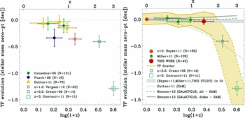
Figure 16. Evolution of the Tully–Fisher relationship zeropoint with redshift from Miller et al. (Reference Miller, Ellis, Sullivan, Bundy, Newman and Treu2012). Points show zeropoint and error bars show RMS scatter around the linear relations. The left panel shows mostly previous IFS results showing considerable disagreement. The right panel shows the results from Miller et al's very deep multi-slit work claiming no evolution in the zeropoint and very small scatter to z ~2. Some galaxy models and empirical fits are also shown (see Miller et al. for details). There is a clear inconsistency between the (shallower) IFS results for 0.2 < z < 2 where the redshift ranges overlap. Fast evolution at z > 2 could be possible, however deeper surveys are needed to also verify the z > 2 IFS results. The local relation is that of Reyes et al. (Reference Reyes, Mandelbaum, Gunn, Pizagno and Lackner2011) which is based on that of Pizagno et al. (Reference Pizagno2007). Credit: from Figure 7 of Miller et al. (Reference Miller, Ellis, Sullivan, Bundy, Newman and Treu2012), reproduced by permission of the AAS.
Finally, it is interesting to note that some authors have tried to compute baryonic masses for high-redshift galaxies by adding to the stellar masses an estimate of gas mass using the observed star-formation rate surface density and the Kennicutt–Schmidt relationship. There is some evidence that this works in the sense that there is usually better agreement between dynamical masses and baryonic masses than with stellar masses (Puech et al. Reference Puech, Hammer, Flores, Delgado-Serrano, Rodrigues and Yang2010; Vergani et al. Reference Vergani2012; Gnerucci et al. Reference Gnerucci2011b; Miller et al. Reference Miller, Bundy, Sullivan, Ellis and Treu2011). In the local Universe, the ‘baryonic Tully–Fisher relationship’ is found to give a better linear relation, compared to stellar masses, down to low masses where galaxies become much more gas rich (McGaugh et al. Reference McGaugh, Schombert, Bothun and de Blok2000; McGaugh Reference McGaugh2005). This has been investigated at high-redshifts; Puech et al. (Reference Puech, Hammer, Flores, Delgado-Serrano, Rodrigues and Yang2010) found no evolution in the offset of the baryonic relation at z ~0.6 where the stellar relation showed evolution and interpreted this as a conversion of gas in to stars from a fixed well over cosmic time. (Alternatively, one might suppose galaxies accrete gas and could move along the relation.) Similar lack of zeropoint evolution was found at z > 1 by Vergani et al. (Reference Vergani2012). Given the range of results for the stellar mass zeropoint evolution (Figure 16) and the uncertainty introduced by estimating gas masses from star-formation I would argue that it is premature to over-interpret the baryonic Tully–Fisher relationship evolution. The local relation uses direct HI masses; it may be another decade before HI is available in normal galaxies at z≳1, but it would be interesting in the near future to consider this with estimates of molecular gas masses from CO data.
The other kinematic scaling relation is the velocity-size one. Bouché et al. (Reference Bouché2007) found that local spirals and z ~2 star-forming SINS galaxies overlap substantially in this plane and there is little evidence for evolution with the exception of sub-mm galaxies which were very compact. Puech et al. (Reference Puech, Hammer, Lehnert and Flores2007) found similar results at z ~0.6. In both cases, the scatter was considerable and not as tight as the mass–velocity relation, a result that mirrors the local Universe. Puech et al. interpreted extra scatter as arising from their disturbed kinematic classes and it is also true that the SINS sizes were for all objects, not just well-modelled discs. MASSIV finds only ≃ − 0.1 dex in size–mass and size–velocity relation (i.e. smaller discs at z ≃ 1.2 compared today). Dutton et al. (Reference Dutton2011b) note that the lack of evolution in size–velocity relations may be inconsistent with the sign of the observed Tully–Fisher relationship evolution (including those derived within the same survey such as SINS). They also compare with data from DEEP2 and size–mass relations from photometric surveys and argue that there is a consistent picture of early discs being smaller, as theoretically expected, and discrepancies can be attributed to (i) different methods and conversions of size measurements, (ii) selection biases in IFS surveys, and (iii) possible differences in sizes between the young stellar populations probed by ionised gas compared to stellar mass.
5.4 The merger rate
One key question that IFS surveys set out to address was the prevalence of mergers at high-redshift. Certainly one might have supposed they were common given the irregular structures of high-redshift galaxies (e.g. Baugh et al. Reference Baugh, Cole and Frenk1996) and an IFS is the instrument of choice for objects with unknown a priori kinematic axes. Merger rates can be investigated by looking at galaxy image irregularities (Conselice et al. Reference Conselice, Bershady, Dickinson and Papovich2003, Reference Conselice, Rajgor and Myers2008; Bluck et al. Reference Bluck, Conselice, Buitrago, Grützbauch, Hoyos, Mortlock and Bauer2012), but as we have seen there are numerous examples of clumpy galaxies which are morphologically irregular but kinematically regular.
Before the advent of IFS surveys, the primary method of estimating the merger rate at high-redshift was via pair counts, starting with Zepf & Koo (Reference Zepf and Koo1989); Carlberg, Pritchet, & Infante (Reference Carlberg, Pritchet and Infante1994); Le Fèvre et al. (Reference Le Fèvre2000); Lin et al. (Reference Lin2004), and many papers since. By trying to estimate the fraction of galaxies that were ‘interacting pairs’ $f_{\text{int}}$
(e.g. close on the sky, using redshift and tidal feature information if available) and then adding a merger timescale
$f_{\text{int}}$
(e.g. close on the sky, using redshift and tidal feature information if available) and then adding a merger timescale $T_{\text{merge}}$
(usually calibrated via simulations), one can estimate a merger rate
R:
$T_{\text{merge}}$
(usually calibrated via simulations), one can estimate a merger rate
R:
 \begin{equation}
R = \frac{f_{\text{int}}}{T_{\text{merg}}}
\end{equation}
\begin{equation}
R = \frac{f_{\text{int}}}{T_{\text{merg}}}
\end{equation} $T_{\text{merg}}$
is set by dynamical friction and is around 1 Gyr (Lotz et al. Reference Lotz, Jonsson, Cox and Primack2008; Kitzbichler & White Reference Kitzbichler and White2008; Lotz et al. Reference Lotz, Jonsson, Cox, Croton, Primack, Somerville and Stewart2011), noting that not all pairs identified in surveys will eventually merge and this effect is often incorporated implicitly in to the calibration (the non-merging fraction may be around 30–50% for typical observational selections; Kitzbichler & White (Reference Kitzbichler and White2008)). The star-formation rates in close pairs may even be enhanced as far as 150 kpc (Patton et al. Reference Patton, Torrey, Ellison, Mendel and Scudder2013) which at this distance are not likely future mergers; but such effects do make clear the point that one should be careful of selection effects in pair catalogues especially in the rest-frame optical.
$T_{\text{merg}}$
is set by dynamical friction and is around 1 Gyr (Lotz et al. Reference Lotz, Jonsson, Cox and Primack2008; Kitzbichler & White Reference Kitzbichler and White2008; Lotz et al. Reference Lotz, Jonsson, Cox, Croton, Primack, Somerville and Stewart2011), noting that not all pairs identified in surveys will eventually merge and this effect is often incorporated implicitly in to the calibration (the non-merging fraction may be around 30–50% for typical observational selections; Kitzbichler & White (Reference Kitzbichler and White2008)). The star-formation rates in close pairs may even be enhanced as far as 150 kpc (Patton et al. Reference Patton, Torrey, Ellison, Mendel and Scudder2013) which at this distance are not likely future mergers; but such effects do make clear the point that one should be careful of selection effects in pair catalogues especially in the rest-frame optical.
In determining the galaxy merger rate from kinematics, one arrives at a similar equation:
 \begin{equation}
R = \frac{ f_{\text{merg}} }{T^{\prime }_{\text{merg}}}
\end{equation}
\begin{equation}
R = \frac{ f_{\text{merg}} }{T^{\prime }_{\text{merg}}}
\end{equation} $f_{\text{merge}}$
is the fraction of galaxies identified as mergers from kinematics, and
$f_{\text{merge}}$
is the fraction of galaxies identified as mergers from kinematics, and $T^{\prime }_{\text{merge}}$
is the timescale. Note this is a different timescale from Equation (20) as we are now considering closer galaxies and a more advanced merger stage. However, R should be the same (for an equivalent sample) as galaxies would be conserved at all phases of the merging process (Conselice, Yang, & Bluck Reference Conselice, Yang and Bluck2009). One expects both timescales to be of order 1 Gyr (Puech et al. Reference Puech, Hammer, Hopkins, Athanassoula, Flores, Rodrigues, Wang and Yang2012) but both can vary by factors of 2–3 (Lotz et al. Reference Lotz, Jonsson, Cox and Primack2008). Chou, Bridge, & Abraham (Reference Chou, Bridge and Abraham2012) found that only ~20% of close pairs at z < 1 were kinematically associated, that the merging timescale was rather short (<0.5 Gyr), and that merging was dominated by blue–blue pairs (i.e. opposed to red on red ‘dry mergers’).
$T^{\prime }_{\text{merge}}$
is the timescale. Note this is a different timescale from Equation (20) as we are now considering closer galaxies and a more advanced merger stage. However, R should be the same (for an equivalent sample) as galaxies would be conserved at all phases of the merging process (Conselice, Yang, & Bluck Reference Conselice, Yang and Bluck2009). One expects both timescales to be of order 1 Gyr (Puech et al. Reference Puech, Hammer, Hopkins, Athanassoula, Flores, Rodrigues, Wang and Yang2012) but both can vary by factors of 2–3 (Lotz et al. Reference Lotz, Jonsson, Cox and Primack2008). Chou, Bridge, & Abraham (Reference Chou, Bridge and Abraham2012) found that only ~20% of close pairs at z < 1 were kinematically associated, that the merging timescale was rather short (<0.5 Gyr), and that merging was dominated by blue–blue pairs (i.e. opposed to red on red ‘dry mergers’).
One approach to measuring merger rates more precisely is to take a close pair catalogue and confirm the kinematic association spectroscopically using slit spectroscopy (Chou et al. Reference Chou, Bridge and Abraham2012). An interesting hybrid approach was used by López-Sanjuan et al. (Reference López-Sanjuan2013), where they took advantage of the fact that their IFS maps were wider field than typical to count close kinematic pairs (within ~20 kpc and 500 km s−1) as well as advanced ongoing mergers for star-forming galaxies with 1010−10.5M⊙. Good agreement was found by López-Sanjuan et al. between their kinematic and other's photometric surveys at 1 < z < 1.5. Their ‘major merger fraction’ (meaning 1:4 at least ratios) was ~20% over this redshift interval translating to a merger rate of ~0.1 Gyr−1 (this is equivalent for a typical $T^{\prime }_{\text{merg}} \simeq 2$
Gyr which is what simulations typically indicate for pairs within 20 kpc, Kitzbichler & White Reference Kitzbichler and White2008). They found this to be consistent with lower redshift photometric studies with an overall evolution of (1 + z)4 in the rate. Extrapolation of their power-laws would predict close to a 100% merger fraction at z = 2.5 (and a rate of ~0.7 Gyr−1), which seems inconsistent with the results of the SINS (Förster Schreiber et al. Reference Förster Schreiber2009) and AMAZE-LSD surveys (Gnerucci et al. Reference Gnerucci2011b) which both observe kinematic fractions of closer to ~30%. One possibility is that these surveys may be missing close pairs which have not yet progressed to the kinematic stage, however the MASSIV data by itself suggests a constant rate at z > 1 so perhaps the power-law evolution could be flattening off at z > 1. A direct comparison of merger fractions and rates from purely photometric pairs would be valuable at 2 < z < 3. Bluck et al. (Reference Bluck, Conselice, Bouwens, Daddi, Dickinson, Papovich and Yan2009) looked at pairs (mass ratio 1:4) within 30 kpc of >1011M⊙ galaxies at 1.7 < z < 3, the inferred merger rate is ~1 Gyr−1 (their Figure 3) which seems consistent with the higher MASSIV extrapolation; however, the mass range is different and would include a substantial fraction of quiescent non-star-forming galaxies than does MASSIV and SINS. Slit surveys of z~3 LBGs seem to find a surprisingly high fraction of spectroscopic pairs (i.e. double lined) which could also imply a higher merger rate (Cooke et al. Reference Cooke, Berrier, Barton, Bullock and Wolfe2010). Such a high merger/interaction rate at z > 2 typically does not match modern ΛCDM model predictions, (Bertone & Conselice Reference Bertone and Conselice2009), (though see Cooke et al. for a contrary view).
$T^{\prime }_{\text{merg}} \simeq 2$
Gyr which is what simulations typically indicate for pairs within 20 kpc, Kitzbichler & White Reference Kitzbichler and White2008). They found this to be consistent with lower redshift photometric studies with an overall evolution of (1 + z)4 in the rate. Extrapolation of their power-laws would predict close to a 100% merger fraction at z = 2.5 (and a rate of ~0.7 Gyr−1), which seems inconsistent with the results of the SINS (Förster Schreiber et al. Reference Förster Schreiber2009) and AMAZE-LSD surveys (Gnerucci et al. Reference Gnerucci2011b) which both observe kinematic fractions of closer to ~30%. One possibility is that these surveys may be missing close pairs which have not yet progressed to the kinematic stage, however the MASSIV data by itself suggests a constant rate at z > 1 so perhaps the power-law evolution could be flattening off at z > 1. A direct comparison of merger fractions and rates from purely photometric pairs would be valuable at 2 < z < 3. Bluck et al. (Reference Bluck, Conselice, Bouwens, Daddi, Dickinson, Papovich and Yan2009) looked at pairs (mass ratio 1:4) within 30 kpc of >1011M⊙ galaxies at 1.7 < z < 3, the inferred merger rate is ~1 Gyr−1 (their Figure 3) which seems consistent with the higher MASSIV extrapolation; however, the mass range is different and would include a substantial fraction of quiescent non-star-forming galaxies than does MASSIV and SINS. Slit surveys of z~3 LBGs seem to find a surprisingly high fraction of spectroscopic pairs (i.e. double lined) which could also imply a higher merger rate (Cooke et al. Reference Cooke, Berrier, Barton, Bullock and Wolfe2010). Such a high merger/interaction rate at z > 2 typically does not match modern ΛCDM model predictions, (Bertone & Conselice Reference Bertone and Conselice2009), (though see Cooke et al. for a contrary view).
Another possible tension is at z ~0.6. The IMAGES survey find a high fraction of galaxies with anomalous IFS kinematics (Neichel et al. Reference Neichel2008; Yang et al. Reference Yang2008; Hammer et al. Reference Hammer, Flores, Puech, Yang, Athanassoula, Rodrigues and Delgado2009) which is interpreted as a high merger fraction, 33% involved in major mergers (Puech et al. Reference Puech, Hammer, Hopkins, Athanassoula, Flores, Rodrigues, Wang and Yang2012). The close pair studies mentioned above suggest the merger fraction is closer to 4% at z ~0.6 (e.g. see Figure 24 of López-Sanjuan et al. Reference López-Sanjuan2013) and if the timescales are similar then these should be comparable and clearly they are not. Puech et al. argued that a fraction of their objects were in what they called a ‘post-fusion’ phase, these should be compared to close pairs at an earlier epoch (z ~1.1) which lessens the tension due to the fast evolution in pairs with redshift.
However, the fact remains that if 33% of star-forming galaxies are deeply kinematically disturbed at only z ~0.6 and one must ask the question how is this compatible with the fact that the majority of star-forming large galaxies today have thin, fragile discs. The traditional view is that a major merger quenches star-formation in a galaxy and forms a red-sequence elliptical; the morphological transformation is one way and its star-forming life is then over. However, in CDM models it has long been supposed that such ellipticals could continue to accrete gas (either pristine or expelled during the merger) and form new discs of young stars; they would then transform back in to a spiral albeit one with a large bulge-to-disc ratio (Barnes Reference Barnes2002; Springel & Hernquist Reference Springel and Hernquist2005). Hammer et al. (Reference Hammer, Flores, Puech, Yang, Athanassoula, Rodrigues and Delgado2009) posit a ‘sprial rebuilding scenario’ in which half of today's major spirals were in an active major merger phase 6 Gyr ago, and all have had a merger since z = 1, (with the Milky Way being exceptional) and the disc is then rebuilt by re-accreting the original gas. This may have more angular momentum than cosmological accretion as it retains that of the original disc. Puech et al. suggested that the high star-formation rate of discs at z ~0.6 would permit them to regrow rapidly. Such a large recent merger rate is contingent on the results from the IMAGES survey being correct; it is possible they have overestimated the fraction of galaxies with anomalous kinematics—deeper slit surveys have found a considerably smaller fraction of kinematically irregular galaxies at this epoch (Miller et al. Reference Miller, Bundy, Sullivan, Ellis and Treu2011). As well as being a shallower depth, the IMAGES data had a very coarse sampling of their kinematic maps making interpretation difficult (see Section 3.3).
The main caveats in these comparisons of IFS-derived merger rates with other techniques (and indeed in general with inter-techniques comparisons) are the fact that (i) different surveys are probing different mass ranges, different galaxy populations with different selections even if they are at the same redshift and (ii) the time scales for the different stages of the merger process are a key model uncertainty in converting observed fractions in to rates. One final comment on this: comparing the form Equations (20) and (21), I note that it is immediately obvious that if one wishes to establish the consistency of photometric and kinematic merger rates, one only needs to know the ratio of timescales $T_{\text{merg}} / T^{\prime }_{\text{merg}}$
of the different phases. This ratio may have a large range (ratio of 2–12, Conselice et al. Reference Conselice, Yang and Bluck2009) depending on the orbital parameters and is complicated by non-merging pairs. While the absolute values may be poorly constrained from simulations, it is interesting to speculate if the ratio might be better constrained, for example does it vary strongly with mass ratio? The application of simulations to investigate this further would be interesting future work.
$T_{\text{merg}} / T^{\prime }_{\text{merg}}$
of the different phases. This ratio may have a large range (ratio of 2–12, Conselice et al. Reference Conselice, Yang and Bluck2009) depending on the orbital parameters and is complicated by non-merging pairs. While the absolute values may be poorly constrained from simulations, it is interesting to speculate if the ratio might be better constrained, for example does it vary strongly with mass ratio? The application of simulations to investigate this further would be interesting future work.
6 OUTSTANDING QUESTIONS AND FUTURE DIRECTIONS
One thing that has become outstandingly clear in the course of this review is that we have only obtained cursory answers to the questions that IFS surveys have set out to investigate. Certainly, we can see some definite discs and mergers at high-redshift and make plausible physical models; however, the detailed abundance of these kinematics classes remains uncertain. The IFS surveys have been pioneering, however like all pioneers they have set off in different directions, explored limited areas and different terrain. When they compare notes they find they all have done things somewhat differently, they all agree on some of the major landmarks but the systematic detail is subject to a lot of difficult inter-comparisons.
6.1 Outstanding questions
The outstanding questions remaining follow the themes of the section of this review. I will highlight some of the most important in my mind:
Discs at high-redshift? As I have discussed clearly many of the objects observed at high-redshift in IFS surveys are rotating with velocity fields that rise and turnover to a flat portion in a manner similar to local discs. It is not at all clear what fraction are discs at what redshift, the range is 30–100% of star-forming galaxies and different surveys probe to different depths, sample different redshifts, and select different mass ranges. It is clear though that pure consideration of imaging surveys is not enough to establish the epoch at which discs arise in the Universe, as is often still done (e.g. Mortlock et al. Reference Mortlock2013). The scatter in the Tully–Fisher relationship may be increasing at high-redshift, or it may not. Deeper IFS surveys are needed to probe the turnover in galaxy rotation curves at z > 1. We also need greater overlap between broad-band HST surveys and kinematic AO surveys (only a few papers each with only a few objects). Some objects may be too small to resolve as discs in natural seeing, and some may even be too small (<1 kpc) to resolve with AO data. The discs are certainly morphologically different to local ones: at a minimum they have much higher star-formation rates, have a high-velocity dispersion, and are physically thick. I note Law et al. (Reference Law, Steidel, Shapley, Nagy, Reddy and Erb2012b) found they may be even more different: axial ratios provide some evidence that some may be triaxial ellipsoidal systems. Similar results have been found by Chevance et al. (Reference Chevance, Weijmans, Damjanov, Abraham, Simard, van den Bergh, Caris and Glazebrook2012) for compact red galaxies. Nor is it clear whether the discs we see at high redshift are evolving in to the thick discs of today's spirals, or S0 galaxies, or massive ellipticals (via major mergers). These questions could perhaps be tested in the future by considering space density (van Dokkum et al. 2010) and clustering (Adelberger et al. Reference Adelberger, Erb, Steidel, Reddy, Pettini and Shapley2005) of such objects as a means of tracing from high to low-redshift. Parent populations have been studied (Hayashi et al. Reference Hayashi, Shimasaku, Motohara, Yoshida, Okamura and Kashikawa2007; Lin et al. Reference Lin2012) but current IFS sub-samples are not well-characterised in a mass-complete sense.
What are ‘dispersion-dominated galaxies’? The existence of star-forming non-rotating galaxies is hard to explain. They start to appear at masses >1010M⊙ for z > 1. High star-formation implies large amounts of gas which naturally settles in to a disc on dynamical time. Unresolved (even at AO resolution) very compact discs would be one possibility as argued by Newman et al. (Reference Newman2013). Law et al. (Reference Law, Steidel, Shapley, Nagy, Reddy and Erb2012b) found that the morphology is not truly disc-like and suggested that may in fact indeed be transient structures, not in equilibrium, perhaps merger driven. If transient events are common and enhance star-formation, they may naturally populate UV-selected samples. More detailed comparisons of the morphological axial ratios vs. stellar mass and specific star-formation rate would be interesting especially given the wealth of new near-IR structural data coming from HST in the CANDELS survey (Grogin et al. Reference Grogin2011; Koekemoer et al. Reference Koekemoer2011). The final answer to the question of the structure of these compact galaxies may depend on 30-m class telescope AO resolution, though it is possible that the sub-resolution kinematics could be tested with spectroastrometry.
The nature and driver of dispersion? The large resolved velocity dispersion of high-redshift galaxies was an unexpected observation. It is intrinsic and is not a beam-smearing effect. What is measured is the ionised gas dispersion as revealed by emission lines. One naturally then asks is it coming from HII regions bound to a disc, in which case it reflects the gas disc dispersion, or from outflowing ionised gas? The consensus seems to be the former, and in fact outflows are seen to be separately observed in even broader line wings of width 300–1 000 km s−1 (Genzel et al. Reference Genzel2011; Wisnioski et al. Reference Wisnioski, Glazebrook, Blake, Poole, Green, Wyder and Martin2012). A key test of this was measuring the dispersion of the cold molecular gas (Tacconi et al. Reference Tacconi2010, Reference Tacconi2013; Swinbank et al. Reference Swinbank2011; Hodge et al. Reference Hodge, Carilli, Walter, de Blok, Riechers, Daddi and Lentati2012), this will be improved to sub-galactic scales by the resolution and sensitivity of new telescopes such as ALMA. The resolved stellar kinematics of the young disc also ought to match the gas, however this has to be measured from absorption lines which will likely require 30 m class telescopes. If we interpret the dispersion as a turbulent gas disc then the energy source powering it is not known. The picture of Q = 1 marginally stable discs requires but does not specify this. Cosmic accretion, star-formation feedback, clump formation, and stirring are all interesting candidates and progress will require a difficult quantitative estimate of these across large samples. Structure seems apparent in numerous dispersion maps of galaxies (see discussion in Section 5.1) but is never commented on. Is it real and if so what does is correlate with? This may provide additional physical insight.
The physics of clumps? We have seen a picture of the large clumps seen in high-redshift galaxies as Jeans mass objects embedded in galaxy discs. This explains the important observation of irregular morphology but smooth velocity fields without significant perturbations at the clump locations. Their masses, luminosities, sizes and velocity dispersion seem to scale with star-formation rates, however it is not clear if there are single scaling relations connecting them with galactic HII regions today or two sequences. Part of this is that size measurements are particularly difficult to define even locally, HII regions clump together in complexes in spiral arms and the apparent size depends on the spatial resolution and image depth (Rozas et al. Reference Rozas, Beckman and Knapen1996). More uniform and systematic approaches to comparing local and high-redshift galaxies (including quantitative artificial redshifting) are needed.
We do know that the clumps we see in high-redshift galaxies are not just a resolution effect, i.e. the morphology is fundamentally different from artificially redshifted local galaxies (Elmegreen et al. Reference Elmegreen, Elmegreen, Marcus, Shahinyan, Yau and Petersen2009b), however we do not know if these clumps will break up in to sub-clumps when viewed at even higher angular resolution. If they do, then which clump scale is important for scaling relations? Are the clumps (or sub-clumps) single bound structures with the velocity dispersion providing virial support? Do they also have rotational support (Ceverino et al. Reference Ceverino, Dekel and Bournaud2010)? How does metallicity, ionisation, stellar population age, and dust extinction compare for young clumps vs. the surrounding disc and radius within a galaxy? These could all be uncovered by future IFS observations. One would presume that clumps also contain large amounts of cold molecular gas fuelling the star-formation. Do they contain super-Giant Molecular Clouds and what are their structure? One particularly clear and notable example of molecular clumps has been seen at z = 4.05 in a sub-mm galaxy (albeit one of the most luminous) by Hodge et al. (Reference Hodge, Carilli, Walter, de Blok, Riechers, Daddi and Lentati2012). Future observations from ALMA and other facilities will produce many more such observations of the general galaxy population extending to lower redshift. They are likely to test the picture that clumps form in regions of Q < 1 by measuring Q properly using direct gas surface density measurements. Finally, one must ask what is the fate of giant clumps, do they last a long time and gradually spiral in to the centre of a galaxy and form a bulge or are they quickly destroyed by intense feedback? Simulations support both short (Genel et al. Reference Genel2012) and long lifetime (Ceverino et al. Reference Ceverino, Dekel, Mandelker, Bournaud, Burkert, Genzel and Primack2012) scenarios depending on assumptions, observations (Genzel et al. Reference Genzel2011; Wuyts et al. Reference Wuyts2012; Guo et al. Reference Guo, Giavalisco, Ferguson, Cassata and Koekemoer2012) have yet to settle the question.
The Star-Formation Law? We have seen that stars form in high-redshift galaxies in very different conditions than they do locally. The discs are more gas rich implying much greater pressure, the star-formation feedback is more intense especially within clumps and the dispersion of the disc is much greater. Given the star-formation history of the Universe (Hopkins & Beacom Reference Hopkins and Beacom2006), most stars formed under these conditions. One must therefore ask basic questions, for example is the star-formation law the same? Does a Kennicutt–Schmidt-like law apply or something different? The classical Kennicutt–Schmidt relationship simply relates projected surface densities of gas and star-formation via a power law. The thickness of high-redshift discs would imply quite different results from laws that depend on projected surface densities vs. volumetric densities (Krumholz, Dekel, & McKee Reference Krumholz, Dekel and McKee2012). There are many other proposed variations on this theme. For example, there may be ‘thresholds’ to star-formation (e.g. above some critical density, Lada, Lombardi, & Alves Reference Lada, Lombardi and Alves2010; Heiderman et al. Reference Heiderman, Evans, Allen, Huard and Heyer2010). At high-redshift, it has been suggested that there are in fact two relations—a ‘sequence of starbursts’ and a ‘sequence of discs’ but which may be unified by introducing a dynamical time in to the formulation (Daddi et al. Reference Daddi2010b). Alternatively, it may simply reflect issues with CO conversion factors (Kennicutt & Evans Reference Kennicutt and Evans2012). Direct resolved tests of star-formation laws in high-redshift galaxies (see Freundlich et al. Reference Freundlich2013 for a first step towards this) are critical and will improve with the advent of high-resolution ALMA data in the next few years. Another related topic is the Initial Mass Function (IMF) for star-formation. The possibility of IMF variations is important (see review of Bastian, Covey, & Meyer Reference Bastian, Covey and Meyer2010) and evidence for variations in galaxies has attracted considerable recent interest and some tantalising results (e.g. Hoversten & Glazebrook Reference Hoversten and Glazebrook2008; Meurer et al. Reference Meurer2009; van Dokkum & Conroy Reference van Dokkum and Conroy2010; Cappellari et al. Reference Cappellari2012). It seems plausible that the IMF could be different in high-redshift discs and/or in clumps (e.g. Narayanan & Davé Reference Narayanan and Davé2012) and perhaps could be investigated by comparing colours and spectra as are done at low-redshift.
The merger rate? As we have seen there seems to be some tension between some IFS results and those of other techniques. In particular, at z ~0.5 deeper and higher resolution IFS observations are needed to determine if nearly half of all star-forming galaxies have major kinematic disturbances or whether this is just an artefact of low angular resolution or not being sensitive to galaxy outskirts. There is a clear tension with the estimates of the merger rate by close pairs, and at these redshifts this technique is quite sensitive. At high-redshift (z > 2) some estimates for Lyman Break Galaxies put the merger fraction close to 100%, this may be compatible with the existence of massive discs and the lower rates found in IFS surveys as the UV-selected objects are at the lower mass end. Can we define a consistent merger rate across the various merger phases from close approach through to coalescence as a function of stellar mass, merger ratio, and redshift? This would be a powerful constraint on galaxy formation models. Deeper and more numerous IFS observations will help, but in my opinion it is equally important to find new techniques to extract time scales and mass ratios from IFS maps (which would obviously have to be calibrated on simulations).
In a sense, every galaxy at high-redshift is being subject to a continual accretion of matter of some degree of lumpiness, it is a question of degree and how often. Every disc at high-redshift has probably had some sort of kinematic disturbance in its recent past, likewise every major merger remnant is probably busily regrowing a disc from new infall. Being able to quantify these effects continuously would be more helpful in comparison with models than the current somewhat artificial distinction between ‘disc’ and ‘merger’ which is predicated on the modern Universe where mergers are infrequent.
6.2 New surveys
Clearly, one next and critical step at high-redshift is large-scale IFS surveys of thousands of objects with uniform, homogeneous selection functions. Current surveys suffer from diversity—selection is done using UV flux, near-IR flux, sub-mm flux, emission line flux, or some difficult to evaluate combination of all these. Even then selection from the parent sample is not necessarily homogeneous. Of course the limiting factor in survey size to date has been the necessity to observe one object at a time with IFS (with the notable exception of the IMAGES survey using the optical FLAMES-GIRAFFE instrument). The instrument that is most likely to transform this is KMOS, recently commissioned at the end of 2012, on the VLT (Sharples et al. Reference Sharples2012) which will work in the near-infrared and offer a 24-IFU multiplex (in natural seeing). Multiplexed observations facilitate an improvement in numbers of course, but they also permit an improvement in depth as well as the telescope time is less expensive per object. A number of groups are proposing IFS surveys of this scale with KMOS. It remains desirable to select galaxies for IFS from spectroscopic redshift surveys with prior information of the strength of the emission lines and their proximity to night sky lines. New redshift surveys using slitless spectroscopy in space will allow this (Brammer et al. Reference Brammer2012); as will new near-IR redshift surveys using new multi-slit instruments such as MOSFIRE on Keck (McLean et al. Reference McLean2012). They will also provide well-defined environments for the IFS kinematic observations at high-redshift; a topic that so far has been completely unaddressed. If turbulent discs are fuelled by ongoing cosmic accretion, one might speculate on seeing strong environmental trends in their incidence and star-formation rates.
With this prospect, I also think it is critical to see a move to a uniformity of application of kinematic techniques; a good example is disc fitting where every group has developed their own bespoke code. Large surveys need to develop a best practice with common codes and whole papers need to be devoted to describing and evaluating codes with full treatments of errors, fit qualities, and degeneracies. This is the same transformation as the photometric redshift community has gone through in the last decade as deep high-redshift imaging surveys have become industrialised.
Another analogy is with the first deep imaging and spectroscopic surveys done with CCDs in the 1980s and 1990s, it was immediately apparent that the local comparison surveys done with photography were inadequate and this spawned the Sloan Digital Sky Survey (York et al. Reference York2000). We seem to be in a similar position today with IFS surveys, they have been fruitful at handling objects with the complex morphological structures common at high-redshift, however the majority of the local comparison to date is with traditional work done with long-slit spectroscopy. This is changing rapidly as hundreds of local galaxies have been observed with wide field IFS instruments, notably the CALIFA (Sánchez et al. Reference Sánchez2012), ATLAS3D (Cappellari et al. Reference Cappellari2011a), and DISKMASS surveys (Bershady et al. Reference Bershady, Verheijen, Swaters, Andersen, Westfall and Martinsson2010). Low-redshift surveys are beginning with multi-IFU instruments; the MANGA survey in the US and the SAMI survey in Australia (Croom et al. Reference Croom2012) will both observe several thousand galaxies in the next few years with well-defined selection and environments. They will provide a ‘kinematic SDSS’ and allow the statistical comparison of rotation, velocity dispersion, and angular momentum vs. galaxy properties across a range of environments from the field to rich clusters allowing fundamental tests of galaxy formation models. I predict we will always move from simple scaling relations such as some measure of mass vs. rotation towards distribution functions, for example the space density vs. mass and angular momentum compared to theoretical models. These local surveys will also be extremely important for comparison with high-redshift; in particular the application of uniform techniques and the provision of large samples for artificial redshifting tests. This well-defined approach is necessary to settle the question of the evolution in the Tully–Fisher relationship — for example it is critical to test for selection biases to uncover the small amounts of evolution if any. Particularly important is these will provide high-quality baseline samples of galaxy mergers where kinematic features as well as low surface brightness photometric features (such as tidal tails) are available, confirming the merger nature but also providing approximate mass ratio estimates by comparison with simulations. We will also likely see an increasing number of other rare objects discovered that are similar to high-redshift galaxies (see Section 3.9) and whose close proximity will facilitate detailed astrophysical observation, in particular multi-wavelength observations to measure gas content and its role in shaping galaxy kinematics.
Future AO surveys will also be critical. It has been surprising how much progress has been made using natural seeing surveys given how under-sampled the galaxies are. AO surveys can deliver the kpc resolution required to resolve detailed internal structure and to make fundamental kinematic classifications of compact galaxies. Detailed study of individual galaxies will remain an important complement to the large surveys of thousands of galaxies with lower resolution. The main difficulty is that AO surveys remain small and it is difficult to see how substantial progress will be made in increasing sample size in the near-future given AO systems generally correct a small field-of view, hence no multiplexing of targets. Another difficulty of the current situation is the lack of significant samples which have had AO and non-AO observations of the same galaxies for comparison. Even groups who have done AO and non-AO observations have not done so for the same objects (a notable exception being Newman et al. (Reference Newman2013) however only limited comparisons have so far been made). Part of the reason for the limited size of AO overlap samples is the requirement for bright guide stars—even with laser guide star AO it is currently necessary to have a R ≲ 17 mag tip-tilt correction star and this has severely limited sample selection to only 10–20% of possible targets. The other issue is of course sensitivity—at higher spatial resolution one has less photons per spaxel but also light is lost in the AO optical system and through the imperfect correction (i.e Strehl ratios well less than unity). Thus, more compact sources or those with highly clumped high surface-brightness emission tend to be favoured and AO surveys have only had moderate completeness rates except when very long integration times have been attempted. Yet another restriction is the redshift coverage—strong emission lines need to be used and AO works best at the redder near-IR wavelengths. We are currently subject to an ‘AO redshift desert’ at 0.3 < z < 1.2 where we can not attain kpc resolution. The reddest strong emission line is Hα which only achieves good Strehl in the H-band for z > 1.2. The next reddest strong star-formation line is Pa α but that redshifts in to the thermal infrared for z > 0.3.
Many of these issues are gradually being improved. Next generation AO systems will deliver higher throughput and higher Strehl at shorter wavelengths enabling AO observations of z < 1 galaxies. Signal:noise is also improved by new near-IR detectors with lower readout noise (which is an issue due to the high spectral resolution of kinematic observations). Guide star availability is being improved through more efficient wavefront sensors, near-IR wavefront sensors, which helps because so many faint stars are red M-stars, (Max et al. Reference Max, McGrath, Gavel, Le Mignant, Wizinowich and Dekany2008), the development of compromise ‘no tip tilt’ laser AO modes (Davies et al. Reference Davies2008), and the development of ‘Adaptive Optics Deep Fields’ with low galactic extinction and high stellar density (Damjanov et al. Reference Damjanov2011). Multiple object integral field AO observations (denoted ‘MOAO’) may also become possible due to the development of compact deployable wavefront sensors (Andersen et al. Reference Andersen2006b) allowing greater number of objects and longer integration times. AO work will extend down in to the optical as technology improves, for example the next generation MUSE instrument on VLT (Arsenault et al. Reference Arsenault2008) will offer a diffraction-limited visible imaging mode with a 7.5 arcsec IFU (as well as a contiguous 1 arcmin wide field mode). Finally, the advent of 20–40 m class telescopes in the 2020s will increase both AO resolution (from the diffraction limit) and light gathering power. Ultimately in my view large and complete AO IFS surveys will have greater impact on our physical understanding, but will take longer to arrive, than large seeing-limited surveys.
Even AO surveys can be under-sampled when some galaxy sizes approach a kpc at high-redshift (van Dokkum et al. Reference van Dokkum2008; Damjanov et al. Reference Damjanov2009; Wuyts et al. Reference Wuyts2011). The future prospects are also very bright for taking advantage of the extra spatial resolution boost from gravitational strong-lensing which coupled with AO and allowed us to probe sub-kpc scales (Stark et al. Reference Stark, Swinbank, Ellis, Dye, Smail and Richard2008; Jones et al. Reference Jones, Swinbank, Ellis, Richard and Stark2010; Livermore et al. Reference Livermore2012). New sky surveys such as the Dark Energy Survey (Flaugher Reference Flaugher2005), the Hyper Suprime-Cam survey (Takada Reference Takada2010), and the Large Synoptic Sky Telescope (Tyson Reference Tyson2002) survey will produce thousands to tens of thousands of new strong-lens candidates allowing a greater diversity of objects to be studied and statistics to be assembled. As such targets only have a sky density of order one per deg2 they do not suffer a relative disadvantage from the single-object nature of AO and there ought to be ample with suitable tip-tilt stars.
I predict the most important developments in the immediate future (the next five years) will not be at optical wavelengths. The Atacama Large Millimeter/sub-millimeter Array (ALMA) (Hills & Beasley Reference Hills and Beasley2008) is being commissioned in Chile and is being officially inaugurated this year and is likely to dominate the near-future of high-redshift galaxy kinematics. Why do I make this statement? Today, high-redshift is dominated by optical and near-IR observations which are mainly sensitive to stars and hot ionised gas (e.g. from star-formation or AGN). However, it is important to consider ‘the fuel as well as the fire’. We have seen from existing sub-mm observations that high-redshift galaxies are rich in molecular gas (Daddi et al. Reference Daddi2010b; Tacconi et al. Reference Tacconi2010). Current sub-mm telescopes barely resolve high-redshift galaxies with their beams of 0.5–1 arcsec and require many hours of integration per galaxy. However, integration time performance of radio telescopes scales much faster with increased area (∝A 2) than do background-limited optical telescopes (∝A 1/2). ALMA will have three times more collecting area and baselines up to 16 km and hence will improve resolution and integration times by factors of ten. In the northern hemisphere, upgrades to the Plateau de Bure Interferometer (the ‘NOEMA’ project) will double the number of dishes (increasing the collecting area to 40% of full ALMA) and maximum baselines (allowing sub-arcsec resolution) by 2018. Upgrades to lower frequency radio interferometers may enable such studies to be extended to even higher redshifts. These new facilities will enable kpc-resolution morphology and kinematics of molecular gas and dust in normal star-forming galaxies to be routinely made. The ‘turbulent clumpy disc model’ predicts galaxies to be gas rich and thick. Will we see thick cold molecular gas discs co-rotating and aligned with the young stars seen by the near-IR IFS observations? Will we see super-giant molecular clouds associated with the bright giant star-forming regions seen in the UV? I predict we will! It should be noted though that the observations are likely to be even more time-consuming than optical/near-IR. Even with the full ALMA of 50 dishes I calculate that 0.3 arcsec/50 km s−1 resolution CO(3-2) observations of a z = 2.0 galaxy with 1011M⊙ of molecular hydrogen would take 20 h.Footnote 22 On the other hand, the ~one arcmin field-of-view and wide bandwidth of ALMA could allow multiple targets at similar redshifts to be observed simultaneously, somewhat offsetting this.
Another extremely important question for these high-resolution sub-mm facilities is the nature of the star-formation law relating gas density to star-formation rate, a critical theoretical ingredient of numerical galaxy formation simulations (this is often referred to as the ‘sub-grid physics’). Around 80% of the stars in the Universe formed at z > 1 but we have seen throughout this review that galaxies in the high-redshift Universe are physically very different from today's galaxies. Will the star-formation law be the same as in today's galaxies or quite different? Future facilities will bring a highly superior set of data to bear on this important problem and I will predict some surprises! Finally one interesting new prediction that could perhaps be tested by ALMA is the possible existence of dark turbulent discs (Elmegreen & Burkert Reference Elmegreen and Burkert2010). The prediction is that turbulence in gas discs starts initially in a dark accretion-driven phase lasting for ~180 Myr before star-formation turns on and renders the galaxy optically visible. The gas would be cold and molecular—the actual visibility of such objects to ALMA has not yet been calculated, but would make for an interesting paper.
6.3 Final words
I am fortunate in the timing of this review as I sense that in 2013 we are now at the end of the first major phase of high-redshift IFS kinematic studies which started around 2005. My impression of the topic is that in the next few years, we are going to see a phase change in the field and an avalanche of new data from large surveys with instruments such as KMOS and the first sub-mm wavelength kinematic studies at high angular resolution. Large surveys with consistent selection will allow us to firmly address the statistical questions about the incidence of kinematic structures that have been identified at high-redshift and longer wavelength observations will allow us to view the cold molecular gas, both before and after forming stars, directly. The combination of improved AO instruments and sub-mm telescopes will allow us to test the detailed physics of internal star-formation and probe galactic structure at high-redshift. I will look forward to seeing some of the outstanding physical questions raised by the first generation of surveys answered.
ACKNOWLEDGEMENTS
I would like to thank Bridget Glazebrook for her love and support in the long weekends required to write this review and the various little Glazebrooks for not creating too much disruption. I would also like to thank Bryan Gaensler for inviting me to write the very first Dawes review and continual reminders about my progress! Special thanks for providing useful references along the way go to Jeff Cooke, Andy Green, Luc Simard, and Emily Wisnioski. I would like to thank Roberto Abraham for a careful and critical review of the draft manuscript. Thanks also go to Reinhard Genzel, Richard Ellis, Sarah Miller, Susan Kassin, Joss Hawthorn, Karín Menéndez-Delmestre, Enrica Bellocchi, Tucker Jones, and Francois Hammer for providing useful comments and suggestions on the submitted manuscript and I have tried to reflect most of them to the best of my ability. The final responsibility and/or blame for the content and opinions of this review remain with me alone. Finally, I would like to extend great thanks to the referee, Natascha Förster Schreiber, for many useful comments and suggestions which have greatly added to this review.


 Open access