


1. Introduction
Galaxy clusters are megaparsec-sized systems that contain hundreds of individual galaxies which reside within a hot pool of ionised, magnetised gas. While some resident galaxies are typically observed to emit radio emission from their active galactic nuclei (AGN), very extended and diffuse radio sources originating from the intracluster medium (ICM) have been identified in a growing number of galaxy clusters over the last several decades (see van Weeren et al. Reference van Weeren2019, for a recent review). Theoretical and observational evidence support the suggestion that diffuse radio sources associated with the ICM are generated from the collisions, or mergers, of multiple galaxy clusters (e.g. Buote Reference Buote2001; Cassano et al. Reference Cassano, Ettori, Giacintucci, Brunetti, Markevitch, Venturi and Gitti2010). As dictated by the evolution of large-scale structure in the Universe, a cluster–cluster merger occurs on a timescale of about 1 Gyr (Sarazin Reference Sarazin2002), and during this time shock waves and turbulence are magnetically driven throughout the system. Turbulence and shocks can excite—and re-excite—relativistic electrons within the cluster magnetic field, leading to observable synchrotron emission at radio frequencies (e.g. Brunetti & Jones Reference Brunetti and Jones2014; Brunetti et al. Reference Brunetti2008; Brüggen et al. Reference Brüggen, Bykov, Ryu and Röttgering2012; Brüggen & Vazza Reference Brüggen and Vazza2015).
Merger-induced synchrotron sources can come in various forms (see Kempner et al. Reference Kempner, Blanton, Clarke and Soker2004, for a taxonomy). Some merging clusters host diffuse emission, known as giant radio halos, which fill the inner volume of the ICM. Other clusters show large, elongated structures on the outer edges of the ICM, called gischt-type radio relics or radio shocks. There are also cases where extended emission from resident radio galaxies is observed to be shock compressed or re-energised by a merger event of the host cluster. This type of emission does not always fit into a specific classification, but examples include the radio phoenixes in A13, A85, A133, and A4038 (Slee et al. Reference Slee, Roy, Murgia, Andernach and Ehle2001), the gently re-energised tail (GReET) in Abell 1033 (de Gasperin et al. Reference de Gasperin2017), the re-brightened tail in Abell 1132 (Wilber et al. Reference Wilber2018a), and the revived fossil plasma source found in Abell 1314 (Wilber et al. Reference Wilber2019, van Weeren et al., in preparation).
Radio halos are widely considered to be the result of turbulent re-acceleration of mildly relativistic electrons in the ICM (e.g. Brunetti et al. Reference Brunetti, Setti, Feretti and Giovannini2001; Donnert et al. Reference Donnert, Dolag, Brunetti and Cassano2013; Pinzke, Oh, & Pfrommer Reference Pinzke, Oh and Pfrommer2017). However, theory indicates that there should also be a population of secondary radio-emitting CRe produced from collisions between thermal protons and cosmic-ray protons in the ICM (hadronic model; Dennison Reference Dennison1980). It is still unknown as to how much of a role these secondary CRe play in generating radio halos since the expected gamma-ray contribution from these proton–proton collisions has yet to be detected in a single galaxy cluster (e.g. Ackermann et al. Reference Ackermann2010, Reference Ackermann2014; Prokhorov & Churazov Reference Prokhorov and Churazov2014).
Gischt-type relics, or radio shocks, are often found to trace bow shocks occurring on the largest scales and are therefore thought to be connected to diffusive shock acceleration that operates at a shock front (Blandford & Ostriker Reference Blandford and Ostriker1978; Ensslin et al. Reference Ensslin, Biermann, Klein and Kohle1998). X-ray observations of merging clusters typically show an overall disturbed morphology in their thermal gas; however, shock-heated gas can be identified by a sharp discontinuity in surface brightness (SB) and a corresponding jump from higher temperature to lower temperature for post-shock and pre-shock regions, respectively. To add to the challenge of their interpretation, not all merging clusters show evidence of shocks and not all detected shocks in merging clusters have radio counterparts (e.g. Botteon, Gastaldello, & Brunetti Reference Botteon, Gastaldello and Brunetti2018; Wilber et al. Reference Wilber2018b).
The details of the necessary acceleration mechanisms and the efficiencies of low Mach number shocks are still under scientific scrutiny (see Botteon et al. Reference Botteon, Brunetti, Ryu and Roh2020, for a recent study). Fermi-II acceleration prompted by merger turbulence and Fermi-I acceleration prompted by merger shocks are both usually too weak to accelerate electrons from thermal to ultra-relativistic energies (Botteon et al. Reference Botteon, Gastaldello, Brunetti and Dallacasa2016; Eckert et al. Reference Eckert2016; Kang, Ryu, & Jones Reference Kang, Ryu and Jones2012; Markevitch et al. Reference Markevitch, Govoni, Brunetti and Jerius2005; Petrosian & East Reference Petrosian and East2008; van Weeren et al. Reference van Weeren2016b). Hence, some form of pre-acceleration or a population of relativistic seed electrons is required to explain cluster-scale halos and relics. While primordial accretion shocks are suspected to account for a portion of the CRe population in clusters, AGN are another viable source for seed electrons. Several examples have been found where extended radio galaxies appear to be feeding into diffuse cluster sources: for example, the remnant radio galaxy supplying seeds for the relic in the Bullet cluster 1E 0657-55.8 (Shimwell et al. Reference Shimwell2015), the connection between a head-tail radio galaxy and relic in Abell 3411-3412 (Johnston-Hollitt Reference Johnston-Hollitt2017; van Weeren et al. Reference van Weeren2017), and the connection between the giant radio galaxy and the ultra-steep halo in Abell 1132 (Wilber et al. Reference Wilber2018a).
The origins of cluster magnetic fields are predicted to come from a constant primordial field that has been amplified over time (see Donnert et al. Reference Donnert, Vazza and Brüggen2018; Grasso & Rubinstein Reference Grasso and Rubinstein2001, for reviews). Recent investigations of the evolution of magnetic fields in merging galaxy clusters—through high-resolution cosmological magnetohydrodynamical simulations—have revealed that although major mergers can shift the peak magnetic spectra to small scales (via small-scale dynamo) in about 1 Gyr, continuous minor mergers are necessary for steady magnetic field growth over several Gyrs (Domínguez-Fernández et al. Reference Domínguez-Fernández, Vazza, Brüggen and Brunetti2019). Using the cryogenic X-ray microcalorimeter, soft X-ray spectrometer (Kelley et al. Reference Kelley2016), the Hitomi Collaboration et al. (2016) measured turbulent velocities in the Perseus cluster and found that the ICM was fairly quiescent, contradicting expectations. Synthesised observations (e.g. Roncarelli et al. Reference Roncarelli2018) of the not-yet-launched Athena X-ray satellite show that the X-ray Integral Field Unit spectrometer will have both unprecedented spectral resolution (2.5 eV at 7 keV) and spatial resolution ( ${\sim}$
few kpc) in measuring turbulence, even out to the cluster outskirts (see Simionescu et al. Reference Simionescu2019, for a recent review).
${\sim}$
few kpc) in measuring turbulence, even out to the cluster outskirts (see Simionescu et al. Reference Simionescu2019, for a recent review).
An ongoing project for the galaxy cluster science community is to gather sufficient data on a large number of ICM sources to allow for more thorough statistical studies of clusters. The Giant Metrewave Radio Telescope (GMRT) radio halo survey (Venturi et al. Reference Venturi, Giacintucci, Dallacasa, Cassano, Brunetti, Bardelli and Setti2008) and extended GMRT radio halo survey (Kale et al. Reference Kale2013) started this pursuit, providing observations of more than 60 galaxy clusters and finding radio halos in about  ${\sim} 23 \%$
of clusters. The LOFAR Two Metre Sky Survey (LoTSS; Shimwell et al. Reference Shimwell2017) is currently in progress to cover the entire northern hemisphere with very high sensitivity (
${\sim} 23 \%$
of clusters. The LOFAR Two Metre Sky Survey (LoTSS; Shimwell et al. Reference Shimwell2017) is currently in progress to cover the entire northern hemisphere with very high sensitivity ( $100\,\mu$
Jy beam−1) at 140 MHz. Van Weeren et al. (in preparation) present observations of more than 50 clusters covered in a 400 square degree region of LoTSS, listing all candidates for newly discovered diffuse cluster emission. In the southern hemisphere, Johnston-Hollitt et al. (in preparation) are using the GaLactic and Extra-galactic All-sky Murchison Widefield Array (MWA) survey (GLEAM; Wayth et al. Reference Wayth2015) to search for and identify candidate diffuse emission in 1 167 MCXC galaxy clusters (Meta-Catalogue of X-ray detected Clusters; Piffaretti et al. Reference Piffaretti, Arnaud, Pratt, Pointecouteau and Melin2011). Clusters selected from the South Pole Telescope (SPT) catalogue, which has detected over 1 000 clusters via the Sunyaev Ze’ldovich (SZ) effect since 2015 (Bleem et al. Reference Bleem2015; Bocquet et al. Reference Bocquet2019a; Bleem et al. Reference Bleem2019), will be covered by the future surveys of the Square Kilometre Array (Dewdney et al. Reference Dewdney, Hall, Schilizzi and Lazio2009).
$100\,\mu$
Jy beam−1) at 140 MHz. Van Weeren et al. (in preparation) present observations of more than 50 clusters covered in a 400 square degree region of LoTSS, listing all candidates for newly discovered diffuse cluster emission. In the southern hemisphere, Johnston-Hollitt et al. (in preparation) are using the GaLactic and Extra-galactic All-sky Murchison Widefield Array (MWA) survey (GLEAM; Wayth et al. Reference Wayth2015) to search for and identify candidate diffuse emission in 1 167 MCXC galaxy clusters (Meta-Catalogue of X-ray detected Clusters; Piffaretti et al. Reference Piffaretti, Arnaud, Pratt, Pointecouteau and Melin2011). Clusters selected from the South Pole Telescope (SPT) catalogue, which has detected over 1 000 clusters via the Sunyaev Ze’ldovich (SZ) effect since 2015 (Bleem et al. Reference Bleem2015; Bocquet et al. Reference Bocquet2019a; Bleem et al. Reference Bleem2019), will be covered by the future surveys of the Square Kilometre Array (Dewdney et al. Reference Dewdney, Hall, Schilizzi and Lazio2009).
The Australian Square Kilometre Array Pathfinder (ASKAP; Johnston et al. Reference Johnston2007, Reference Johnston2008) is a newly commissioned radio telescope array consisting of 36 separate 12-m parabolic dish antennas operating between 700 and 1 800 MHz in Western Australia. ASKAP stands apart from its predecessors due to its highly innovative Phased Array Feeds (PAFs) installed on each antenna. The PAFs are designed as a dual-polarisation chequerboard grid consisting of 188 element sensors that are cross-correlated to form 36 separate beams on the sky (Hotan et al. Reference Hotan2014; McConnell et al. Reference McConnell2016). This technology gives the telescope a large field of view ideal for rapid survey imaging (DeBoer et al. Reference DeBoer2009). The Evolutionary Map of the Universe (EMU; Norris et al. Reference Norris2011) survey will record the radio continuum over the whole Southern sky and up to +30° declination. Science goals of the EMU collaboration include tracing the evolution of galaxies and black holes, and further constraining cosmological parameters based on observations of large-scale structure. EMU, in conjunction with ASKAP’s Polarisation Sky Survey POSSUM (Gaensler et al. Reference Gaensler, Landecker and Taylor2010), will uncover more details on cosmic magnetism. Predictions have been made that the ASKAP EMU survey will detect more than 100 new radio halos (Cassano et al. Reference Cassano, Brunetti, Norris, Röttgering, Johnston-Hollitt and Trasatti2012), and recent work has shown that ASKAP has superb diffuse source sensitivity to emission over megaparsec (Mpc) scales (Hodgson et al. Reference Hodgson, Johnston-Hollitt, McKinley, Vernstrom and Vacca2020). An EMU Pilot Survey was carried out in 2019 for a total of 10 fields and was made publicly accessible in the form of  ${\sim}$
30 square degree mosaic images and calibrated visibilities in the CSIRO ASKAP Science Data Archive (CASDA; Chapman et al. Reference Chapman, Lorente, Shortridge and Wayth2017).
${\sim}$
30 square degree mosaic images and calibrated visibilities in the CSIRO ASKAP Science Data Archive (CASDA; Chapman et al. Reference Chapman, Lorente, Shortridge and Wayth2017).
In this paper, we report on radio emission associated with two galaxy clusters that have been covered by ASKAP’s early science observations outside of the EMU Pilot Survey. These galaxy clusters are high-mass, merging clusters that have been detected by the SPT through their SZ signal: SPT CLJ0553-3342 (also known as MACS J0553.4-3342; hereafter MACSJ0553) and SPT CLJ0638-5358 (also known as Abell S0592; hereafter AS0592). Due to their high-mass, both of these clusters are gravitational lenses and have been imaged with the Hubble Space Telescope (HST) Advanced Camera for SurveysFootnote a (ACS; Ford et al. Reference Ford1998). The publicly available ASKAP images covering these clusters show clear signs of diffuse emission present in both intracluster media. See Table 1 for quantitative details on both clusters.
Table 1. Cluster properties from SPT and Planck catalogues and Chandra observations. See Sections 1.1 and 1.2 for references.
In the following subsections, we outline prior scientific results found in the literature on both clusters. In Section 2, we describe the procedure we developed to carry out direction-dependent (DD) calibration and imaging on ASKAP data, as well as the data analysis methods we used to measure the properties of the diffuse emission from ASKAP in conjunction with supplementary data from other telescopes. Our findings are presented in Section 3 and we end with a discussion and conclusion in Sections 4 and 5. Throughout this paper, we assume a  $\Lambda$
CDM cosmology with
$\Lambda$
CDM cosmology with  $H_{0} = 70$
km s−1 Mpc−1,
$H_{0} = 70$
km s−1 Mpc−1,  $\Omega_{m} = 0.3$
, and
$\Omega_{m} = 0.3$
, and  $\Omega_{\Lambda} = 0.7$
. All images are in the J2000 coordinate system.
$\Omega_{\Lambda} = 0.7$
. All images are in the J2000 coordinate system.
1.1. MACS J0553.4-3342
MACSJ0553, also classified as SPT CLJ0553-3342, was first discovered in the Massive Cluster Survey (MACS; Ebeling, Edge, & Henry Reference Ebeling, Edge and Henry2001). It is a massive, dynamically disturbed merging cluster, at a redshift of  $z=0.407$
(Cavagnolo et al. Reference Cavagnolo, Donahue, Voit and Sun2008), and has been extensively researched at optical and X-ray wavelengths. Mann & Ebeling (Reference Mann and Ebeling2012) performed a joint X-ray-optical analysis and suggested that the two X-ray peaks visible in Chandra observations represent a binary head-on merger of two similar mass clusters with a merging axis in the plane of the sky. They also assessed that the merger evolutionary stage is likely after core passage. A further, more detailed study of this system was published in Ebeling, Qi, & Richard (Reference Ebeling, Qi and Richard2017) where the dynamics of dark and luminous matter were considered. There they combined HST and Chandra data and found that the merger axis is actually not in the plane of the sky but at a large inclination angle, and that the less massive Western component was fully stripped by ram-pressure as it passed through the more massive Eastern subcluster.
$z=0.407$
(Cavagnolo et al. Reference Cavagnolo, Donahue, Voit and Sun2008), and has been extensively researched at optical and X-ray wavelengths. Mann & Ebeling (Reference Mann and Ebeling2012) performed a joint X-ray-optical analysis and suggested that the two X-ray peaks visible in Chandra observations represent a binary head-on merger of two similar mass clusters with a merging axis in the plane of the sky. They also assessed that the merger evolutionary stage is likely after core passage. A further, more detailed study of this system was published in Ebeling, Qi, & Richard (Reference Ebeling, Qi and Richard2017) where the dynamics of dark and luminous matter were considered. There they combined HST and Chandra data and found that the merger axis is actually not in the plane of the sky but at a large inclination angle, and that the less massive Western component was fully stripped by ram-pressure as it passed through the more massive Eastern subcluster.
Using a Chandra observation with longer exposure, Pandge et al. (Reference Pandge2017) measured and mapped discontinuities in SB and temperature throughout the system and found evidence of two edges corresponding to one cold front and one shock on the Eastern side of the cluster. They report that the merger-driven cold front is behind the shock, following the morphology of other similarly merging clusters such as the Bullet (Markevitch et al. Reference Markevitch2002) and Toothbrush (van Weeren et al. Reference van Weeren2009) clusters. They calculated the shock Mach number to be  $1.33< \mathcal{M} < 1.72$
. Both Pandge et al. (Reference Pandge2017) and Ebeling et al. (Reference Ebeling, Qi and Richard2017) confirmed the presence of this cold front and shock and used HST data to surmise that there are two subclusters of galaxies that make up this system, SC1 and SC2, which are separated by a projected distance of 650 kpc. More recently, Botteon et al. (Reference Botteon, Gastaldello and Brunetti2018) used an edge detection filter and spectral analysis to search for shocks and cold fronts in a sample of 15 mass-selected clusters, including MACSJ0553, and they found that the cluster additionally hosts another cold front on the opposite, Western side of its ICM.
$1.33< \mathcal{M} < 1.72$
. Both Pandge et al. (Reference Pandge2017) and Ebeling et al. (Reference Ebeling, Qi and Richard2017) confirmed the presence of this cold front and shock and used HST data to surmise that there are two subclusters of galaxies that make up this system, SC1 and SC2, which are separated by a projected distance of 650 kpc. More recently, Botteon et al. (Reference Botteon, Gastaldello and Brunetti2018) used an edge detection filter and spectral analysis to search for shocks and cold fronts in a sample of 15 mass-selected clusters, including MACSJ0553, and they found that the cluster additionally hosts another cold front on the opposite, Western side of its ICM.
The most recent mass estimate of this cluster is  $M_{500} = 11.33^{+1.37}_{-1.16} \times 10^{14}$
M
$M_{500} = 11.33^{+1.37}_{-1.16} \times 10^{14}$
M $_{\odot}$
from the SPTpol Extended Cluster Survey catalog (Bleem et al. Reference Bleem2019). However, the mass estimated from the Planck satellite is lower:
$_{\odot}$
from the SPTpol Extended Cluster Survey catalog (Bleem et al. Reference Bleem2019). However, the mass estimated from the Planck satellite is lower:  $M_{500} = 9.39^{+0.56}_{-0.58} \times 10^{14}$
M
$M_{500} = 9.39^{+0.56}_{-0.58} \times 10^{14}$
M $_{\odot}$
(PZS1; Planck Collaboration et al. 2015). From the calculations of Pandge et al. (Reference Pandge2017), MACSJ0553 is one of the hottest and most luminous galaxy clusters known (
$_{\odot}$
(PZS1; Planck Collaboration et al. 2015). From the calculations of Pandge et al. (Reference Pandge2017), MACSJ0553 is one of the hottest and most luminous galaxy clusters known ( $T = 12.08 \pm 0.63$
keV and
$T = 12.08 \pm 0.63$
keV and  $L_{500,[0.1-2.4 keV]} = (10.2 \pm 0.3) \times 10^{44}$
erg s−1).
$L_{500,[0.1-2.4 keV]} = (10.2 \pm 0.3) \times 10^{44}$
erg s−1).
Bonafede et al. (Reference Bonafede2012) carried out a radio study of four massive clusters at redshifts  $z>0.3$
with GMRT observations at 323 MHz and found an extended radio halo in MACSJ0553. While two other clusters in their sample showed clear double radio relics, there were no such radio shock structures observed in MACSJ0553. They elaborated upon the unexpected absence of radio relics in this cluster, predicting that the merger axis may not be in the plane of the sky (which was later confirmed by Ebeling et al. Reference Ebeling, Qi and Richard2017) and therefore it may be difficult to see radio shocks due to the combination of projection effects and the brightness of the halo.
$z>0.3$
with GMRT observations at 323 MHz and found an extended radio halo in MACSJ0553. While two other clusters in their sample showed clear double radio relics, there were no such radio shock structures observed in MACSJ0553. They elaborated upon the unexpected absence of radio relics in this cluster, predicting that the merger axis may not be in the plane of the sky (which was later confirmed by Ebeling et al. Reference Ebeling, Qi and Richard2017) and therefore it may be difficult to see radio shocks due to the combination of projection effects and the brightness of the halo.
1.2. Abell S0592
AS0592, also classified as SPT CLJ0638-5358 and RXC J0638.7-5358 (from the REXCESS survey; Böhringer et al. Reference Böhringer2007), is a massive cluster with a recent mass estimate of  $M_{500} = 11.29^{+1.36}_{-1.10} \times 10^{14}$
M
$M_{500} = 11.29^{+1.36}_{-1.10} \times 10^{14}$
M $_{\odot}$
from the SPT-SZ 2500 deg2 catalogue (Bocquet et al. Reference Bocquet2019b). A previous estimate of the cluster mass, from the Planck catalogue, is much lower:
$_{\odot}$
from the SPT-SZ 2500 deg2 catalogue (Bocquet et al. Reference Bocquet2019b). A previous estimate of the cluster mass, from the Planck catalogue, is much lower:  $M_{500} = 6.83^{+0.34}_{-0.31} \times 10^{14}$
M
$M_{500} = 6.83^{+0.34}_{-0.31} \times 10^{14}$
M $_{\odot}$
(PSZ2; Planck Collaboration et al. 2016). This cluster was covered by the ROSAT REFLEX Survey, from which the redshift was estimated to be
$_{\odot}$
(PSZ2; Planck Collaboration et al. 2016). This cluster was covered by the ROSAT REFLEX Survey, from which the redshift was estimated to be  $z=0.221$
(De Grandi et al. Reference De Grandi1999). An update to the redshift was provided by Piffaretti et al. (Reference Piffaretti, Arnaud, Pratt, Pointecouteau and Melin2011) where they found
$z=0.221$
(De Grandi et al. Reference De Grandi1999). An update to the redshift was provided by Piffaretti et al. (Reference Piffaretti, Arnaud, Pratt, Pointecouteau and Melin2011) where they found  $z=0.226$
. An X-ray analysis for this cluster was published in Mantz (Reference Mantz2009) where the following values were measured from a ACIS-I VFAINT 19.9 ks follow-up Chandra observation:
$z=0.226$
. An X-ray analysis for this cluster was published in Mantz (Reference Mantz2009) where the following values were measured from a ACIS-I VFAINT 19.9 ks follow-up Chandra observation:  $kT = 9.5 \pm 1.0 $
keV, L
$kT = 9.5 \pm 1.0 $
keV, L $_{X} = (11.2 \pm 0.6)\times 10^{44}$
ergs sec−1, and
$_{X} = (11.2 \pm 0.6)\times 10^{44}$
ergs sec−1, and  $M_{500} = (10.3 \pm 1.4) \times 10^{14}$
M
$M_{500} = (10.3 \pm 1.4) \times 10^{14}$
M $_{\odot}$
.
$_{\odot}$
.
Although it has a lower temperature and a slightly lower mass (according the SPT measurement), AS0592 is more X-ray luminous than MACSJ0553. In a proposal for deep XMM-Newton observations, Hughes (Reference Hughes2009) suggested that archival Chandra and HST data reveal that AS0592 is undergoing a major merger. In a study of the cool-core state of Planck-selected clusters, Rossetti et al. (Reference Rossetti, Gastaldello, Eckert, Della Torre, Pantiri, Cazzoletti and Molendi2017) used X-ray observations of AS0592 to measure the concentration parameter as defined by Santos et al. (Reference Santos, Rosati, Tozzi, Böhringer, Ettori and Bignamini2008). They found that the cluster has a significant SB peak but an overall disturbed X-ray morphology, and they list it as a ‘disturbed cool-core’. Botteon et al. (Reference Botteon, Gastaldello and Brunetti2018) combined four separate Chandra observations of AS0592 (for a total net exposure time of 98 ks) and noted the presence of two low-temperature, low-entropy cool-cores surrounded by a hot, disturbed ICM. They also claim that there is a shock along the Southwest edge of the ICM with a Mach number  $1.61 < \mathcal{M} < 1.72$
.
$1.61 < \mathcal{M} < 1.72$
.
So far, there have been no in-depth radio studies published for this cluster, but since the X-ray studies prove it to be dynamically disturbed and hosting a shock, it is a good candidate for exhibiting diffuse intracluster emission.
2. Methods
2.1. ASKAP observations and pre-processing
Data for both clusters were obtained from CASDA (Chapman et al. Reference Chapman, Lorente, Shortridge and Wayth2017) and come from ASKAP’s early science observations Scheduling Block (SB) 8275 and SB9596 for AS0592 and MACSJ0553, respectively. SB8275 is part of the ASKAP Early Science Broadband Survey (Project: AS034, PI: Harvey-Smith) and SB9596 is part of the ASKAP Pilot Survey for Gravitational Wave Counterparts (Project: AS111, PI: Murphy). Both SBs, observed with the closepack36 beam footprint, contain 36 measurements sets corresponding to 36 separate beams observed by each of the 36 antennas. The full-width half maximum (FWHM) of a single primary beam is about  ${\sim}$
1 deg
${\sim}$
1 deg $^2$
at a wavelength of 20 cm. MACSJ0553 and AS0592 fall within the relative centre of a single beam pointing for their respective survey observationsFootnote b. Each beam measurement set in a SB has undergone direction-independent calibration as part of the ASKAP processing pipeline (ASKAPsoft; Guzman et al. Reference Guzman2019). For each SB observation, CASDA also provides a mosaiced image for an overall field of view of
$^2$
at a wavelength of 20 cm. MACSJ0553 and AS0592 fall within the relative centre of a single beam pointing for their respective survey observationsFootnote b. Each beam measurement set in a SB has undergone direction-independent calibration as part of the ASKAP processing pipeline (ASKAPsoft; Guzman et al. Reference Guzman2019). For each SB observation, CASDA also provides a mosaiced image for an overall field of view of  ${\sim}$
30 deg2.
${\sim}$
30 deg2.
In the following paragraph, we provide an unofficial summary of the ASKAPsoft processing pipeline for calibration and imaging of ASKAP’s early science observations; however, we also refer the reader to CSIRO’s ASKAPsoft documentation for further details. For direction-independent calibration, ASKAPsoft performs bandpass calibration using the standard calibrator PKS B1934-638, which is observed for 200 s in each beam before or after the science target. Per-beam processing includes averaging continuum data down to 1 MHz and applying a frequency-independent, phase-only self-calibration over a timescale of 60 s. All 36 beams are imaged and deconvolved independently. The primary beams are modelled as circular Gaussians with a size taken from holography observations of the true beamFootnote c, and an average value is used for all 36 with an error of 10%. Image weighting is implemented through a Wiener pre-conditioning method which has a setting similar to Briggs robustness. As a final step, the 36 calibrated beam images are stitched together to form a linear mosaic in the image plane. CSIRO has provided these calibrated data sets as well as the mosaiced image on CASDA but states that early science observations have not been validated. In the release notes, they state that ‘a common feature of early ASKAP data has been some low-level artefacts (at 1%) very close to bright sources (a few hundred mJy and above)’.
2.2. Additional DD processing
To test whether we could improve the image quality of the early science ASKAP data covering MACSJ0553 and AS0592, we carried out DD calibration and imaging on individual calibrated measurements sets taken from CASDA. We used third-generation calibration (3GC) software DDFacet (DDF) (Tasse et al. Reference Tasse2018) and killMS (kMS) (Smirnov & Tasse Reference Smirnov and Tasse2015; Tasse Reference Tasse2014) and packages therein, to image, compute, and apply solutions for DD errors. This software is currently being utilised as part of the official processing pipeline for LoTSS (see Shimwell et al. Reference Shimwell2019, for details).
To make comparisons with the ASKAPsoft mosaics and adjust our imaging settings accordingly, we calibrated and imaged all 36 beams of both SB8275 and SB9596 independently and created a mosaic in the image plane. Since our science targets fell within or near the centre of a single beam observation, we only used a single beam image, rather than the full mosaic, to produce science images of MACSJ0553 and AS0592. We note that, prior to our additional processing, antenna AK33 was flagged for the data covering MACSJ0553 and antenna AK03 was flagged for the data covering AS0592. We also note that the central frequencies of these measurement sets are different: 943 MHz for MACSJ0553 and 1013 MHz for AS0592. In calculating the Stokes parameter I (intensity), ASKAPsoft uses the convention  $I = XX + YY$
, where X and Y represent the instrumental polarisations; however, with DDF and kMS we assume
$I = XX + YY$
, where X and Y represent the instrumental polarisations; however, with DDF and kMS we assume  $I = (XX + YY)/2$
.
$I = (XX + YY)/2$
.
Our approach to DD calibration was to break up the field of view of each ASKAP beam into multiple directions, following the so-called ‘faceting technique’ (e.g. Tasse et al. Reference Tasse2018; van Weeren et al. Reference van Weeren2016a). To process a single beam, we made a direction-independent image and used this as a template to tessellate the beam field of view into several facets, where each facet contains its own ‘calibrator’ source. The facet calibrators are then used to compute amplitude and phase solutions for each facet. We then applied each facet’s calibration solutions simultaneously while imaging to create a DD image. As a final step, we applied a primary beam correction, assuming a Gaussian with a FWHM of  $1.09\,\lambda / D$
, and multiplied the flux intensity values by two to account for the differing Stokes conventions.
$1.09\,\lambda / D$
, and multiplied the flux intensity values by two to account for the differing Stokes conventions.
Our techniques for implementing DD calibration and imaging on these early science observations have been modified and streamlined into a processing pipeline written in python. Plans to expand the pipeline and make it open source are underway. Full processing details of the pipeline will be presented in an upcoming paper (Wilber et al., in preparation). We refer the reader to Smirnov & Tasse (Reference Smirnov and Tasse2015) and Tasse et al. (Reference Tasse2018) for the details of the mathematical functions implemented by the kMS and DDF software.
Science images of the galaxy clusters were made with the DDF imager using a uv-range  ${>}60$
mFootnote d, a Briggs robust setting of –1.5, and a restoring beam of 11 arcsec, which we found best matched the images made with ASKAPsoft. Further steps were taken to properly subtract emission from AGN within and near the clusters in order to accurately measure the diffuse emission. Subtraction methods are described in the following subsection. Additional images were made after subtraction, and those imaging parameters are described in Section 3 for each cluster. No astrometric offset was perceptible when comparing source positions in optical and radio maps at varying frequencies. To determine the error in the flux scale of our final ASKAP images, we created a model catalogue from a combined GLEAM extragalactic catalogue (GLEAM EGC; Hurley-Walker et al. Reference Hurley-Walker2017) and Sydney University Molonglo Sky Survey (SUMSS; Mauch et al. Reference Mauch2003) catalogue, and extrapolated flux densities to ASKAP frequencies. Our ASKAP maps were first convolved to the resolution of SUMSS (
${>}60$
mFootnote d, a Briggs robust setting of –1.5, and a restoring beam of 11 arcsec, which we found best matched the images made with ASKAPsoft. Further steps were taken to properly subtract emission from AGN within and near the clusters in order to accurately measure the diffuse emission. Subtraction methods are described in the following subsection. Additional images were made after subtraction, and those imaging parameters are described in Section 3 for each cluster. No astrometric offset was perceptible when comparing source positions in optical and radio maps at varying frequencies. To determine the error in the flux scale of our final ASKAP images, we created a model catalogue from a combined GLEAM extragalactic catalogue (GLEAM EGC; Hurley-Walker et al. Reference Hurley-Walker2017) and Sydney University Molonglo Sky Survey (SUMSS; Mauch et al. Reference Mauch2003) catalogue, and extrapolated flux densities to ASKAP frequencies. Our ASKAP maps were first convolved to the resolution of SUMSS ( ${\sim}45$
arcsec) and then isolated, un-resolved sources were cross-matched to the GLEAM + SUMSS master catalogue. Using these models, we estimated the flux density at the ASKAP frequency and found that
${\sim}45$
arcsec) and then isolated, un-resolved sources were cross-matched to the GLEAM + SUMSS master catalogue. Using these models, we estimated the flux density at the ASKAP frequency and found that  $S_{\rm image} / S_{\rm model}$
varied across our target beams from
$S_{\rm image} / S_{\rm model}$
varied across our target beams from  ${\sim}0.8$
(near the edges) to
${\sim}0.8$
(near the edges) to  ${\sim}1.1$
(at the centre). For the area of the beam containing MACSJ0553, we found that the error on the flux was
${\sim}1.1$
(at the centre). For the area of the beam containing MACSJ0553, we found that the error on the flux was  ${\sim}10\%$
and for the area of the beam containing AS05922 we found the error to be
${\sim}10\%$
and for the area of the beam containing AS05922 we found the error to be  ${\sim}5\%$
.
${\sim}5\%$
.
2.3. Subtraction of discrete sources
To accurately measure diffuse emission associated with the ICM in these clusters, we performed a subtraction of flux from sufficiently bright, compact AGN in the cluster environments. For point sources, measuring and modelling the peak flux across several sub-band images was sufficient. For more extended sources, several methods were attempted to accurately model the emission and remove the corresponding visibilities without introducing negative artefacts. When modelling sources to be subtracted, we used images with minimum baseline cuts to capture emission on scales  ${<}250$
kpc. Based on the redshifts of the galaxy clusters, this corresponded to
${<}250$
kpc. Based on the redshifts of the galaxy clusters, this corresponded to  ${>}4500\,\lambda$
for MACSJ0553 and
${>}4500\,\lambda$
for MACSJ0553 and  ${>}3000\,\lambda$
for AS0592.
${>}3000\,\lambda$
for AS0592.
For MACSJ0553, prior to DD calibration and imaging, we created six sub-band images (bandwidth of 48 MHz each) with WSClean (Offringa et al. Reference Offringa2014) and measured the peak flux density of point source AGN which appeared to eclipse diffuse emissionFootnote e. We then used Subtrmodel (Offringa et al. Reference Offringa2014) with a model file listing the measurements of the sources at the six different sub-band frequencies. Subtrmodel performs a calculation of the spectral index ( $S \propto \nu^{\alpha}$
) of each source so that the flux can be removed from the visibilities across the full band and then subtracts the modelled visibilities from the data column. Once sources were subtracted, we then performed DD calibration on the modified measurement set and used the final image to measure the flux density of diffuse cluster-scale emission.
$S \propto \nu^{\alpha}$
) of each source so that the flux can be removed from the visibilities across the full band and then subtracts the modelled visibilities from the data column. Once sources were subtracted, we then performed DD calibration on the modified measurement set and used the final image to measure the flux density of diffuse cluster-scale emission.
For AS0592, the AGN embedded in diffuse emission were much more extended and could not be modelled as point sources. These bright AGN were also producing slight artefacts, so we did not wish to subtract them prior to DD calibrationFootnote f. Instead, we carried out DD calibration, and then used DDF.py and MakeMask.py to create a compact-emission DD image with a customised mask covering the full extended emission from these radio galaxies. Using the Predict option of DDF.py, the CLEAN components from the compact image were placed into a model column. We then manually subtracted this model column from the data column and re-imaged again while applying the kMS solutions.
2.4. Supplementary data
2.4.1. X-ray
We re-processed archival Chandra data (Obs IDs: 5813 and 16598 for MACSJ0553 and AS0592, respectively) for both clusters to make our own X-ray images. The Chandra data were reduced with CIAO v4.10 with CALDB version 4.7.9. Periods of high background were detected with lc clean using the S3 chip and the energy band 2.5–7 keV, and they were removed from the data. Since a thorough X-ray analysis of MACSJ0553 has already been published in Pandge et al. (Reference Pandge2017), we found no reason to redo these calculations for the shock and used their values in our analysis. The X-ray analysis for AS0592 is less thorough in the available literature, so we determined whether the system is dynamically disturbed and confirmed the discontinuity found by Botteon et al. (Reference Botteon, Gastaldello and Brunetti2018).
2.4.2. Radio
We re-processed and re-imaged the GMRT 323 MHz observations of MACSJ0553 published by Bonafede et al. (Reference Bonafede2012) using the SPAM pipeline (see Intema et al. Reference Intema, Jagannathan, Mooley and Frail2017, for details). We also imaged our SPAM calibrated data with Common Astronomy Software Applications (CASA; McMullin et al. Reference McMullin, Waters, Schiebel, Young, Golap, Shaw, Hill and Bell2007) tools TCLEAN deconvolver mode mtmfs with a uv range selection of  ${>}4500\,\lambda$
to image compact emission only. Using CASA tools ft and uvsub, the models from the compact image were placed in a model column of the measurement set and subtracted from the data column. We then produced a compact-source-subtracted image using TCLEAN with a uv range of
${>}4500\,\lambda$
to image compact emission only. Using CASA tools ft and uvsub, the models from the compact image were placed in a model column of the measurement set and subtracted from the data column. We then produced a compact-source-subtracted image using TCLEAN with a uv range of  ${>}100\,\lambda$
and uniform weighting to allow for a comparison of the diffuse emission detected by ASKAP.
${>}100\,\lambda$
and uniform weighting to allow for a comparison of the diffuse emission detected by ASKAP.
To identify potential point sources in the cluster, we obtained a S-band A-configuration VLA observation of MACSJ0553 with 196 min of integration time on the target field (Project Code: 17B-367), which we processed through the CASA VLA pipeline available in CASA 5.2.2. We imaged the processed data with CASA TCLEAN deconvolver mtmfs.
AS0592 was observed with the Australia Telescope Compact Array (ATCA; Frater et al. Reference Frater, Brooks and Whiteoak1992) with the Compact Array Broadband Backend (Wilson et al. Reference Wilson2011) for  ${\sim}250$
min in the 16-cm band (Project Code: C2837). Data were accessed through the Australia Telescope Online ArchiveFootnote g and initial bandpass and gain calibration was performed using the miriad software suite (Sault, Teuben, & Wright Reference Sault, Teuben and Wright1995). The observations were taken in the EW352 and 750D array configurations, which each have a minimum baseline of 31 m, corresponding to angular scales of
${\sim}250$
min in the 16-cm band (Project Code: C2837). Data were accessed through the Australia Telescope Online ArchiveFootnote g and initial bandpass and gain calibration was performed using the miriad software suite (Sault, Teuben, & Wright Reference Sault, Teuben and Wright1995). The observations were taken in the EW352 and 750D array configurations, which each have a minimum baseline of 31 m, corresponding to angular scales of  ${\sim}16$
arcmin at 2.1 GHz. Bandpass and absolute flux calibration was performed using the standard calibrator for ATCA cm observations, PKS B1934−638, and the phase calibrator for the observation was PKS 0647−475. The data went through RFI flagging, and the original 2 GHz bandwidth was reduced to
${\sim}16$
arcmin at 2.1 GHz. Bandpass and absolute flux calibration was performed using the standard calibrator for ATCA cm observations, PKS B1934−638, and the phase calibrator for the observation was PKS 0647−475. The data went through RFI flagging, and the original 2 GHz bandwidth was reduced to  ${\sim} 1.8$
GHz.
${\sim} 1.8$
GHz.
Due to the gap in the uv coverage between the inner and outer baselines, we employed a uv range selection of  ${<}10$
k
${<}10$
k $\lambda$
to ensure a well-behaved point-spread function. We used CASA and WSClean (Offringa et al. Reference Offringa2014) to perform two rounds of phase-only self-calibration followed by a round of phase and amplitude self-calibration. During imaging, the data were split into eight sub-bands of
$\lambda$
to ensure a well-behaved point-spread function. We used CASA and WSClean (Offringa et al. Reference Offringa2014) to perform two rounds of phase-only self-calibration followed by a round of phase and amplitude self-calibration. During imaging, the data were split into eight sub-bands of  $\Delta\nu = 227.5$
MHz, though CLEANing was done by peak-finding on a full-bandwidth image to ensure faint point sources were deconvolved.
$\Delta\nu = 227.5$
MHz, though CLEANing was done by peak-finding on a full-bandwidth image to ensure faint point sources were deconvolved.
3. Results
3.1. MACS J0553.4-3342
In Figure 1: Left, we present our ASKAP image at 943 MHz after DD calibration, which shows an extended radio halo in MACSJ0553. There also appears to be an N-S elongated patch of radio emission to the East of the cluster centre, near the area where Pandge et al. (Reference Pandge2017) report the presence of a shock. Although somewhat elongated, there does appear to be three individual compact components (labelled as 1, 2, and 3 in Figure 1: Left) of this structure that lie close together in an N-S orientation, as seen in projection. In our GMRT 323 MHz image (not shown), this region of emission appears much more arc-shapedFootnote h, and it is not possible to distinguish the three cores that are partially visible in the ASKAP data. We were therefore unsure whether this emission was associated with one or more radio galaxies or if it was instead generated by a merger shock, which would make it a radio relic candidate. Although this brightened radio region does not coincide with the brightness edge seen in X-ray (see Figure 2: Left), mock radio relic simulations have shown that gischt-type relics can form within the X-ray boundary of the ICM (Nuza et al. Reference Nuza, Gelszinnis, Hoeft and Yepes2017) or appear closer to the cluster centre depending on the viewing angle (Skillman et al. Reference Skillman2013). This has been seen in a few clusters, for example, Abell 959 (Bîrzan et al. Reference Bîrzan2019), Abell 2255 (Akamatsu et al. Reference Akamatsu2016), and MACS J0717.5+3745 (Bonafede et al. Reference Bonafede2009).
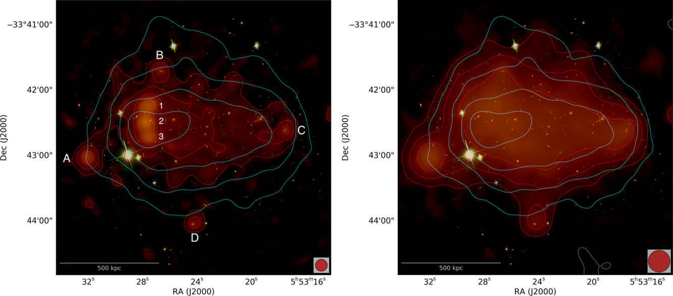
Figure 1. HST i,r,g image of MACSJ0553 with 943 MHz ASKAP radio emission and Chandra X-ray emission overlaid as contours. ASKAP emission is shown by red contours at levels  $[3, 6, 12, 24]\,\times\,\sigma$
. Smoothed Chandra X-ray contours are in cyan. Left: Our ASKAP image made with DDF after DD calibration (
$[3, 6, 12, 24]\,\times\,\sigma$
. Smoothed Chandra X-ray contours are in cyan. Left: Our ASKAP image made with DDF after DD calibration ( $\sigma = 20\,\mu$
Jy beam−1, restoring beam 11 arcsec
$\sigma = 20\,\mu$
Jy beam−1, restoring beam 11 arcsec  $\times$
11 arcsec). Right: Our ASKAP image made with DDF after point source subtraction and DD calibration (
$\times$
11 arcsec). Right: Our ASKAP image made with DDF after point source subtraction and DD calibration ( $\sigma = 25\,\mu$
Jy beam−1, restoring beam 20 arcsec
$\sigma = 25\,\mu$
Jy beam−1, restoring beam 20 arcsec  $\times$
20 arcsec). The red colour of the ASKAP emission is included for visualisation only. See text for imaging parameters.
$\times$
20 arcsec). The red colour of the ASKAP emission is included for visualisation only. See text for imaging parameters.
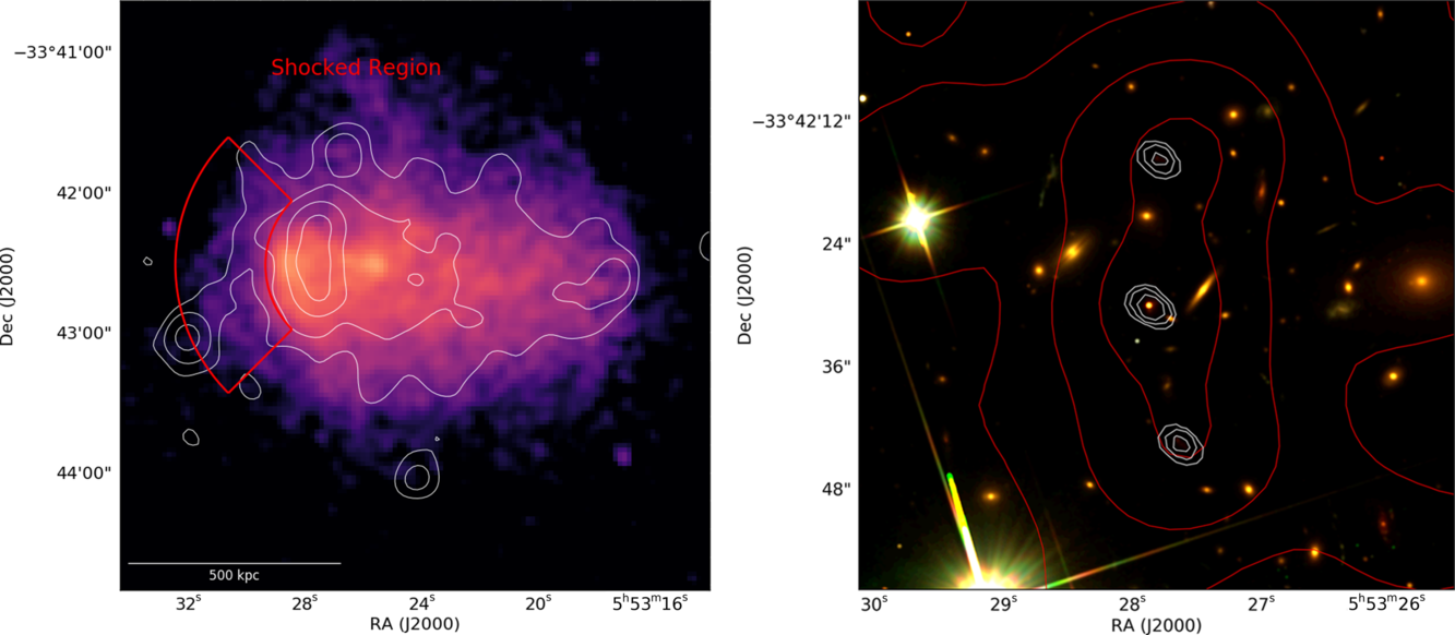
Figure 2. Left: Smoothed Chandra X-ray emission of MACSJ0553 with our ASKAP DD image overlaid as contours (levels are same as Figure 1: Left). The red region highlights the location of the shock detected in MACSJ0553 and is a reproduction from Pandge et al. (Reference Pandge2017). Right: HST i, r, g image of MACSJ0553 with VLA S-band radio emission and ASKAP 943 MHz radio emission overlaid as contours. VLA emission is shown by white contours  $[3, 6, 12, 24]\,\times\,\sigma$
where
$[3, 6, 12, 24]\,\times\,\sigma$
where  $\sigma = 10\,\mu$
Jy beam−1. ASKAP emission is shown by red contours
$\sigma = 10\,\mu$
Jy beam−1. ASKAP emission is shown by red contours  $[6, 12, 24]\,\times\,\sigma$
where
$[6, 12, 24]\,\times\,\sigma$
where  $\sigma = 25\,\mu$
Jy beam−1.
$\sigma = 25\,\mu$
Jy beam−1.
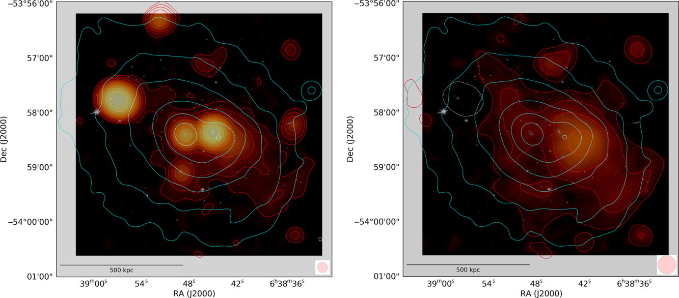
Figure 3. HST r image of AS0592 with ASKAP 1013 MHz radio emission and Chandra X-ray emission overlaid as contours. Left: our final image made with DDF ( $\sigma = 20\,\mu$
Jy beam−1, restoring beam 11 arcsec
$\sigma = 20\,\mu$
Jy beam−1, restoring beam 11 arcsec  $\times$
11 arcsec). Right: diffuse emission after subtracting compact emission imaged with a uvrange
$\times$
11 arcsec). Right: diffuse emission after subtracting compact emission imaged with a uvrange  ${>}1\,$
km (
${>}1\,$
km ( $\sigma = 25\,\mu$
Jy beam−1, restoring beam 20 arcsec
$\sigma = 25\,\mu$
Jy beam−1, restoring beam 20 arcsec  $\times$
20 arcsec). ASKAP emission in both images is shown by red contours at
$\times$
20 arcsec). ASKAP emission in both images is shown by red contours at  $[3, 6, 12, 24, 48, 96]\,\times\,\sigma$
and white dashed contours at
$[3, 6, 12, 24, 48, 96]\,\times\,\sigma$
and white dashed contours at  $[-2]\,\times\,\sigma$
. Smoothed Chandra X-ray contours as also shown in cyan. The red colour is for visualisation only. See text for imaging parameters.
$[-2]\,\times\,\sigma$
. Smoothed Chandra X-ray contours as also shown in cyan. The red colour is for visualisation only. See text for imaging parameters.
To confirm whether this emission was coming from one or more radio galaxies, we utilised high-resolution (configuration A) VLA S-band observations of the cluster. When overlaying our VLA image with a resolution of 2.5 arcsec  $\times$
1.2 arcsec on the HST optical image, it is clear that this emission is in fact produced by either three separate compact radio galaxies or by one radio galaxy with two hotspots (see Figure 2: Right). As an estimate from the colour and size of the optical counterparts, the source in the middle (2) appears to belong to a resident galaxy of the cluster, while the Northern (1) and Southern (3) radio sources appear to be associated with faint background galaxies; however, the N and S sources could possibly be equidistant hotspots from the AGN of the middle, resident galaxy. There are no reported redshifts available for these galaxies.
$\times$
1.2 arcsec on the HST optical image, it is clear that this emission is in fact produced by either three separate compact radio galaxies or by one radio galaxy with two hotspots (see Figure 2: Right). As an estimate from the colour and size of the optical counterparts, the source in the middle (2) appears to belong to a resident galaxy of the cluster, while the Northern (1) and Southern (3) radio sources appear to be associated with faint background galaxies; however, the N and S sources could possibly be equidistant hotspots from the AGN of the middle, resident galaxy. There are no reported redshifts available for these galaxies.
To measure the integrated flux density of the radio halo in MACSJ0553, we performed a point source subtraction of the three embedded AGN. Our method for subtraction is described in Section 2.3. In the full bandwidth AKSAP image, it is apparent that there are some additional, very faint point sources around the border of the halo emission (A, B, C, and D in Figure 1: Left). Three of these very faint, compact sources (B, C, and D) appear to coincide with disk-hosting galaxies and may come from very small-scale Seyfert jets. One point source to the East (A) is beyond the edge of the HST optical image, so we do not know whether it belongs to a foreground or background galaxy. However, none of these faint point sources appears in any of our six sub-band images, nor in our GMRT or VLA images, and could not be measured with the Aegean (Hancock et al. Reference Hancock, Murphy, Gaensler, Hopkins and Curran2012; Hancock, Trott, & Hurley-Walker Reference Hancock, Trott and Hurley-Walker2018) source detection software, so they were not modelled or subtracted.
In Figure 1: Right, we show the radio halo emission imaged after subtracting the three N-S compact AGN (1, 2, and 3) and subsequent DD calibration. To capture emission on larger scales, this image was made with a Briggs robust setting of  $-$
0.75 and a restoring beam of 20 arcsec. We measure the integrated flux density of the radio halo within a polygon region marked by the
$-$
0.75 and a restoring beam of 20 arcsec. We measure the integrated flux density of the radio halo within a polygon region marked by the  $3\sigma$
contour lineFootnote i, where
$3\sigma$
contour lineFootnote i, where  $\sigma = 25\,\mu$
Jy beam−1. The halo has a flux density of
$\sigma = 25\,\mu$
Jy beam−1. The halo has a flux density of  $S_{943}\,{\rm MHz} = 12.22 \pm 1.37$
mJy and the largest linear size (LLS) is 0.9 Mpc. The error is calculated from the estimated error on the flux scale (10%) and from the error in measuring the flux density when considering the rms noise (
$S_{943}\,{\rm MHz} = 12.22 \pm 1.37$
mJy and the largest linear size (LLS) is 0.9 Mpc. The error is calculated from the estimated error on the flux scale (10%) and from the error in measuring the flux density when considering the rms noise ( $\pm\,0.17$
mJy). The halo traces the X-ray emission quite well, filling the full inner volume of the cluster; however, it is slightly more elongated from East to West and shortened from North to South.
$\pm\,0.17$
mJy). The halo traces the X-ray emission quite well, filling the full inner volume of the cluster; however, it is slightly more elongated from East to West and shortened from North to South.
We also derive the integrated spectral index estimate of the radio halo by comparing the diffuse emission (after point source subtraction) as seen by the GMRT at 323 MHz to the diffuse emission as seen by ASKAP. To do this, we made images with uniform weighting and the same minimum uv range of  $100\,\lambda$
, regridded the GMRT image to the ASKAP image, and smoothed both of the images to the same beam size (22 arcsec). From these images, we measure the flux density within the same region, tracing the
$100\,\lambda$
, regridded the GMRT image to the ASKAP image, and smoothed both of the images to the same beam size (22 arcsec). From these images, we measure the flux density within the same region, tracing the  $3\sigma$
contour line of the 943 MHz AKSAP image. We find that the radio halo has a flux density of
$3\sigma$
contour line of the 943 MHz AKSAP image. We find that the radio halo has a flux density of  $7.61 \pm 0.87$
mJy at 943 MHz and
$7.61 \pm 0.87$
mJy at 943 MHz and  $22.02 \pm 0.92$
mJy at 323 MHz in these uniform-weighted images, and therefore we estimate the spectral index of the halo to be
$22.02 \pm 0.92$
mJy at 323 MHz in these uniform-weighted images, and therefore we estimate the spectral index of the halo to be  $\alpha_{323}^{943} = -0.99 \pm 0.12$
.
$\alpha_{323}^{943} = -0.99 \pm 0.12$
.
3.2. Abell S0592
Our ASKAP image at 1013 MHz after DD calibration of AS0592 (see Figure 3: Left) shows diffuse intracluster emission that has not been previously reported in the literature. There are four bright, and somewhat extended, radio galaxies embedded in the diffuse emission. One of these radio galaxies, at the cluster centre, has a slightly extended lobe that points toward the West. This more extended counterpart of the central radio galaxy appears to bleed into the diffuse emission in the ICM.
Our image after modelling and subtracting the bright cluster radio galaxies is shown on the right in Figure 3. To better capture diffuse emission, this image was made with a Briggs robust setting of  $-$
0.75 and a restoring beam of 20 arcsec. As explained in Sections 2.3 and 4.1, we attempted several techniques to properly subtract the radio galaxy emission in this cluster and found that the best result was to model and subtract the emission using the DDF imager after applying DD calibration solutions. The resulting image does leave a hole (negative artefact, marked by the dashed white contour line in Figure 3: Right) where the brightest radio galaxy, to the North-East, was subtracted. The diffuse intracluster emission faintly extends within this North-East region of the cluster, so we expect that our flux density measurement in this region will be an underestimation. However, the central radio galaxy with the extended Western lobe appears to leave some residual emission after subtraction, so the flux density measurement in this region will likely be an overestimation. It is difficult to quantify the amount of error that this imperfect subtraction introduces, but we assume a liberal estimate that it is on the order of
$-$
0.75 and a restoring beam of 20 arcsec. As explained in Sections 2.3 and 4.1, we attempted several techniques to properly subtract the radio galaxy emission in this cluster and found that the best result was to model and subtract the emission using the DDF imager after applying DD calibration solutions. The resulting image does leave a hole (negative artefact, marked by the dashed white contour line in Figure 3: Right) where the brightest radio galaxy, to the North-East, was subtracted. The diffuse intracluster emission faintly extends within this North-East region of the cluster, so we expect that our flux density measurement in this region will be an underestimation. However, the central radio galaxy with the extended Western lobe appears to leave some residual emission after subtraction, so the flux density measurement in this region will likely be an overestimation. It is difficult to quantify the amount of error that this imperfect subtraction introduces, but we assume a liberal estimate that it is on the order of  ${\sim}15\%$
.
${\sim}15\%$
.
Due to its LLS of 1.04 Mpc, we classify this diffuse emission as a giant radio halo. From our source-subtracted DD ASKAP image, we measure the flux density of the radio halo within a region marked by the  $3\sigma$
contour line where
$3\sigma$
contour line where  $\sigma = 25\,\mu$
Jy beam−1. We find that the integrated flux density is
$\sigma = 25\,\mu$
Jy beam−1. We find that the integrated flux density is  $S_{1013\,{\rm MHz}} = 9.95 \pm 2.16$
mJy. The error is calculated from the estimated error on the flux scale (5%), the error in measuring the flux density when considering the rms noise (
$S_{1013\,{\rm MHz}} = 9.95 \pm 2.16$
mJy. The error is calculated from the estimated error on the flux scale (5%), the error in measuring the flux density when considering the rms noise ( $\pm\,0.18$
mJy), and an estimate of error due to imperfect source subtraction (15%).
$\pm\,0.18$
mJy), and an estimate of error due to imperfect source subtraction (15%).
We were also able to image some diffuse emission in this cluster with ATCA observations. As some of the cluster radio galaxies showed small-scale extended structure in the ATCA data, we imaged the data initially using a balanced Briggs weighting with the robust parameter set to 0.0. No large-scale, diffuse emission was modelled at this stage, and the CLEAN components were subtracted before re-imaging with a natural visibility weighting. A natural weighting was required to maximise the sensitivity to the extended diffuse structure barely significant in the robust 0.0 residuals. The residuals in this naturally weighted image coincide with the radio halo detected in the ASKAP image. The residual emission after source subtraction is only significant in the full-bandwidth image centred at 2.215 GHz. The flux density of the diffuse emission measured within a region tracing the  $3\sigma$
contour line, where
$3\sigma$
contour line, where  $\sigma = 120\,\mu$
Jy beam−1, is
$\sigma = 120\,\mu$
Jy beam−1, is  $S_{2215}\,{\rm MHz} = 3.3 \pm 0.4$
mJy. The error on the flux comes from a
$S_{2215}\,{\rm MHz} = 3.3 \pm 0.4$
mJy. The error on the flux comes from a  ${\sim}2\%$
error due to calibration of ATCA data for the 16 cm band and the error from the rms. We are unable to quantify the error introduced from source subtraction.
${\sim}2\%$
error due to calibration of ATCA data for the 16 cm band and the error from the rms. We are unable to quantify the error introduced from source subtraction.
We derive an integrated spectral index estimate of the radio halo in AS0592 by comparing the diffuse emission as seen by ASKAP to the diffuse emission as seen by ATCA. The spectral index estimate was calculated using measurements from our source-subtracted DD-calibrated ASKAP image and our natural-weight ATCA image. Since the spectral index should ideally be calculated from flux density measurements that are taken from images made with uniform weighting, we expect that our value will be biased, but we could not capture any diffuse emission by imaging the ATCA data with a uniform weight. The spectral index of the halo is estimated to be  $\alpha^{2215}_{1013} = -1.41 \pm 0.25$
. The error on this value comes from the error on the flux density alone, since we are unable to quantify the error due to the different weighting schemes.
$\alpha^{2215}_{1013} = -1.41 \pm 0.25$
. The error on this value comes from the error on the flux density alone, since we are unable to quantify the error due to the different weighting schemes.
In Figure 4, we present our X-ray image of AS0592 from archival Chandra data with our ASKAP DD image (after source subtraction) overlaid as contours. It is apparent that this system has two X-ray peaks with a morphology indicating a Bullet-type merger. The central peak is the brightest, and the second, dimmer peak to the West represents the ‘bullet’. The radio halo in this cluster is more offset from the X-ray gas, filling the South-Western volume of the ICM, as seen in projection, and it also follows quite closely with the central radio galaxies. The SW border of the radio halo appears to have a more linear edge, roughly coincident with the surface brightness (SB) edge reported by Botteon et al. (Reference Botteon, Gastaldello and Brunetti2018). Because they measured a steep temperature drop across this edge, Botteon et al. (Reference Botteon, Gastaldello and Brunetti2018) claim the presence of a shock. We construct a SB radial profile in a wider regionFootnote j across the SW portion of the cluster and compare it to the profile from Botteon et al. (Reference Botteon, Gastaldello and Brunetti2018), which was measured over a narrower region. In Figure 5, the X-ray SB profiles, constructed using the proffit software (Eckert, Molendi, & Paltani Reference Eckert, Molendi and Paltani2011), are compared to the radio SB profile over the same region. The radio SB profile is computed by azimuthally averaging the SB in radially equal bins equivalent to the size of the synthesised beam (22 arcsec). Uncertainties in the azimuthally averaged SB are estimated via  $\langle\sigma_\mathrm{rms}\rangle/\sqrt{N_\mathrm{beam}}$
, where
$\langle\sigma_\mathrm{rms}\rangle/\sqrt{N_\mathrm{beam}}$
, where  $\langle\sigma_\mathrm{rms}\rangle$
is the mean image rms in the bin, and
$\langle\sigma_\mathrm{rms}\rangle$
is the mean image rms in the bin, and  $N_\mathrm{beam}$
is the number of independent beams covering the bin. In Figure 5, it is apparent that the azimuthally averaged SB in radio falls off at a similar rate to the X-ray SB.
$N_\mathrm{beam}$
is the number of independent beams covering the bin. In Figure 5, it is apparent that the azimuthally averaged SB in radio falls off at a similar rate to the X-ray SB.
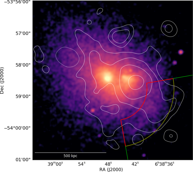
Figure 4. Smoothed Chandra X-ray emission of AS0592 with our 1013 MHz ASKAP DD image, after source subtraction, overlaid as contours (levels are same as Figure 3: Right.) Panda annulus shows where surface brightness was measured for a radial profile. The yellow curve indicates the surface brightness (SB) edge.
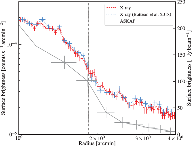
Figure 5. The azimuthally averaged SB in our radio AKSAP map is compared to the SB in X-rays. One radio SB measurement is made per beam size (22 arcsec) over 4 arcmin. The dashed vertical line marks the edge corresponding to a jump in SB. Note that radial uncertainties correspond to bin widths.
4. Discussion
4.1. Subtraction with DDF
Subtracting the bright and more extended sources in AS0592 proved to be more of a challenge than subtracting the point sources in MACSJ0553. Most methods of source subtraction involve modelling sources from a source detection software (e.g. PYBDSF (Mohan & Rafferty Reference Mohan and Rafferty2015) or Aegean (Hancock et al. Reference Hancock, Trott and Hurley-Walker2018)) or from the CLEAN components of an image. The brighter AGN in AS0592 were causing slight artefacts that appeared as rings in the ASKAPsoft image. Modelling and subtracting these sources prior to DD calibration would leave those ring-type artefacts in the final image, as well as remove potential directional calibrators for this region of the sky. By modifying our DD pipeline and inserting a customised mask, we were able to make an image of the compact AGN emission only and model and subtract the CLEAN components of that image from the calibrated visibilities. We then continued to run DDF once more on the new subtracted data column, while applying the same directional calibration solutions, this time including all baselines above 60 m and including a customised mask to cover diffuse emission on the scale of the galaxy cluster. The resulting image is the remaining diffuse emission, after modelling and subtracting the compact AGN with directional calibration applied. Unfortunately, we were unable to prevent a negative artefact from occurring where the brightest radio galaxy was subtracted. We attempted to mitigate this effect by raising the CLEAN threshold on the compact image, but found that too much flux was left remaining post-subtraction.
The central radio galaxy with an extended Western lobe does appear to have emission on the same scales as the radio halo. By decreasing the minimum UV-range in the compact image, more of this extended component could be modelled and subtracted, but it was our opinion that this could possibly remove halo-related emission as well. Therefore, we only modelled and subtracted emission on scales less than 250 kpc. With only the ASKAP and ATCA observations of this cluster, it is not possible to discern how much flux in our subtracted, diffuse emission image is contributed by the central AGN. When modelling the sources as Gaussians, measuring integrated flux densities over sub-band images, and using Subtrmodel (as was done for MACSJ0553), the remaining image contained more prominent negative artefacts. Modelling the sources through the DDF imager’s Predict function yielded the best result. These methods and results proved that our DD pipeline could be easily expanded to complete more specific tasks for science-related analysis, specifically in utilising additional options available in the DDF package.
4.2. On the absence of radio relics
Although MACSJ0553 is in merging state, after core passage, and a shock and cold front have been detected in X-rays, there is no detectable radio shock emission. The absence of a radio counterpart associated with a confirmed shock has been seen in some other clusters, such as in MACS J0744.9+3927 (Wilber et al. Reference Wilber2018b). Following the method for calculating shock acceleration efficiency as presented in Wilber et al. (Reference Wilber2018b) we carry out the same calculations here for the shock detected in MACSJ0553 to determine whether this shock would be able to generate a detectable radio relic.
Taking the parameters of the shock wave as measured by Pandge et al. (Reference Pandge2017)—a Mach number of  $\mathcal{M} = 1.33$
and shock velocityFootnote k
$\mathcal{M} = 1.33$
and shock velocityFootnote k $V_{\rm sh}=1892$
km s−1—and the non-detection of a radio relic, we can compute an upper limit on the particle acceleration efficiency. Comparing the dissipated kinetic power at the shock to the total power in the radio emissionFootnote l, we can estimate the acceleration efficiency using equation (2) in Botteon et al. (Reference Botteon, Gastaldello, Brunetti and Dallacasa2016):
$V_{\rm sh}=1892$
km s−1—and the non-detection of a radio relic, we can compute an upper limit on the particle acceleration efficiency. Comparing the dissipated kinetic power at the shock to the total power in the radio emissionFootnote l, we can estimate the acceleration efficiency using equation (2) in Botteon et al. (Reference Botteon, Gastaldello, Brunetti and Dallacasa2016):
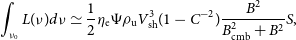 \begin{equation}\int_{\nu_{0}} L(\nu) d\nu \simeq \frac{1}{2} \eta_{\rm e} \Psi \rho_{\rm u} V_{\rm sh}^{3} (1 - C^{-2}) \frac{B^{2}}{B_{\rm cmb}^{2} + B^{2}} S ,\end{equation}
where  $\eta_{\rm e}$
is the acceleration efficiency,
$\eta_{\rm e}$
is the acceleration efficiency,  $\rho_{\rm u}$
is the upstream density,
$\rho_{\rm u}$
is the upstream density,  $V_{\rm sh}$
is the shock velocity, C is the compression factor which is related to the Mach number via
$V_{\rm sh}$
is the shock velocity, C is the compression factor which is related to the Mach number via  $C = 4 \mathcal{M}^{2} / (\mathcal{M}^{2} + 3)$
, B is the magnetic field strength and
$C = 4 \mathcal{M}^{2} / (\mathcal{M}^{2} + 3)$
, B is the magnetic field strength and  $B_{\rm cmb} = 3.25(1+z)^2$
, S is the surface area of the shockFootnote m, and
$B_{\rm cmb} = 3.25(1+z)^2$
, S is the surface area of the shockFootnote m, and  $\Psi$
is the ratio of the energy injected in electrons emitting over the full spectrum versus electrons emitting in radio wavelengths, given by
$\Psi$
is the ratio of the energy injected in electrons emitting over the full spectrum versus electrons emitting in radio wavelengths, given by
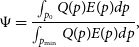 \begin{equation}\Psi = \frac{\int_{p_{0}} Q(p) E(p) dp}{\int_{p_{\rm min}} Q(p) E(p) dp} ,\end{equation}
where  $Q(p) \propto p^{-\delta_{\rm inj}}$
and
$Q(p) \propto p^{-\delta_{\rm inj}}$
and  $\delta_{\rm inj} = 2(\mathcal{M}^{2} + 1)/(\mathcal{M}^{2} - 1)$
(Blandford & Eichler Reference Blandford and Eichler1987). The momentum,
$\delta_{\rm inj} = 2(\mathcal{M}^{2} + 1)/(\mathcal{M}^{2} - 1)$
(Blandford & Eichler Reference Blandford and Eichler1987). The momentum,  $p_0$
, is the momentum associated with electrons that emit the characteristic frequency of the synchrotron emission,
$p_0$
, is the momentum associated with electrons that emit the characteristic frequency of the synchrotron emission,  $\nu_0=p_0^2 e B /2\pi m_{\rm e}^3c^3$
. Here,
$\nu_0=p_0^2 e B /2\pi m_{\rm e}^3c^3$
. Here,  $m_{\rm e}$
is the electron mass, e its charge, and c the speed of light. We used the value from Table 5 in Pandge et al. (Reference Pandge2017) for the upstream density in the shocked region (
$m_{\rm e}$
is the electron mass, e its charge, and c the speed of light. We used the value from Table 5 in Pandge et al. (Reference Pandge2017) for the upstream density in the shocked region ( $\rho_{\rm u} = 0.3 \times 10^{-4}\,$
cm−3), and since the magnetic field in this cluster is not known we assume a value of
$\rho_{\rm u} = 0.3 \times 10^{-4}\,$
cm−3), and since the magnetic field in this cluster is not known we assume a value of  $B=1\,\mu$
G. For the minimum momentum in the denominator,
$B=1\,\mu$
G. For the minimum momentum in the denominator,  $p_{\rm min}$
, we consider two cases: (1) a low value of
$p_{\rm min}$
, we consider two cases: (1) a low value of  $p_{\rm min} = 0.1 m_{\rm e}c$
representing electrons accelerated from the thermal pool, and (2) a higher value of
$p_{\rm min} = 0.1 m_{\rm e}c$
representing electrons accelerated from the thermal pool, and (2) a higher value of  $p_{\rm min} = 100 m_{e}c$
representing a population of relativistic seed electrons. However, we find that in both cases the efficiency has to be unrealistically high,
$p_{\rm min} = 100 m_{e}c$
representing a population of relativistic seed electrons. However, we find that in both cases the efficiency has to be unrealistically high,  $\gg 100\%$
, and we cannot infer an upper bound for
$\gg 100\%$
, and we cannot infer an upper bound for  $\eta_{\rm e}$
. This is likely due to the fact that the upstream density in the shocked region is very low. A relic is not observed, and given these acceleration efficiency calculations a relic would not be expected to form.
$\eta_{\rm e}$
. This is likely due to the fact that the upstream density in the shocked region is very low. A relic is not observed, and given these acceleration efficiency calculations a relic would not be expected to form.
The clear Bullet-type merging cluster AS0592 also appears to host a shock, as measured by Botteon et al. (Reference Botteon, Gastaldello and Brunetti2018) and confirmed in our X-ray SB profile. Of the radio emission in this region, there does not appear to be any substantial brightening or structural morphology that resembles a radio relic. Instead the radio halo exhibits a linear edge roughly coincident with the location of the shock. There have been several cases where borders of radio halos are observed to coincide with, or be bounded by, SB edges detected in the thermal X-ray emission (e.g. Brown & Rudnick Reference Brown and Rudnick2011; Markevitch et al. Reference Markevitch, Govoni, Brunetti and Jerius2005; Shimwell et al. Reference Shimwell, Brown, Feain, Feretti, Gaensler and Lage2014; Vacca et al. Reference Vacca, Feretti, Giovannini, Govoni, Murgia, Perley and Clarke2014; Wang, Giacintucci, & Markevitch Reference Wang, Giacintucci and Markevitch2018; van Weeren et al. Reference van Weeren2016b). Compression from the shock in this region would only be confirmed through polarisation measurements and high-resolution spectral maps. As posed by van Weeren et al. (Reference van Weeren2019), there could be turbulence after the passage of a shock, such that a previously formed radio relic now appears blended with the halo emission. We cannot compute the acceleration efficiency of the shock because it is not possible to define a region of radio emission that is potentially generated by the shock. This halo-shock connection in AS0592 is very similar to the case in Abell 520, where a Bullet-type shock front is also discovered to be coincident with the SW edge of a halo, although there the radio emission increases more sharply over the shock front from West to East (upstream to downstream) (Hoang et al. Reference Hoang2019).
For both clusters, the shocks detected are relatively weak. It has been proven that stronger shocks ( $\mathcal{M} = 3-4$
) are typically necessary to produce observable radio relics (Hong et al. Reference Hong, Ryu, Kang and Cen2014). With the results of this paper, we confirm two more cases where merger-induced shocks do not have clear radio counterparts.
$\mathcal{M} = 3-4$
) are typically necessary to produce observable radio relics (Hong et al. Reference Hong, Ryu, Kang and Cen2014). With the results of this paper, we confirm two more cases where merger-induced shocks do not have clear radio counterparts.
4.3. On the origins of the radio halos
Although the masses estimated from SPT observations of the two clusters are relatively similar, the Planck estimated masses of these clusters differ substantially, with a larger discrepancy for AS0592: the mass estimate from SPT observations ( $M_{500} = 11.29^{+1.36}_{-1.10} \times 10^{14}$
M
$M_{500} = 11.29^{+1.36}_{-1.10} \times 10^{14}$
M $_{\odot}$
) is almost twice the mass estimated from Planck observations (
$_{\odot}$
) is almost twice the mass estimated from Planck observations ( $M_{500} = 6.83^{+0.34}_{-0.31} \times 10^{14}$
M
$M_{500} = 6.83^{+0.34}_{-0.31} \times 10^{14}$
M $_{\odot}$
). In a study of mass calibration for SPT observations, Bocquet et al. (Reference Bocquet2015) found that the average cluster masses in a catalogue of 100 SPT clusters were consistently greater (by
$_{\odot}$
). In a study of mass calibration for SPT observations, Bocquet et al. (Reference Bocquet2015) found that the average cluster masses in a catalogue of 100 SPT clusters were consistently greater (by  ${\sim}32\%$
) than their previous study (Reichardt et al. Reference Reichardt2013), likely due to updated cosmological data. However, there are no published studies explicitly addressing discrepancies between Planck and SPT cluster masses.
${\sim}32\%$
) than their previous study (Reichardt et al. Reference Reichardt2013), likely due to updated cosmological data. However, there are no published studies explicitly addressing discrepancies between Planck and SPT cluster masses.
In Figure 6, we plot the halos in MACSJ0553 and AS0592 by their power at 1.4 GHzFootnote n versus their cluster mass as listed by both the SPT and Planck catalogues and compare them to the  $P-M$
correlation reproduced from Martinez Aviles et al. (Reference Martinez Aviles2016). In this plot, it is easy to see that although the SPT masses of the clusters are very similar, their radio powers are very different, with the halo in MACSJ0553 being much more luminous. Given the SPT mass estimates, both of the halos also lie far outside of the current
$P-M$
correlation reproduced from Martinez Aviles et al. (Reference Martinez Aviles2016). In this plot, it is easy to see that although the SPT masses of the clusters are very similar, their radio powers are very different, with the halo in MACSJ0553 being much more luminous. Given the SPT mass estimates, both of the halos also lie far outside of the current  $P-M$
correlation at 1.4 GHz. If, however, one considers the Planck estimated mass, the halo powers agree more closely with the correlation that suggests that a lower mass cluster will host a lower luminosity radio halo.
$P-M$
correlation at 1.4 GHz. If, however, one considers the Planck estimated mass, the halo powers agree more closely with the correlation that suggests that a lower mass cluster will host a lower luminosity radio halo.
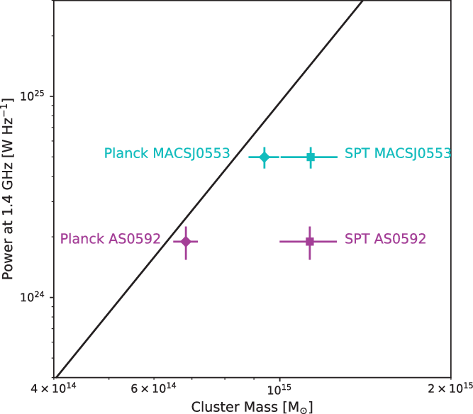
Figure 6. The powers of the halos in MACSJ0553 and AS0592 are extrapolated to 1.4 GHz and plotted against their differing mass estimates from SPT and Planck. The derived fit, or  $P-M$
correlation, for a sample of halos with flux measured at 1.4 GHz is shown as a black line, from Martinez Aviles et al. (Reference Martinez Aviles2016).
$P-M$
correlation, for a sample of halos with flux measured at 1.4 GHz is shown as a black line, from Martinez Aviles et al. (Reference Martinez Aviles2016).
In an evolutionary simulation, Donnert et al. (Reference Donnert, Dolag, Brunetti and Cassano2013) found that the X-ray luminosity of a merging cluster will change over the lifetime of the merger, and that the power emitted by a merger-generated radio halo is transient, rising and falling along the  $P-L$
correlation. This has two interesting implications: 1) because of its transience, X-ray luminosity is not an entirely reliable property for measuring cluster mass, and 2) if AS0592 and MACSJ0533 have similar masses, as indicated by the SPT-SZ measurements, the differences in the halo powers may be connected to the evolutionary state of the mergers.
$P-L$
correlation. This has two interesting implications: 1) because of its transience, X-ray luminosity is not an entirely reliable property for measuring cluster mass, and 2) if AS0592 and MACSJ0533 have similar masses, as indicated by the SPT-SZ measurements, the differences in the halo powers may be connected to the evolutionary state of the mergers.
As seen in our AKSAP image, the radio halo in MACSJ0553 fills the ICM and traces the X-ray emission of the cluster very well, indicating that the full volume of the ICM contains ultra-relativistic electrons. Except for the small point-source AGN coinciding with a single cluster galaxy, there does not appear to be any other radio emitting galaxies in the cluster environment. This begs the question of the origin of such a uniform population of CRe in this cluster. A calculation made by Bonafede et al. (Reference Bonafede2012) was that the timescale after core passage in MACSJ0553 would not allow sufficient time for a halo of that size to generate from turbulent re-acceleration alone. These clues lend support to the hadronic model, in which ultra-relativistic electrons can be generated by the collisions of thermal and cosmic-ray protons in the ICM. The luminosity of the halo and the flatter spectral index are also more in line with the hadronic model. It would be interesting to look at sensitive  $\gamma$
-ray observations of this cluster to determine whether its
$\gamma$
-ray observations of this cluster to determine whether its  $\gamma$
-luminosity is above the average upper limit of other clusters.
$\gamma$
-luminosity is above the average upper limit of other clusters.
In contrast, AS0592 contains several bright radio galaxies that are injecting relativistic electrons into the surrounding environment. The radio halo in AS0592 tightly hugs the regions where the radio galaxies are present, and the central Western radio galaxy even appears to have lobe emission that bleeds into the emission of the halo. Given its morphology and proximity to the cluster radio galaxies, it is probable that the radio halo was generated from a contributed population of AGN seed, or remnant, electrons, which have then been ‘boosted’ by the turbulence of the cluster merger. We suspect that observations from the upcoming EMU survey will reveal many more examples where diffuse cluster sources are clearly fed by remnant AGN emission.
The turbulent re-acceleration model predicts that radio halos will be generated by a larger population of lower-energy electrons, yielding a steeper spectral index (Brunetti et al. Reference Brunetti2008). Our spectral index estimate for the halo in AS0592 almost qualifies as ultra-steep (where  $\alpha \leq -1.5$
), but we are wary of regarding this value as accurate because it was difficult to recover the diffuse emission in this cluster with higher frequencies. We were also unable to utilise low-frequency MWA observations due to the lower resolution of the interferometer and significant source-blending, as seen in GLEAM images. High-resolution, low-frequency observations would be needed to accurately subtract the compact radio galaxies and measure the flux density of the radio halo in this cluster. Nonetheless, due to its more irregular morphology, lower luminosity, and association with nearby galaxies, we argue that the halo in AS0592 falls more in line with the turbulent re-acceleration model.
$\alpha \leq -1.5$
), but we are wary of regarding this value as accurate because it was difficult to recover the diffuse emission in this cluster with higher frequencies. We were also unable to utilise low-frequency MWA observations due to the lower resolution of the interferometer and significant source-blending, as seen in GLEAM images. High-resolution, low-frequency observations would be needed to accurately subtract the compact radio galaxies and measure the flux density of the radio halo in this cluster. Nonetheless, due to its more irregular morphology, lower luminosity, and association with nearby galaxies, we argue that the halo in AS0592 falls more in line with the turbulent re-acceleration model.
5. Conclusions
Early science survey observations from ASKAP were made public through CASDA in 2019. Examining the data, we found signs of diffuse emission associated with two high-mass, merging clusters: MACSJ0553 and AS0592. We pulled the calibrated data sets covering these clusters from CASDA and performed further processing using our own pipeline, implementing the software packages DDFacet and killMS (Tasse et al. Reference Tasse2018) to calibrate against directional errors in the data.
From our DD ASKAP images, we confirm the presence of a giant radio halo in MACSJ0553 (previously detected by Bonafede et al. Reference Bonafede2012) and announce the discovery of a giant radio halo in AS0592. The halos have a similar LLS of  ${\sim}1\,$
Mpc but differ in radio luminosity despite the similar masses of the clusters. We find the flux densities of the halos to be
${\sim}1\,$
Mpc but differ in radio luminosity despite the similar masses of the clusters. We find the flux densities of the halos to be  $S_{943}\,{\rm MHz} = 12.22 \pm 1.37$
mJy and
$S_{943}\,{\rm MHz} = 12.22 \pm 1.37$
mJy and  $S_{1013\,{\rm MHz}} = 9.95 \pm 2.16$
mJy for MACSJ0553 and AS0592, respectively. In comparing measurements at other frequencies, we estimate the integrated spectral indices to be
$S_{1013\,{\rm MHz}} = 9.95 \pm 2.16$
mJy for MACSJ0553 and AS0592, respectively. In comparing measurements at other frequencies, we estimate the integrated spectral indices to be  $\alpha_{323}^{943} = -0.99 \pm 0.12$
for the halo in MACSJ0553 and
$\alpha_{323}^{943} = -0.99 \pm 0.12$
for the halo in MACSJ0553 and  $\alpha^{2215}_{1013} = -1.41 \pm 0.25$
for the halo in AS0592.
$\alpha^{2215}_{1013} = -1.41 \pm 0.25$
for the halo in AS0592.
The halo in MACSJ0553 traces the thermal emission of the cluster extremely well and does not appear to be fed by seed electrons from any cluster AGN. Due to its size, morphology, high luminosity, and flatter spectral index, we argue that this halo falls more in line with the hadronic model. In contrast, the radio halo in AS0592 is more irregular in shape and does not fill the full volume of the cluster, but instead closely traces the location of resident radio galaxies. We argue that these cluster radio galaxies contribute a population of seed electrons that have been re-energised by the major merger of the cluster. Due to its morphology, lower radio luminosity, its association with radio galaxies in the cluster, and the fact that the halo is offset from the X-ray gas, we argue that this halo falls more in line with the turbulent re-acceleration model.
As indicated by their thermal X-ray emission, both clusters have independently undergone major mergers and are in the phase after core passage. Both clusters also show SB edges in their X-ray radial profiles, corresponding to shocks as confirmed by a jump in temperature. However, neither of the clusters host a radio shock. While the merger shocks have relatively low mach numbers, the upstream particle density in MACSJ0553 is too small to produce a radio shock. In AS0592, the shock boundary coincides roughly with the edge of the radio halo.
It is compelling to consider the differences in the halos for two clusters that have such similar merger dynamics, mass, and X-ray properties. This reinforces our uncertainty regarding the origin of these sources. High-resolution, low-frequency observations of these clusters will help to constrain the spectral indices of the radio halos, and, in conjunction with more sensitive  $\gamma$
-ray observations, may provide more clarity on their distinctive origins.
$\gamma$
-ray observations, may provide more clarity on their distinctive origins.
Acknowledgements
The Australian SKA Pathfinder is part of the Australia Telescope National Facility which is managed by CSIRO. Operation of ASKAP is funded by the Australian Government with support from the National Collaborative Research Infrastructure Strategy. ASKAP uses the resources of the Pawsey Supercomputing Centre. Establishment of ASKAP, the Murchison Radio-astronomy Observatory, and the Pawsey Supercomputing Centre are initiatives of the Australian Government, with support from the Government of Western Australia and the Science and Industry Endowment Fund. We acknowledge the Wajarri Yamatji people as the traditional owners of the Observatory site. This paper includes archived data obtained through the CSIRO ASKAP Science Data Archive, CASDA (http://data.csiro.au). The ATCA is part of the Australia Telescope National Facility which is funded by the Australian Government for operation as a National Facility managed by CSIRO. This paper includes archived data obtained through the Australia Telescope Online Archive (http://atoa.atnf.csiro.au). This work was supported by resources provided by the Pawsey Supercomputing Centre with funding from the Australian Government and the Government of Western Australia. We acknowledge and thank the builders of ASKAPsoft. AGW acknowledges the Hamburger Sternwarte for its computing resources. AGW thanks Aidan Hotan, Ron Ekers, Dave McConnell, Marcus Brüggen, and Andrea Botteon. SWD acknowledges an Australian Government Research Training Program scholarship administered through Curtin University. In memory of Jean-Pierre Macquart.


