


Food acquisition surveys have been used to track habitual food and drink consumption, examine patterns of food acquisition by different demographic subgroups and understand food security( Reference Ricciuto and Tarasuk 1 – Reference Griffin and Sobal 3 ). Estimates produced by these surveys provide valuable insight for the drafting and modification of policies and programmes designed to promote healthy eating and better lifestyles, and for assisting groups of people who are identified as being food insecure.
A recent survey by the US Department of Agriculture (USDA), the National Household Food Acquisition and Purchase Survey (FoodAPS), represents such an effort to generate these important estimates( 4 ). FoodAPS is the first nationally representative survey in the USA to collect detailed week-long information on all household food acquisitions along with other related indicators such as food security, income, employment and participation in food assistance programmes. FoodAPS is a comprehensive survey that involved both face-to-face interviewing and a 7 d diary survey component to be completed by all members of the sampled households.
The data collection protocol for FoodAPS required an extensive amount of involvement from human interviewers. Interviewers were responsible for training the household to record their food acquisitions throughout the survey period using the diary. They were also responsible for conducting the initial and final face-to-face interviews. It is therefore important to understand if survey outcomes in FoodAPS (e.g. measures of food security, missing income reports) tend to have distributions that vary across interviewers, above and beyond any variance introduced by the quality of the instruments or the features of the respondents. Despite nearly a century of research into the potentially negative effects of human interviewers on survey data collection( Reference West and Blom 5 ), we are unaware of any prior research that has evaluated these effects in the context of food acquisition surveys. If these effects exist, they may have an impact on the conclusions drawn from using these data. The objective of the present study was to examine these systematic effects of interviewers on several different data collection outcomes in the FoodAPS.
Interviewer effects and FoodAPS
Researchers have long studied the variable effects of interviewers on different types of survey errors under the term ‘interviewer effects’( Reference West and Blom 5 – Reference West and Olson 12 ). We define ‘interviewer effect’ here as the systematic effect of a particular interviewer on a given survey process (e.g. acquiring consent for record linkage) or outcome (e.g. insurance coverage, health). These effects may vary among different interviewers, giving rise to the term ‘interviewer variance’. Interviewers have been found to use different techniques to list household members to select a respondent, as well as different techniques to identify and list occupied homes in a given area for sample selection( Reference West and Blom 5 , Reference Eckman and Kreuter 6 ). This can introduce variable population coverage errors among interviewers if this listing is used to construct a sampling frame to draw samples from, as different interviewers will use different metrics to judge if a house is ‘occupied’( Reference Eckman and Kreuter 6 ). Interviewers have frequently been found to vary in terms of their achieved response rates( Reference West and Blom 5 ) and some studies have presented evidence of interviewer variability in rates of consent for additional data collection or linkage of respondents’ answers to other administrative data sources( Reference O’Muircheartaigh and Campanelli 7 , Reference Korbmacher and Schroeder 8 ). Finally, interviewers have frequently been found to introduce varying measurement errors, with subjective, sensitive and complex questions more prone to this effect than others( Reference West and Blom 5 , Reference Schaeffer, Dykema and Maynard 9 ).
These effects have generally been attributed to varying interviewer skills in convincing respondents to cooperate with a survey request; experience, mobility and attitudes of the interviewers towards the survey; and, somewhat inconclusively, sociodemographic characteristics( Reference West and Blom 5 , Reference Liu and Stainback 10 ). Given that the FoodAPS relies heavily on interviewer involvement throughout the field period, it presents a unique opportunity to study the presence and magnitude of interviewer effects on key outcomes and survey quality indicators in this type of data collection.
First, we can investigate the interviewer effects on the discrepancies between reported participation in the Supplemental Nutrition Assistance Program (SNAP; formerly known as the Food Stamp Program) in FoodAPS, which is an important measure in FoodAPS, and actual SNAP participation. With the high rates of consent for record linkage to SNAP administrative files (i.e. 97·5 %), we can utilize most of the FoodAPS data for this investigation. Past literature studying the efficacy of food stamps on health and well-being has often cited possible misreporting as a critical challenge( Reference Kreider, Pepper and Gundersen 13 , Reference Gundersen, Kreider and Pepper 14 ).
We can also consider interviewer effects on measures of food security and income, as these variables have strong associations with food acquisition( Reference Turrell, Hewitt and Patterson 15 , Reference Turrell and Kavanagh 16 ). Food security and income are generally determined based on sets of sensitive questions. The USDA defines household food security as ‘access by all people at all times to enough food for an active, healthy life’( 17 ) and FoodAPS used a standard set of ten questions to estimate household food security. FoodAPS also used a complex set of questions designed to capture many sources of income at the individual level. Given their complexity and sensitivity, these two measures may be vulnerable to the influence of the interviewers.
In terms of survey quality, in the present paper we also investigate interviewer effects on the time between the initial (pre-diary) and final (post-diary) face-to-face interviews, henceforth termed the ‘interview day gap’. Although there is more than one way to ensure better survey quality for a survey like FoodAPS, careful adherence to the interview timeline with a household is very important, as household circumstances such as monthly income might change from month to month. Adherence to the interview timeline would also provide data users with the best temporal associations between the measures collected in different components of the survey (i.e. the household screening interview, the initial interview, the diary surveys and the final interview). Thus far, interviewer effects on interview timing have not been studied in the food acquisition survey context, and this is an important first step in understanding how interviewers contribute to the variance in time taken to complete the several parts of a food acquisition study( Reference Hu, Gremel and Kirlin 18 ).
In summary, the present study seeks to understand the effects of FoodAPS interviewers on the accuracy of SNAP reports, the delay in interview timing, item-missing values in income measures, and the variance in income and food security measures. We aim to examine interviewer effects on these survey outcomes after accounting for differences that are attributable to geographical, household and interviewer characteristics. The magnitude of these effects may indicate that there is a non-ignorable correlation between the responses obtained by an interviewer that has to be corrected for in substantive analyses involving the data set. From the survey operations perspective, this is also indicative of the survey data quality.
Methods
FoodAPS
FoodAPS was a 7 d diary survey of food acquisition that collected data from a nationally representative, stratified multistage sample of non-institutionalized households in the continental USA with a total sample of 14 317 individuals living in 4826 households. FoodAPS targeted four strata: (i) SNAP households; (ii) non-SNAP households with income below the federal poverty guideline; (iii) non-SNAP households with income ≥100–185 % of the poverty guideline; and (iv) non-SNAP households with income ≥185 % of the poverty guideline at the time of data collection (April 2012–January 2013). Households’ survey eligibility was determined based on SNAP participation, household size and household income. The overall weighted study response rate was 41·5 % (RR3 calculation of the American Association for Public Opinion Research)( 19 ). FoodAPS was approved by the institutional review board of the survey contractor (Mathematica Policy Research).
Study protocol
Prior to the diary survey period, the primary food planner in a sampled household was identified as the primary respondent (PR). The PR was interviewed in two in-person interviews at the beginning (i.e. initial interview) and the end of the diary survey (i.e. final interview). The interviewer trained the PR on the usage of the food book and a scanner was provided at the initial interview for tracking bar-coded foods during the week. The PR was then asked to train other household members to track their own food acquisitions. The training was supplemented with a video depicting how to fill in the food book and how to use the food scanner. Interviewers were instructed to run through a practice grocery trip scenario with the PR at the end of the video to ensure that the instructions were understood. The PR also was asked to call a centralized location three times during the week to report household food events. A telephone interviewer would call them if they did not call in as scheduled. Our study specifically focused on the interviewers who worked with the sampled households on a face-to-face basis.
Figure 1 provides an overview of the FoodAPS survey protocol, while Table 1 provides an overview of the type of data collected at each interview.
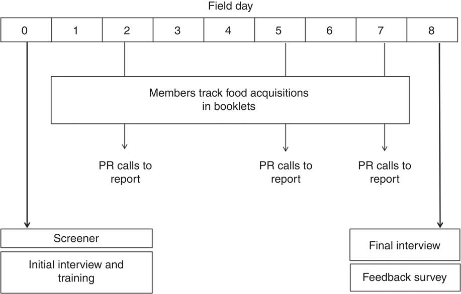
Fig. 1 Overview of the planned data collection week of FoodAPS (PR, primary respondent; FoodAPS, National Household Food Acquisition and Purchase Survey)
Table 1 Summary of information collected at each interview in FoodAPS
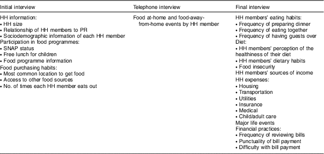
FoodAPS, National Household Food Acquisition and Purchase Survey; HH, household; PR, primary respondent; SNAP, Supplemental Nutrition Assistance Program.
Interviewers
Nearly 200 interviewers were hired to conduct the face-to-face interviews. The interviewers were provided with both an at-home training (where they had to track their own food acquisition for a week) and on-site training which lasted four or five days and covered: general training skills for inexperienced interviewers; specific training for screening households and conducting the initial and final interviews; and how to train respondents to use the food logs. At the end of the training, interviewers were evaluated on their knowledge and performance, and they were certified for data collection. Interviewers were assigned to geographical locations closest to their home. Every region was overseen by a field manager who monitored interviewer productivity in terms of response rates and contact rates. These data were not available for analysis.
Given the importance of average interviewer workload in determining the expected impacts of variable interviewer effects on the variance of survey estimates( Reference West and Blom 5 ), Table 2 summarizes the total number of interviewers (n) and their average workloads (i.e. counts of households or persons providing a value for that outcome) for each of the outcomes investigated in the present study. In Table 2, the average total workload for measures of food security, income and missing income are from the final interview, while SNAP discrepancy is from the initial interview. Interview day gap is based on the dates of the initial and final interviews, being constrained to households that had the same interviewer for both interviews. A total of 165 interviewers conducted the initial and final interviews for the same household. The workload reflects the number of initial and final interview pairs conducted on the same household. The individual income and missing income workloads are based on individual respondents rather than households, as the PR was asked about the income of each person aged 16 years or older within the household.
Table 2 Counts of interviewers and average workloads by outcome in FoodAPS
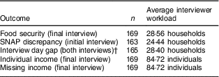
FoodAPS, National Household Food Acquisition and Purchase Survey; SNAP, Supplemental Nutrition Assistance Program.
† Measured only for households in which the same interviewer conducted both the initial and final interviews.
Outcome variables
As mentioned previously, five different survey outcomes were examined in the present study. Each outcome is described below, after restricting the sample to only those who have complete records on all the covariates of interest (detailed in the next section).
Food insecurity
Food insecurity, measured from the ten-item, 30 d USDA Food Security Module for adults, was collected at the final interview at the household level( 20 ). The sum of the scores for the scale ranges from 0 (no food insecurity) to 10 (highest food insecurity). In the present study, scores of 0–2 and 3–10 were collapsed into two separate categories, yielding a binary food security measure ‘food security’ v. ‘food insecurity’, as per USDA definitions( 17 ).
SNAP discrepancy
SNAP discrepancy was measured by matching household-level self-reports of current SNAP status collected at the initial interview against administrative records of their SNAP status. Prior consent to match their responses was obtained in the FoodAPS interview. Observations were coded as ‘discrepant’ when their reported SNAP status did not match administrative records.
Interview day gap
Although the planned data collection period spanned eight days, this was not always the case for a given household. The range of the data collection period spanned from 6 to 167 d, with an average of 9·8 d and a median of 8·0 d. Due to the skewed distribution, with a high number of interviews finishing on time (i.e. within 6–8 d), we grouped the raw measure into three ordinal categories (on time, 6–8 d; delayed, 9–10 d; extremely delayed, >10 d).
Total individual income
An individual’s monthly income was constructed from separate questions in the final interview about six different types of income for each household member who was at least 16 years old. In the final FoodAPS data set, any missing income at the individual level was imputed. As the interest in the present study was in interviewer effects on the measurement variance of this outcome, total individual income prior to imputation was used, and the analysis was restricted to individuals who reported any income at all, leaving 6753 observations for analysis.
Missing income
This variable was constructed from the total individual income variable. Observations that were flagged as having any imputed income amount (i.e. any item-missing on the six types of income) were coded as missing income, while all other observations were coded as non-missing.
Covariates
A total of eighteen household-level covariates, eight individual-level covariates and three interviewer-level covariates (see Tables 3 and 4) that might be associated with the five outcomes were identified from the FoodAPS data set and Census 2010 data. Covariates that were used in outcome variable construction, such as current SNAP status for the SNAP discrepancy outcome variable, were not included in the respective models. Food insecurity was dropped as a covariate for the food insecurity model. Employment status of the PR was dropped for the income and missing income models. In the model for income, household income was dropped as well. In the model for interview day gap, where the sample was restricted to households who were interviewed by the same interviewer at the initial and final interview, the interviewer familiarity covariate was dropped. Individual covariates were included only in the income and the missing income models.
Table 3 Household-level/individual-level covariates from FoodAPS included in the models
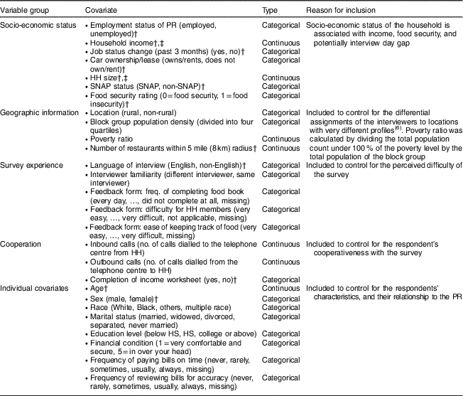
FoodAPS, National Household Food Acquisition and Purchase Survey; PR, primary respondent; HH, household; SNAP, Supplementary Nutrition Assistance Program; freq., frequency; HS, high school.
† Tested as random slopes, all not significant at α=0·05.
‡ Income was rescaled by 10 000; income and household size were mean-centred (i.e. the overall mean of the variable was subtracted from each individual value).
Table 4 Interviewer-level covariates from FoodAPS included in the models
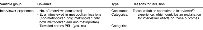
FoodAPS, National Household Food Acquisition and Purchase Survey; PSU, primary sampling unit.
† Number of interviews was mean-centred.
Statistical analysis
To examine interviewer effects on the five outcomes of interest, we fit separate generalized linear mixed models to each of the outcomes using PROC GLIMMIX in the statistical software package SAS version 9.4. We used a cumulative logit link for the interview day gap outcome (modelling the probability of a longer day gap), and a binary logit link for food insecurity (predicting the event of food insecurity), SNAP discrepancy (predicting the event of having a discrepancy) and missing income outcomes (predicting the event of missing income). We assumed that the income outcome followed a marginal normal distribution and employed an identity link for that model.
For each of these outcomes, we fit an unconditional model first, with a fixed overall intercept, a random interviewer effect (assumed to be normally distributed with a mean of 0 and constant variance) and a residual (for income, normally distributed with a mean of 0 and constant variance). In the individual models, a random household effect was added as well to account for the clustering within households. Our objective in fitting the initial unconditional model was to obtain an estimate of the raw between-interviewer variance in the random interviewer effects, prior to adjustment for the fixed effects of any covariates.
Following that, we fit a model including fixed effects of the household-level covariates to examine the change in interviewer variance after accounting for the possible household-level correlates of the outcomes. If a given interviewer worked on very similar households, these covariates may behave like interviewer-level covariates (having minimal variation within interviewers) and their subsequent fixed effects may then explain interviewer variance. Finally, we added the fixed effects of interviewer-level covariates to the model, again to examine the change in the interviewer variance after accounting for possible interviewer-level correlates of the outcomes. Because all models used the exact same cases with non-missing values on all variables (given the restrictions noted above), the interviewer variance was consistently estimated using the same cases across all steps. The variance components were tested for significant differences from zero using likelihood ratio tests based on mixtures of χ 2 probabilities( Reference West, Welch and Galecki 21 ).
The food insecurity and interview day gap models were estimated using the adaptive Gaussian quadrature (AGQ) method with ten integration points, while the individual income model was estimated using Laplace approximation, and the SNAP discrepancy and missing income models were estimated using the less computationally intensive (and potentially more biased) residual pseudo-likelihood estimation technique( Reference Kim, Choi and Emery 11 ). Given the relatively rare occurrence of SNAP discrepancies and the computational difficulty in fitting both a household and interviewer random intercept on a binary outcome, this approach was mainly used to get an approximate sense of any interviewer variance; the small prevalence prevented the AGQ from converging and producing a valid solution.
The possibility that the effects of particular covariates varied across interviewers was also tested in a purely exploratory fashion for all models (i.e. we did not have any theoretical expectations about particular relationships of the covariates with the outcomes that may vary across interviewers). The covariates for which we tested the possibility of random slopes are indicated in Table 2. The estimates given herein are all unweighted.
For each of these models, observations that were missing on any of the covariates were dropped from analysis. At each model-fitting step, an intraclass correlation coefficient (ICC) was calculated to determine how much of the total variance in a given outcome was accounted for by the interviewers. A high ICC would indicate that the interviewers were contributing substantially to the overall variance; the values observed in typical survey practice range between 0·01 (very small) to 0·12 or more (very large)( Reference West and Olson 12 ). The ICC was calculated with the following formula:
 $${\rm ICC}{\equals}{{\sigma _{0}^{2} } \over {\sigma _{0}^{2} {\plus}\sigma ^{2} }},$$
where $\sigma _{0}^{2} $
is the variance of the random interviewer effects and σ
2 is the unexplained residual variance within interviewers (fixed to π
2/3, or the fixed variance of the logistic distribution, for the logistic models). In the case of the income models, the ICC was calculated with the following formula, where the only addition is the variance of the random household effect denoted by
$\sigma _{0}^{2} $
is the variance of the random interviewer effects and σ
2 is the unexplained residual variance within interviewers (fixed to π
2/3, or the fixed variance of the logistic distribution, for the logistic models). In the case of the income models, the ICC was calculated with the following formula, where the only addition is the variance of the random household effect denoted by $\sigma _{{0,\,{\rm HH}}}^{2} $
:
$\sigma _{{0,\,{\rm HH}}}^{2} $
:
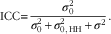 $${\mathop{\rm ICC}\nolimits} {\equals}{{\sigma _{0}^{2} } \over {\sigma _{0}^{2} {\plus}\sigma _{{0,\,{\mathop{\rm HH}\nolimits} }}^{2} {\plus}\sigma ^{2} }}.$$
After fitting the model that included the fixed effects of the household- (or individual-) and interviewer-level covariates, empirical best linear unbiased predictors (EBLUP) of the random interviewer effects in the model were computed and examined graphically. We first identified potential outliers in the distribution of the predicted random interviewer effects. We then profiled those interviewers found to be highly unusual and who could be influencing our estimates of the interviewer variance. Finally, the interviewer variance components were estimated again after excluding these potential outliers. Although there are other methods to identify outliers, such as using the random effects variance shift outlier model (RVSOM), which was developed for linear mixed models and is computationally more intensive, we opted for a graphical method as our outcomes are mostly categorical( Reference Gumedze and Jackson 22 ).
The multiplicative interviewer effect on the variance of a descriptive estimate( Reference West and Blom 5 ) was then calculated from the ICC after removal of the outliers, using the following formula:
 $${\rm Interviewer}\,{\rm effect}\,{\equals}\,1{\plus}(\bar{b}{\minus}1){\times}{\rm ICC,}$$
where $\bar{b}$
is the average interviewer workload for that outcome. For example, if the average interviewer workload
$\bar{b}$
is the average interviewer workload for that outcome. For example, if the average interviewer workload $\bar{b}$
is thirty interviews and the ICC is 0·10, there will be an almost 300 % increase in variance of a descriptive estimate (e.g. an estimated proportion) due to interviewer effects.
$\bar{b}$
is thirty interviews and the ICC is 0·10, there will be an almost 300 % increase in variance of a descriptive estimate (e.g. an estimated proportion) due to interviewer effects.
Results
Descriptive statistics
For those households with complete data on the covariates of interest, 72·15 % reported having ‘food security’, while the remaining 27·85 % reported having ‘food insecurity’. Out of the 94·05 % of households that provided match consent, only 3·48 % of the households had a discrepant report of their current SNAP status. As for interview day gap, 57·9 % of the final interviews were completed on time, 24·1 % were delayed and the remaining 18·1 % were extremely delayed. The range of total individual monthly income (in US dollars) was $4·17 to more than $90 000, with a median of $1660·00, a mean of $2329·34 and sd of $2846·55. Due to the skewed distribution of the responses, individual income was log-transformed for analysis. Of the 10 182 individuals who were 16 years or older, 13·83 % had missing income data.
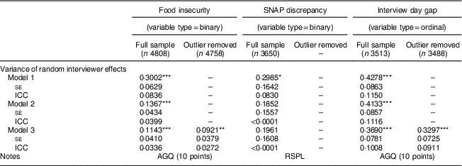
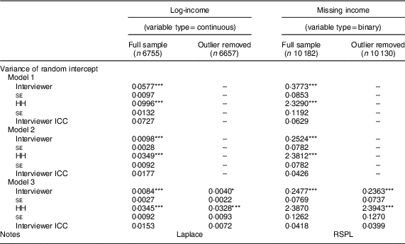
Interviewer effects
Due to very small cell sizes which led to the food insecurity model not converging, location of household, employment status of PR and household income were dropped as covariates in this model. Table 5 provides a summary of the estimated variances of the random interviewer effects in each of the models considered for the household-level outcomes (i.e. food insecurity, SNAP discrepancy, interview day gap), while Table 6 provides estimated variance components for the individual-level outcomes (i.e. income and missing income). For the outcomes, there is evidence of significant variation in the random interviewer effects in the unconditional model (Model 1), with the variability accounted for by the interviewers ranging from 8·30 % (SNAP discrepancy in Table 5) to 11·50 % (interview day gap in Table 5).
Table 5 Interviewer effects on the household-level outcomes in FoodAPS, with standard errors
FoodAPS, National Household Food Acquisition and Purchase Survey; SNAP, Supplementary Nutrition Assistance Program; ICC, intraclass correlation coefficient (for ordinal and binary outcomes, calculated using ICC= $\sigma _{\tf="Helvitica_font_roman" 0}^{\tf="Helvitica_font_roman" 2} {\rm /}\left( {\sigma _ {\tf="Helvitica_font_roman" 0}^{\tf="Helvitica_font_roman" 2} {\plus} {\tf="Helvitica_font_roman" 3\, \!\!\cdot\!\! 29}} \right)$
); AGQ, adaptive Gaussian quadrature; RSPL, restricted pseudo likelihood, Newton–Raphson optimization; HH, household.
$\sigma _{\tf="Helvitica_font_roman" 0}^{\tf="Helvitica_font_roman" 2} {\rm /}\left( {\sigma _ {\tf="Helvitica_font_roman" 0}^{\tf="Helvitica_font_roman" 2} {\plus} {\tf="Helvitica_font_roman" 3\, \!\!\cdot\!\! 29}} \right)$
); AGQ, adaptive Gaussian quadrature; RSPL, restricted pseudo likelihood, Newton–Raphson optimization; HH, household.
Model 1, unconditional model; Model 2, model with HH covariates; Model 3, model with HH and interviewer covariates; Model 3 outlier removed, model with HH and interviewer covariates (outlier interviewer removed).
Tested with mixture χ 2 test, first fitting the model with random household intercept, then the model with interviewer and household random intercepts; none of the models tested had evidence of random slopes. Rescaling of the interviewer variance component across the binary logit and cumulative logit models, given the household- and individual-level covariates included in Model 2, did not yield substantially different findings(24).
*P<0·05, **P<0·01, ***P<0·0001.
Table 6 Interviewer effects on the individual-level outcomes in FoodAPS, with standard errors
FoodAPS, National Household Food Acquisition and Purchase Survey; HH, household; ICC, intraclass correlation coefficient (for binary outcome, calculated using ICC= $\sigma _{\tf="Helvitica_font_roman" 0}^{\tf="Helvitica_font_roman" 2} {\rm /}\left( {\sigma _{\tf="Helvitica_font_roman" 0}^{\tf="Helvitica_font_roman" 2} {\plus}\sigma _{{{\mathop{\rm \tf="Helvitica_font_roman" HH}\nolimits} }}^{\tf="Helvitica_font_roman" 2} {\plus}\tf="Helvitica_font_roman" 3 \!\cdot\! 29} \right)$
); RSPL, restricted pseudo likelihood, Newton–Raphson optimization.
$\sigma _{\tf="Helvitica_font_roman" 0}^{\tf="Helvitica_font_roman" 2} {\rm /}\left( {\sigma _{\tf="Helvitica_font_roman" 0}^{\tf="Helvitica_font_roman" 2} {\plus}\sigma _{{{\mathop{\rm \tf="Helvitica_font_roman" HH}\nolimits} }}^{\tf="Helvitica_font_roman" 2} {\plus}\tf="Helvitica_font_roman" 3 \!\cdot\! 29} \right)$
); RSPL, restricted pseudo likelihood, Newton–Raphson optimization.
Model 1, unconditional model; Model 2, model with HH covariates; Model 3, model with HH and interviewer covariates; Model 3 outlier removed, model with HH and interviewer covariates (outlier interviewer removed).
Tested with mixture χ 2 test, first fitting the model with random household intercept, then the model with interviewer and household random intercepts; none of the models tested had evidence of random slopes. Rescaling of the interviewer variance component across the binary logit and cumulative logit models, given the household- and individual-level covariates included in Model 2, did not yield substantially different findings( Reference Hox, Moerbeek and van de Schoot 24 ).
*P<0·05, **P<0·01, ***P<0·0001.
The addition of fixed effects of the household-level covariates (i.e. Model 2) reduced the variance of the random interviewer effects for each of the five outcomes, as expected, but this reduction varied substantially in magnitude across the outcomes. For food insecurity and log-income, the variance of the random interviewer effects dropped by 54·46 % (equating to a change in the ICC from 0·0836 to 0·0399) and 83·02 % (ICC=0·0727 to 0·0177), respectively, while for the interview day gap and missing income outcomes the reduction was less pronounced. The estimated variance dropped by 3·39 % for interviewer day gap and 33·10 % for missing income. For the SNAP discrepancy model, adding the household-level covariates dropped the variance by 37·96 % (ICC=0·0830 to <0·0001) and the variance component was no longer significantly different from zero. Despite these reductions due to the addition of the household-level (and individual-level) covariates, there was still a significant amount of unexplained variance among the interviewers for four of the five models.
The addition of the fixed effects of the interviewer-level covariates (i.e. Model 3) did not change the variance of the random interviewer effects substantially in the missing income model; the variances of the random interviewer effects dropped by 1·86 %. The decreases in the variances of the random interviewer effects for the food insecurity model, interview day gap model and the income model were more substantial (i.e. 16·39 % in the food insecurity model, 10·72 % in the interview day gap model and 14·29 % in the log-income model).
Overall, the biggest drop in the variance for most of the models occurred after the inclusion of the fixed effects of the household-level covariates, suggesting that household-level features and the types of households recruited by the interviewers were playing a larger role in introducing variance in the outcomes among interviewers compared with interviewer-level covariates. However, neither the household-level covariates nor the interviewer-level covariates did well in reducing the variance of the random interviewer effects for the interview day gap model.
Examination of the empirical best linear unbiased predictors to identify outliers
Examination of the EBLUP of the random interviewer effects indicated that there were outliers in each of these models, except for SNAP discrepancy. From the four Q–Q plots of the EBLUP estimates (Fig. 2), we visually identified the most severe outlier for each outcome (circled on the plots). For illustration purposes, only one outlier has been selected for examination from the food insecurity model as it is less clear compared with the rest which is the most severe. We then examined these outliers based on covariates that are influential to the outcome (refer to Tables 7 and 8; covariates suppressed in the tables can be found in the online supplementary material, Supplemental Tables 1 to 4).
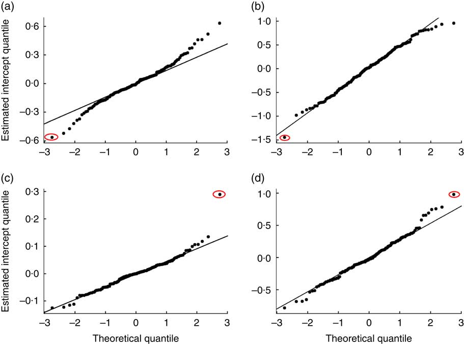
Fig. 2 (colour online) Q–Q plots of empirical best linear unbiased predictor estimates of the random interviewer effects in FoodAPS for: (a) food insecurity; (b) interview day gap; (c) income; (d) missing income. The most severe outlier for each outcome is circled (FoodAPS, National Household Food Acquisition and Purchase Survey)
Table 7 Odds ratios and 95 % confidence intervals for models with household and interviewer covariates (household models)Footnote †
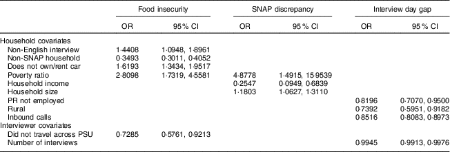
SNAP, Supplementary Nutrition Assistance Program; PR, primary respondent; primary sampling unit.
† Only covariates significant at P<0·01 are shown. Significance was tested with Wald test based on all parameters associated with the covariate.
Table 8 Estimates/odds ratios and 95 % confidence intervals for models with household and interviewer covariates (individual models)Footnote †
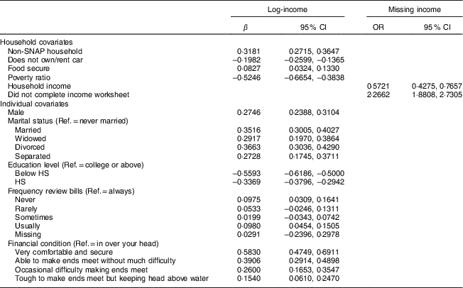
SNAP, Supplementary Nutrition Assistance Program; Ref., reference category; HS, high school.
† Only covariates significant at P<0·01 are shown. Significance was tested with Wald test based on all parameters associated with the covariate.
When the single outlier in the food insecurity model (Fig. 2(a)) was examined, we found that the households worked by this interviewer reported less food insecurity than expected (more seem to be food secure). Language of interview was a significant predictor of food insecurity, with non-English interviews being more likely to report food insecurity (OR=1·4408, 95 % CI 1·0948, 1·8961; Table 7). This interviewer conducted non-English interviews in twenty-one households but only one of them reported food insecurity, which was unusual. Compared with the whole sample, about 40 % of households with non-English interviews reported food insecurity.
The interviewer identified for the interview day gap model (Fig. 2(b)) was unusual because this interviewer did better than expected. This interviewer completed the final interview within the 8 d timeline for all twenty-five households assigned, despite half of the interviewed households having an employed PR. Based on the interview day gap model, PR who are not employed are less likely to take longer (OR=0·8196, 95 % CI 0·7070, 0·9500; which means PR who are employed are more likely to take longer).
The outlier interviewer for the log-income model (Fig. 2(c)) was unusual in that total incomes reported by most individuals in this interviewer’s households were roughly double their predicted income values based on the model. This interviewer was working primarily in rural areas with low poverty (100 % poverty rate of 0·005 to about 0·088 across the block groups worked). As can be seen in Fig. 3, three other interviewers who interviewed in areas with the same profile (Fig. 3(b), 3(c) and 3(d)) have a lower discrepancy between actual and predicted income. When the data from the outlier interviewer (Fig. 3(a)) were examined more closely, most respondents were recorded as receiving their reported earnings twice per month, which were then doubled during data processing to estimate the earnings portion of total monthly income. This pattern deviated from the majority of the sample, which indicated receiving their reported earnings once per month.
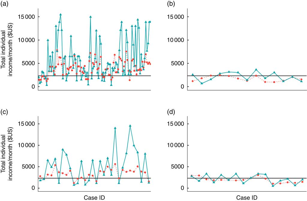
Fig. 3 (colour online) Predicted (![]() ) v. actual (
) v. actual (![]() ) individual income by interviewer in FoodAPS: (a) outlier: interviewer 490; (b) interviewer 469; (c) interviewer 531; (d) interviewer 663 (FoodAPS, National Household Food Acquisition and Purchase Survey)
) individual income by interviewer in FoodAPS: (a) outlier: interviewer 490; (b) interviewer 469; (c) interviewer 531; (d) interviewer 663 (FoodAPS, National Household Food Acquisition and Purchase Survey)
As for the missing income model (Fig. 2(d)), this interviewer was unusual because the degree of missingness for the income measure was higher than expected. In the full sample in this model, of those who completed the income worksheet prior to the final interview, only 9·50 % had any missing income measures at all. However, among those interviewed by this interviewer who had completed the income worksheet, 38·00 % of them had at least one missing income measure.
Even after removal of these outliers, a significant amount of interviewer variance remained (Tables 5 and 6). The income model saw a substantial change in the ICC (from ICC=0·0153 to 0·0072), or a 52·38 % reduction of the variance component of the interviewer after the removal of the outlier. The change was less dramatic in the other three models, with a 19·42 % reduction in the food insecurity model, a 10·65 % reduction in the interview day gap model and a 4·60 % reduction in the missing income model.
Multiplicative interviewer effects on variances of descriptive estimates
The ICC computed after the removal of the outliers were used in calculating the multiplicative interviewer effects for descriptive estimates (i.e. proportion indicating any food insecurity and mean individual income). This was not done for interview day gap and missing income, as these were constructed variables that measure survey quality. For food insecurity (unweighted mean=0·2806, se
SRS=0·0065; descriptive statistics estimated after removal of outliers and assuming simple random sampling), where the average interviewer workload was $\bar{b}$
=28·56 (Table 1) and the ICC was estimated to be 0·0272 (without the outlier), the resulting multiplicative interviewer effect was 1·75. Computing the standard error that accounts for the variance inflation due to the interviewer effects gives: se
INT=
$\bar{b}$
=28·56 (Table 1) and the ICC was estimated to be 0·0272 (without the outlier), the resulting multiplicative interviewer effect was 1·75. Computing the standard error that accounts for the variance inflation due to the interviewer effects gives: se
INT=
 $$\sqrt {\left( {0 \! \cdot \!0065^{2} {\times}1\! \cdot \!75} \right)} {\equals}0 \!\cdot \!0086$$
.
$$\sqrt {\left( {0 \! \cdot \!0065^{2} {\times}1\! \cdot \!75} \right)} {\equals}0 \!\cdot \!0086$$
.
Similarly, for individual income (unweighted mean=2277·38, se SRS=34·19), the interviewer effect was calculated to be 1·60 and, using the same equation as above, the standard error accounting for interviewer effects was 43·25 (a roughly 26 % increase). To illustrate the improvement in the estimates by removing the outlier, the estimated standard error accounting for interviewer effects prior to the removal of outliers for food insecurity is 0·0090 (interviewer effect=1·93, unweighted mean=0·2785, se SRS=0·0065). The standard error estimate of 0·0086 after removal of the outliers is only a minor improvement (4·44 %) over 0·0090.
It should be noted that although the ICC ranged from 0·0072 (very small) to 0·0911 (large) after the removal of the outlier interviewers, overall multiplicative interviewer effects on the variances of estimates are a function of both the ICC and interviewer workload. With an ICC of 0·0072, if the average interviewer workload is 100 instead, the interviewer effect would have been 1·70 instead of 1·60 and the standard error accounting for interviewer effects would have increased by 31 %. Therefore, even a small ICC may be cause for concern, depending on the average interviewer workload.
Discussion
The current study presented evidence of significant unexplained variance among FoodAPS interviewers in terms of reported values for interview day gaps and presence of missing income values, even after accounting for a variety of household- and interviewer-level covariates. Levels of unexplained variance among interviewers for measures of any food insecurity and total income were much lower. We conclude that some interviewer effects are indeed present in FoodAPS, and this raises concerns about the need to deal with interviewer effects in food acquisition surveys more generally for both data users and data producers( Reference Turrell, Hewitt and Patterson 15 , Reference Turrell and Kavanagh 16 ). Different interviewers were somehow eliciting different responses (or responses of varying quality) from respondents despite efforts to standardize their training. A failure of the secondary analyst to account for these interviewer effects in their substantive models may lead to overly liberal conclusions (i.e. increased type I error rate) and understated standard errors of key estimates as interviewer effects would inflate standard errors. It is also possible that different interviewers were successfully recruiting and interviewing different types of respondents, which could lead to different responses being elicited as well( Reference O’Muircheartaigh and Campanelli 7 , Reference Korbmacher and Schroeder 8 , Reference West and Olson 12 , Reference West, Kreuter and Jaenichen 23 ). As there was a lack of data on interviewer characteristics available from the FoodAPS, it is not possible with the current data set to determine if interviewers were in fact recruiting respondents more similar to themselves, as has been found in previous research( Reference West and Blom 5 , Reference West and Olson 12 ).
In practice, this problem could be reduced by having more standardization in the interviewing protocol, more rigorous interviewer training and, most importantly, field monitoring of large deviations from the patterns of the data collected. In the case of the possibility that interviewers were recruiting different types of respondents, efforts could be made to monitor the profiles of respondents recruited by each interviewer and intervene if the respondent profiles lack diversity. However, monitoring interviewer-level deviations from the pattern of responses collected may be slightly challenging; using multilevel modelling for such ‘live’ monitoring has not been done during survey operations before, to the authors’ knowledge. The effectiveness of this type of monitoring for interviewer effects during a data collection period requires future research.
In the analysis presented above, the current paper attempted to identify interviewers who may be contributing heavily to the interviewer effects. We were able to identify outliers for four of the models investigated. Removal of interviewers that were found to be outliers helped to reduce the variance for the individual income model, but not substantially for the other models. We also profiled these interviewers and tried to determine why their data were unusual.
This work therefore provides preliminary evidence of the efficacy of using multilevel modelling techniques to monitor interviewers in the field during data collection. By being able to monitor in real time, errors in data collection could be reduced. This approach does need some empirical backing before it could be implemented, so this monitoring could be started a few weeks into the data collection period or after some agreed-upon data collection threshold. RVSOM could also be implemented to identify influential outliers where possible to make outlier monitoring less subjective to human judgement( Reference Gumedze and Jackson 22 ).
Limitations
The main limitation for many studies on interviewer effects is the lack of randomization of interviewers to respondents, and this is true for the present study as well. To keep costs low, FoodAPS interviewers tended to be assigned to a few locations that were near their homes to reduce travel time and costs. The infeasibility of such a design means that interviewer effects may be confounded with geographical effects( Reference O’Muircheartaigh and Campanelli 7 ). The current paper tries to address this problem by including geographic information as covariates, but there could be geographic information that was not accounted for. Given this limitation, if important geographic covariates have been omitted from the models (which simply were not available in the data set), the effects of these covariates on the outcomes would be attributed to the interviewers. If a given interviewer also tended to work households with very similar characteristics, those household characteristics could also be driving the unexplained interviewer variance. We made a distinct effort to account for as many relevant household covariates as we could in the models fitted (Table 2).
The current data set also lacks information on the interviewers themselves, which is another major limitation; interviewer characteristics could be a factor in the responses they receive( Reference West and Blom 5 ). It would have been ideal to be able to include interviewer characteristics such as interviewer experience, race, age and gender, but the FoodAPS contractor did not provide any information about its interviewers. The present study attempted to include variables that could indicate interviewer experience (e.g. greater caseload could indicate a more experienced interviewer; refer to Table 4 for proxy covariates included). As with the geographical information, these models could have been improved by having more information on the interviewers.
More generally, we analysed only five outcome measures that we deemed likely to be prone to interviewer effects and/or important for a wide variety of users of FoodAPS data (e.g. any food insecurity). There may be interviewer effects on other FoodAPS measures as well.
Conclusion
Despite these limitations, the fact that a multilevel modelling approach was able to identify unusual interviewers lends credibility to our suggested approach of ‘live’ field monitoring. With a well-specified model for important outcomes and survey quality measures, this approach could potentially identify interviewers who may be performing differently, leading to recommendations for retraining. Ultimately, this could reduce interviewer effects for the outcomes that are important to a given survey, which in the case of FoodAPS would be any food insecurity and other variables related to food acquisition.
Acknowledgements
Financial support: This research was supported by a cooperative assistance grant (59-5000-5-0008) from the Economic Research Service of the US Department of Agriculture. The views expressed are those of the authors and should not be attributed to the Economic Research Service or the US Department of Agriculture. Conflict of interest: None. Authorship: A.R.O. and M.H. performed data analysis with advisement from B.T.W. Data access was provided by J.A.K. All authors contributed to the design of the study and to drafting and revising the manuscript. Ethics of human subject participation: FoodAPS was approved by the survey contractor’s (Mathematica Policy Research) institutional review board and the Office of Management and Budget.
Supplementary material
To view supplementary material for this article, please visit https://doi.org/10.1017/S1368980018000137


