


1. Introduction and main results
In this paper, we consider the existence of positive solutions to the following Kirchhoff-type problem:
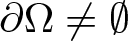
 \begin{equation}
\left\{
\begin{array}{ll}
-\left(a+b\displaystyle{\int}_{\Omega}|\nabla u|^{2}\,{\rm d}x\right)\triangle u+\lambda u=f(u), & x\in\Omega,\\
\\
u=0,& x\in\partial \Omega,\\
\end{array}\right.
\end{equation}
\begin{equation}
\left\{
\begin{array}{ll}
-\left(a+b\displaystyle{\int}_{\Omega}|\nabla u|^{2}\,{\rm d}x\right)\triangle u+\lambda u=f(u), & x\in\Omega,\\
\\
u=0,& x\in\partial \Omega,\\
\end{array}\right.
\end{equation}where a > 0,  $b\geq0$, and λ > 0 are constants, $\Omega\subset\mathbb{R}^{3}$ is an unbounded exterior domain, $\partial\Omega\neq\emptyset$, $\mathbb{R}^{3}\backslash\Omega$ is bounded, and $f\in C^1(\mathbb{R},\mathbb{R})$ that satisfies some conditions, which will be stated later on.
This type problem is called a non-local problem because of the presence of  $\int_{\Omega}|\nabla u|^{2}\,{\rm d}x$, which implies that Equation (1.1) is not a pointwise identity. This phenomenon causes some mathematical difficulties which make the study of such a class of problems particularly interesting. If $\Omega=\mathbb R^3$, then the rescaling
 \begin{equation*}
v(x)=u(\varpi_ux), \qquad \varpi_u=a+b\int_{\mathbb R^3}|\nabla u|^2\,{\rm d}x
\end{equation*}
\begin{equation*}
v(x)=u(\varpi_ux), \qquad \varpi_u=a+b\int_{\mathbb R^3}|\nabla u|^2\,{\rm d}x
\end{equation*}reduces the problem (1.4) into a local problem
 \begin{equation*}
-\Delta v+\lambda v=f(v), \qquad x\in \mathbb R^3.
\end{equation*}
\begin{equation*}
-\Delta v+\lambda v=f(v), \qquad x\in \mathbb R^3.
\end{equation*} However, under our assumption,  $\Omega\neq\mathbb R^3$; therefore, this reduction does not work any more.
A prototype of problem (1.1) arises from the following time-dependent wave equation proposed by Kirchhoff (see [Reference Kirchhoff15]) in 1883:
 \begin{equation*}
\rho\,\frac{\partial^{2}u}{\partial t^{2}}-\left(\frac{P_{0}}{h}+\frac{E}{2L}\int_{0}^{L}\left|\frac{\partial u}{\partial x}\right|^{2}\right)\frac{\partial^{2}u}{\partial x^{2}}=0,
\end{equation*}
\begin{equation*}
\rho\,\frac{\partial^{2}u}{\partial t^{2}}-\left(\frac{P_{0}}{h}+\frac{E}{2L}\int_{0}^{L}\left|\frac{\partial u}{\partial x}\right|^{2}\right)\frac{\partial^{2}u}{\partial x^{2}}=0,
\end{equation*}which is an extension of the classical d’Alembert wave equation for free vibration of elastic strings. Kirchhoff model takes into account the changes in the length of the string produced by transverse vibrations. Some early classical investigations of this model can be seen in Bernstein [Reference Bernstein5] and Pohoẑaev [Reference Pohozaev27]. However, only after the pioneer work of Lions [Reference Lions19], where a functional analysis approach was proposed, the Kirchhoff-type equations began to call more attention of researchers, see [Reference Arosio and Panizzi2, Reference Cavalcanti, Cavalcanti and Soriano7, Reference D’Ancona and Spagnolo9] and the references therein.
In recent years, Kirchhoff problems have been extensively studied by using variational methods, mainly in bounded domain or in whole space  $\mathbb{R}^{N}$. For bounded domain case, a number of results have been established (see, e.g., [Reference Alves, Correa and Ma1, Reference Bensedki and Bouchekif4, Reference Chen, Kuo and Wu8, Reference He and Zou12, Reference Mao and Zhang23, Reference Yang and Zhang35, Reference Zhang and Perera37] and the subsequent references). However, such problems become more complicated in $\mathbb{R}^{N}$ since the Sobolev embedding is not compact. Then it is hard to prove the strong convergence of a minimizing sequence or a Palais–Smale sequence, which makes the problems more attractive. So a considerable effort has been devoted by many researcher in the whole space. We only focus on the type of Kirchhoff equations similar to Equation (1.1) now, namely,
 \begin{equation}
\left\{
\begin{array}{ll}
-\left(a+b\displaystyle{\int}_{\mathbb{R}^{N}}|\nabla u|^{2}\,{\rm d}x\right)\triangle u+V(x)u=f(u), & x\in \mathbb{R}^{N},\\
\\
u\in H^{1}(\mathbb{R}^{N}),\\
\end{array}\right.
\end{equation}
\begin{equation}
\left\{
\begin{array}{ll}
-\left(a+b\displaystyle{\int}_{\mathbb{R}^{N}}|\nabla u|^{2}\,{\rm d}x\right)\triangle u+V(x)u=f(u), & x\in \mathbb{R}^{N},\\
\\
u\in H^{1}(\mathbb{R}^{N}),\\
\end{array}\right.
\end{equation}and its variants, where  $V\in C(\mathbb{R}^{N},\mathbb{R})$, $N\geq1$, a > 0 and $b\geq0$ are constants, and $f\in C(\mathbb{R},\mathbb{R})$ is subcritical and superlinear near infinity (see, e.g., [Reference Guo11, Reference He and Zou13, Reference Li, Luo, Peng, Wang and Xiang17, Reference Li and Ye18, Reference Liu, Liao and Pan20–Reference Lu and Lu22, Reference Sun and Zhang30, Reference Sun and Zhang31, Reference Wu, Zhou and Gu33, Reference Xie and Ma34, Reference Zhang and Du36]); one usually assumes that $V(x)\equiv1$, or V(x) is periodic, or $V(x)=V(|x|)$, or V(x) is coercive.
Particularly, the existence of solutions to Equation (1.2) and its variants was usually obtained by looking for the so-called ground states (see [Reference Guo11, Reference He and Zou13, Reference Li, Luo, Peng, Wang and Xiang17, Reference Li and Ye18, Reference Liu, Liao and Pan20–Reference Lu and Lu22, Reference Sun and Zhang30, Reference Sun and Zhang31], etc). As we know, minimizing technique and the Mountain Pass Lemma are typical ways to deal with this problem. For the special case  $f(u)=|u|^{p-2}u$, we refer readers to see [Reference Li, Luo, Peng, Wang and Xiang17, Reference Li and Ye18, Reference Lu and Lu22, Reference Sun and Zhang30, Reference Sun and Zhang31]. Sun and Zhang [Reference Sun and Zhang30, Reference Sun and Zhang31] obtained the existence, uniqueness, and asymptotic behaviour of the positive ground state solutions for $p\in(4,6)$. In [Reference Li and Ye18], using the constrained minimization on a Nehari–Pohozaev manifold, Li and Ye proved the existence of positive least energy solutions for $p\in(3,6)$. More recently, [Reference Li, Luo, Peng, Wang and Xiang17, Reference Lu and Lu22] generalized these results for $p\in(2,6)$. For the general case of f which satisfies various conditions, He and Zou [Reference He and Zou13] studied the Kirchhoff problem with 4-superlinear nonlinearities, that is, f satisfies the Ambrosetti–Rabinowitz-type condition: there exists µ > 4 such that
 \begin{equation}
0\lt\mu F(s)\leq f(s)s,\qquad {\rm for} \ s\gt0.
\end{equation}
\begin{equation}
0\lt\mu F(s)\leq f(s)s,\qquad {\rm for} \ s\gt0.
\end{equation}In [Reference Guo11], Guo generalized the results in [Reference He and Zou13] by a new Nehari–Pohozaev manifold, while f may not be 4-superlinear at infinity. Later, using an abstract critical point theorem established by Jeanjean, authors of [Reference Liu, Liao and Pan20, Reference Liu and Guo21] showed the existence of positive ground-state solutions with Berestycki–Lions conditions, which improved the 4-superlinear conditions.
The aim of this paper is to study the existence of positive solutions for Equation (1.1) in exterior domain Ω, with superlinear nonlinearities. However, methods used in the above papers, especially minimizing technique, is not applicable for our problem. Because our exterior domain Ω is unbounded but not the whole space, which implies Equation (1.1) has no ground-state solution (see Lemma 2.3), we have to find other types of solutions in the absence of ground states, and this needs a deeper understanding of the obstructions to the compactness.
The motivation of the present paper comes from a paper due to Benci and Cerami [Reference Benci and Cerami3], in which the authors studied the existence of positive solutions to the problem
 \begin{equation}
-\Delta u+\lambda u=|u|^{q-2}u, \quad \text{in} \ \Omega,
\end{equation}
\begin{equation}
-\Delta u+\lambda u=|u|^{q-2}u, \quad \text{in} \ \Omega,
\end{equation}where λ > 0,  $2\lt q\lt6$, and $u\in H_{0}^{1}(\Omega)$ and $\Omega\subset\mathbb{R}^{N}$ ( $N\geq3$) is an exterior domain. In [Reference Benci and Cerami3], the authors used a constrained variational technique which depends on the homogeneity of the problem (1.4). In this paper, we consider problem with nonlocal term $\int_{\Omega}|\nabla u|^{2}\,{\rm d}x$ that destroys the homogeneity. Moreover, owing to the presence of the nonlocal term, one does also not permit to use the same method of paper [Reference Benci and Cerami3] directly in the verification of compactness for Palais–Smale sequence. So we must overcome some specific difficulties in different ways. We intend to show in the present paper how we can work with this nonlocal term to get a positive solution for Equation (1.1).
Our study is based on variational methods. The principle difficulties lie in the following aspects: (1) In this paper, we use a different constraint, the Nehari manifold constraint, to overcome the difficulty of nonhomogeneity. Accordingly, more delicate analysis is needed, see Lemmas 2.1, 2.3, and 3.2. (2) Because of complex geometry of  $\partial\Omega$, it is hard to use Pohozaev identity, which is commonly used in many papers to deal with the non-local term, we make our nonlinearity f to be 4-superlinear. (3) We would like to emphasize that one important difficulty of the present paper is the verification of compactness for Palais–Smale sequence, see Lemma 2.2 and the compactness Lemmas 3.1–3.3.
To our best knowledge, there has been no article yet that concerns the existence of positive solutions for Kirchhoff equations of type (1.1) and its similar variants in exterior domains; the existing researches of this problem are all settled in bounded domains or the whole space. In the present paper, we shall establish some existence results for positive solutions of Kirchhoff-type problem (1.1). Besides, we also generalize the results in [Reference Benci and Cerami3] for the Schrödinger equation (1.4).
Before stating the main results, we make the following assumptions: $(F_{1})$ $\lim_{s\rightarrow0}f(s)/s=0$, $\lim_{|s|\rightarrow+\infty}f(s)/s^{5}=0$. $(F_{2})$ $\lim_{|s|\rightarrow+\infty}F(s)/s^{4}=+\infty$, where $F(s)=\int_{0}^{s}f(t)\,{\rm d}t$. $(F_{3})$ $s\mapsto f(s)/s^{3}$ is positive for s ≠ 0, non-decreasing on $(0,+\infty)$. $(F_{4})$There exists a constant C > 0 such that
 \begin{equation*}
|f^\prime(s)|\leq C(|s|^{4}+1)\text{ for any } s\gt0.
\end{equation*}
\begin{equation*}
|f^\prime(s)|\leq C(|s|^{4}+1)\text{ for any } s\gt0.
\end{equation*}Our main results are as follows:
Theorem 1.1. Assume a > 0,  $b\geq0$, λ > 0, and $(F_{1})$– $(F_{4})$ hold. If the equation
 \begin{equation}
-\Delta u+\lambda u=f(u), \qquad u\in H^{1}(\mathbb{R}^{3})
\end{equation}
\begin{equation}
-\Delta u+\lambda u=f(u), \qquad u\in H^{1}(\mathbb{R}^{3})
\end{equation}has at most finite number of positive solutions, then there exists small  $\widetilde{\rho}:=\widetilde{\rho}(\lambda)$ such that if
 \begin{equation*}
{\rm diam}(\mathbb{R}^{3}\setminus\Omega):=\sup\{|x-y|: \ x,y\in \mathbb{R}^{3}\setminus\Omega\}\lt\widetilde{\rho},
\end{equation*}
\begin{equation*}
{\rm diam}(\mathbb{R}^{3}\setminus\Omega):=\sup\{|x-y|: \ x,y\in \mathbb{R}^{3}\setminus\Omega\}\lt\widetilde{\rho},
\end{equation*}the problem (1.1) has at least one positive solution.
Theorem 1.2. Assume a > 0,  $b\geq0$, and $(F_{1})$– $(F_{4})$ hold. Then there exists $\lambda_{\ast}:=\lambda_{\ast}(\Omega)\gt0$ such that for every $\lambda\in(0,\lambda_{\ast})$, if Equation (1.5) has at most finite number of positive solutions, then the problem (1.1) has at least one positive solution.
Remark 1.1. Many results concerning the uniqueness of positive solutions for Equation (1.5) have been obtained under various conditions; we refer the readers to see [Reference Kwong16, Reference Mcleod24–Reference Peletier and Serrin26, Reference Serrin and Tang29] and the references therein. For example, in 1993, Mcleod [Reference Mcleod24] proved that Equation (1.5) has a unique positive solution under assumption  $(F_{1})$ and the following two conditions: $(F_{5})$ $f\in C^1(\mathbb{R}, \mathbb{R})$, there exists α > 0 such that $f^\prime(\alpha)\gt\lambda\gt0$,
 \begin{equation*}
f(s)\lt\lambda s\ \text{for} \ 0 \lt s\lt\alpha, \qquad f(s)\gt\lambda s\
\text{for} \ s\gt\alpha,
\end{equation*}
\begin{equation*}
f(s)\lt\lambda s\ \text{for} \ 0 \lt s\lt\alpha, \qquad f(s)\gt\lambda s\
\text{for} \ s\gt\alpha,
\end{equation*}and there exists  $\beta\gt\alpha$ such that $F(\beta)=\frac{1}{2}\lambda\beta^{2}$, where $F(s)=\int_{0}^{s}f(t)\,{\rm d}t$. $(F_{6})$For τ > 0, we define
  $I(s,\tau)=\tau
sf^\prime(s)-(\tau+2)f(s)+2\lambda s$, then for each
$I(s,\tau)=\tau
sf^\prime(s)-(\tau+2)f(s)+2\lambda s$, then for each  $U\gt\alpha$, there is a $\tau(U)\gt0$ such that
 \begin{equation*}
I(s,\tau(U))\geq0\ \text{for} \ 0 \lt s \lt U, \qquad I(s,\tau(U))\leq0\
\text{for} \ s \gt U.
\end{equation*}
\begin{equation*}
I(s,\tau(U))\geq0\ \text{for} \ 0 \lt s \lt U, \qquad I(s,\tau(U))\leq0\
\text{for} \ s \gt U.
\end{equation*} It is not hard to see that  $(F_{3})$, $(F_{5})$, and $(F_{6})$ implies $(F_{4})$, and as a result, we obtain the following corollary.
Corollary 1.1. Assume a > 0,  $b\geq0$, λ > 0, $(F_{1})$– $(F_{3})$, and $(F_{5})$ and $(F_{6})$ hold. Then
(1) there exists small $\widetilde{\rho}:=\widetilde{\rho}(\lambda)$ such that if
the problem (1.1) has at least one positive solution;\begin{equation*}
{\rm diam}(\mathbb{R}^{3}\setminus\Omega)\lt\widetilde{\rho},\\[-6pt]
\end{equation*}
$\widetilde{\rho}:=\widetilde{\rho}(\lambda)$ such that if
the problem (1.1) has at least one positive solution;\begin{equation*}
{\rm diam}(\mathbb{R}^{3}\setminus\Omega)\lt\widetilde{\rho},\\[-6pt]
\end{equation*}(2) there exists
$\lambda_{\ast}:=\lambda_{\ast}(\Omega)\gt0$ such that if $\lambda\in(0,\lambda_{\ast})$, the problem (1.1) has at least one positive solution.


Example 1.1. Let  $p_{i}\in(4,6)$, $a_i\gt0$, $i=1,2,\ldots,n$, then for any λ > 0
 \begin{equation*}
f(s):=a_{1}|s|^{p_{1}-2}s+a_{2}|s|^{p_{2}-2}s+\cdots+a_{n}|s|^{p_{n}-2}s, \qquad s\in \mathbb{R}
\end{equation*}
\begin{equation*}
f(s):=a_{1}|s|^{p_{1}-2}s+a_{2}|s|^{p_{2}-2}s+\cdots+a_{n}|s|^{p_{n}-2}s, \qquad s\in \mathbb{R}
\end{equation*}satisfies  $(F_{1})$– $(F_{6})$.
Remark 1.2. When b = 0, then after a suitable scaling, Equation (1.1) reduces to the following Schrödinger equation with general nonlinearity
 \begin{equation}
-\Delta u+\lambda u=f(u), \qquad \text{in} \ \Omega.
\end{equation}
\begin{equation}
-\Delta u+\lambda u=f(u), \qquad \text{in} \ \Omega.
\end{equation} Assume that f satisfies assumptions  $(F_{1})$ and $(F_{4})$ and the following assumptions: $(F^\prime_{2})$ $\lim_{|s|\rightarrow+\infty}F(s)/s^{2}=+\infty$, where $F(s)=\int_{0}^{s}f(t)\,{\rm d}t$, $(F^\prime_{3})$ $s\mapsto f(s)/s$ is strictly increasing in $(0,+\infty)$.
By using the technique used in this paper, the following results can be obtained, which extend the results in [Reference Benci and Cerami3].
Corollary 1.2. Assume λ > 0 and  $(F_{1})$, $(F^\prime_{2})$, $(F^\prime_{3})$, and $(F_{4})$ hold. If Equation (1.5) has at most finite number of positive solutions, then
(1) there exists small
$\widetilde{\rho}:=\widetilde{\rho}(\lambda)$ such that if
the problem (1.6) has at least one positive solution;\begin{equation*}
{\rm diam}(\mathbb{R}^{3}\setminus\Omega)\lt\widetilde{\rho},\\[-6pt]
\end{equation*}(2) there exists
$\lambda_{\ast}:=\lambda_{\ast}(\Omega)\gt0$ such that if $\lambda\in(0,\lambda_{\ast})$, the problem (1.6) has at least one positive solution.


Corollary 1.3. Assume λ > 0 and  $(F_{1})$, $(F^\prime_{2})$, $(F^\prime_{3})$, $(F_{5})$, and $(F_{6})$ hold. Then
(1) there exists small
$\widetilde{\rho}:=\widetilde{\rho}(\lambda)$ such that if
the problem (1.6) has at least one positive solution;\begin{equation*}
{\rm diam}(\mathbb{R}^{3}\setminus\Omega)\lt\widetilde{\rho},
\end{equation*}(2) there exists
$\lambda_{\ast}:=\lambda_{\ast}(\Omega)\gt0$ such that if $\lambda\in(0,\lambda_{\ast})$, the problem (1.6) has at least one positive solution.


This paper is organized as follows. In  $\S$ 2, we establish the variational framework of Equation (1.1) and give some preliminary lemmas. In $\S$ 3, we give the compactness results which are necessary to prove our results. In $\S$ 4, we give the detailed proof of Theorems 1.1 and 1.2.
2. Preliminary lemmas
In this section, we give the variational setting and some notations for problem (1.1). We consider (1.1) in the space  $H^{1}_{0}(\Omega)$. It is well known that the solutions of (1.1) are the critical points of the energy functional $I: H_{0}^{1}(\Omega)\rightarrow\mathbb{R}$ defined by
 \begin{equation}
I(u):=\frac{1}{2}\int_{\Omega}\left(a\left|\nabla u\right|^{2}+\lambda
u^{2}\right)\,{\rm d}x+\frac{b}{4}\left(\int_{\Omega}|\nabla
u|^{2}\,{\rm d}x\right)^{2}-\int_{\Omega}F(u)\,{\rm d}x.
\end{equation}
\begin{equation}
I(u):=\frac{1}{2}\int_{\Omega}\left(a\left|\nabla u\right|^{2}+\lambda
u^{2}\right)\,{\rm d}x+\frac{b}{4}\left(\int_{\Omega}|\nabla
u|^{2}\,{\rm d}x\right)^{2}-\int_{\Omega}F(u)\,{\rm d}x.
\end{equation} We recall that for any smooth open domain  $D\subset\mathbb{R}^{3}$, $H^{1}_{0}(D)$ denote a Hilbert space obtained as closure of $C_{0}^{\infty}(D)$ under the inner product and norm, respectively,
 \begin{equation*}
(u,v)=\int_{D}\left(a\nabla u\nabla v+\lambda uv\right)\,{\rm d}x,\quad \|u\|^{2}=(u,u).
\end{equation*}
\begin{equation*}
(u,v)=\int_{D}\left(a\nabla u\nabla v+\lambda uv\right)\,{\rm d}x,\quad \|u\|^{2}=(u,u).
\end{equation*}  $H^{1}(\mathbb{R}^{3})$ is the usual Sobolev space endowed with the inner product and norm, respectively,
 \begin{equation*}
(u,v)_{\mathbb{R}^{3}}=\int_{\mathbb{R}^{3}}\left(a\nabla u\nabla v+\lambda uv\right)\,{\rm d}x,\quad \|u\|_{\mathbb{R}^{3}}^{2}=(u,u)_{\mathbb{R}^{3}}.
\end{equation*}
\begin{equation*}
(u,v)_{\mathbb{R}^{3}}=\int_{\mathbb{R}^{3}}\left(a\nabla u\nabla v+\lambda uv\right)\,{\rm d}x,\quad \|u\|_{\mathbb{R}^{3}}^{2}=(u,u)_{\mathbb{R}^{3}}.
\end{equation*}  $L^{q}(\mathbb{R}^{3})$ and $L^{q}(\Omega)$, $1\leq q\lt+\infty$, are the class of measurable functions u which satisfies $\int_{\mathbb{R}^{3}}|u|^{q}\,{\rm d}x\lt+\infty$ and $\int_{\Omega}|u|^{q}\,{\rm d}x\lt+\infty$, respectively, and we denote the norm of $L^{q}(\mathbb{R}^{3})$ and $L^{q}(\Omega)$ by
 \begin{equation*}
\left|u\right|_{L^{q}(\mathbb{R}^{3})}=\left(\int_{\mathbb{R}^{3}}|u|^{q}\,{\rm d}x\right)^{\frac{1}{q}},\qquad \left|u\right|_{q}=\left(\int_{\Omega}|u|^{q}\,{\rm d}x\right)^{\frac{1}{q}},
\end{equation*}
\begin{equation*}
\left|u\right|_{L^{q}(\mathbb{R}^{3})}=\left(\int_{\mathbb{R}^{3}}|u|^{q}\,{\rm d}x\right)^{\frac{1}{q}},\qquad \left|u\right|_{q}=\left(\int_{\Omega}|u|^{q}\,{\rm d}x\right)^{\frac{1}{q}},
\end{equation*}respectively. We define the Nehari manifold  $\mathcal{N}$ for functional I by
 \begin{equation*}
\mathcal{N}:=\{u\in H_{0}^{1}(\Omega)\backslash\{0\}:G(u)=0\}, \qquad
G(u):=\langle I^\prime(u),u\rangle,
\end{equation*}
\begin{equation*}
\mathcal{N}:=\{u\in H_{0}^{1}(\Omega)\backslash\{0\}:G(u)=0\}, \qquad
G(u):=\langle I^\prime(u),u\rangle,
\end{equation*}and we give the next lemma to state some properties of  $\mathcal{N}$.
Lemma 2.1. Let a > 0,  $b\geq0$, λ > 0, and $(F_{1})$– $(F_{3})$ hold. Then the following statements hold:
(1)
$\mathcal{N}$ is a C 1 regular manifold diffeomorphic to the unit sphere of $H^{1}_{0}(\Omega)$;(2) I is bounded from below on
$\mathcal{N}$ by a positive constant;(3) u is a critical point of I if and only if u is a critical point of I constrained on
$\mathcal{N}$.


Proof. (1) Let  $u\in H^{1}_{0}(\Omega)$ be such that $\|u\|=1$. We claim that there exists a unique $t\in (0,+\infty)$ such that $tu\in\mathcal{N}$. By $(F_{1})$, for any ɛ > 0 and $s\in \mathbb{R}$, there exists a constant $C(\varepsilon)\gt0$ such that
 \begin{equation}
|f(s)|\leq\varepsilon|s|+C(\varepsilon)|s|^{5}
\end{equation}
\begin{equation}
|f(s)|\leq\varepsilon|s|+C(\varepsilon)|s|^{5}
\end{equation}and
 \begin{equation}
|F(s)|\leq\frac{1}{2}\varepsilon|s|^{2}+\frac{1}{6}C(\varepsilon)|s|^{6}.
\end{equation}
\begin{equation}
|F(s)|\leq\frac{1}{2}\varepsilon|s|^{2}+\frac{1}{6}C(\varepsilon)|s|^{6}.
\end{equation} Set  $\alpha_{u}(t):=I(tu)$. Clearly, $\alpha_{u}(0)=0$ and $\alpha_{u}^\prime(0)=0$. For any fixed ɛ > 0, we have
 \begin{equation*}\begin{array}{rcl}
\alpha_{u}(t)&=&\displaystyle{\frac{1}{2}t^{2}\int_{\Omega}\left(a|\nabla u|^{2}+\lambda u^{2}\right)\,{\rm d}x+\frac{1}{4}bt^{4}\left(\int_{\Omega}|\nabla u|^{2}\,{\rm d}x\right)^{2}-\int_{\Omega}F(tu)\,{\rm d}x}\\
\\
&\geq&\displaystyle{\frac{1}{2}t^{2}\int_{\Omega}\left(a|\nabla u|^{2}+\lambda u^{2}\right)\,{\rm d}x+
\frac{1}{4}bt^{4}\left(\int_{\Omega}|\nabla u|^{2}\,{\rm d}x\right)^{2}}\\
\\
&\quad&\displaystyle{-\int_{\Omega}\left[\frac{1}{2}\varepsilon|tu|^{2}+\frac{1}{6}C(\varepsilon)|tu|^{6}\right]\,{\rm d}x \geq\displaystyle{\frac{1}{2}t^{2}-c_{1}\varepsilon
t^{2}-c_{2}C(\varepsilon)t^{6}}}
\end{array}
\end{equation*}
\begin{equation*}\begin{array}{rcl}
\alpha_{u}(t)&=&\displaystyle{\frac{1}{2}t^{2}\int_{\Omega}\left(a|\nabla u|^{2}+\lambda u^{2}\right)\,{\rm d}x+\frac{1}{4}bt^{4}\left(\int_{\Omega}|\nabla u|^{2}\,{\rm d}x\right)^{2}-\int_{\Omega}F(tu)\,{\rm d}x}\\
\\
&\geq&\displaystyle{\frac{1}{2}t^{2}\int_{\Omega}\left(a|\nabla u|^{2}+\lambda u^{2}\right)\,{\rm d}x+
\frac{1}{4}bt^{4}\left(\int_{\Omega}|\nabla u|^{2}\,{\rm d}x\right)^{2}}\\
\\
&\quad&\displaystyle{-\int_{\Omega}\left[\frac{1}{2}\varepsilon|tu|^{2}+\frac{1}{6}C(\varepsilon)|tu|^{6}\right]\,{\rm d}x \geq\displaystyle{\frac{1}{2}t^{2}-c_{1}\varepsilon
t^{2}-c_{2}C(\varepsilon)t^{6}}}
\end{array}
\end{equation*}for t > 0, where  $c_1,c_2\gt0$ are constants independent of ɛ. Thus, by choosing ɛ > 0 small enough, we obtain that $\alpha_{u}(t)\gt0$ for t > 0 small enough. By $(F_{2})$, for any L > 0, there exists R > 0 such that
 \begin{equation*}
F(s)\geq L|s|^{4} \quad \text{for all} \ |s| \gt R,
\end{equation*}
\begin{equation*}
F(s)\geq L|s|^{4} \quad \text{for all} \ |s| \gt R,
\end{equation*}which combined with Equation (2.3) implies that for any L > 0, there exists  $C(L)\gt0$ such that
 \begin{equation*}
F(s)\geq L|s|^{4}-C(L)|s|^{2}\quad \text{for all} \ s\in\mathbb{R}.
\end{equation*}
\begin{equation*}
F(s)\geq L|s|^{4}-C(L)|s|^{2}\quad \text{for all} \ s\in\mathbb{R}.
\end{equation*}This implies that
 \begin{align*}
\alpha_{u}(t)&\leq\frac{1}{2}t^{2}\int_{\Omega}\left(a|\nabla u|^{2}+\lambda u^{2}\right)\,{\rm d}x+\frac{1}{4}bt^{4}\left(\int_{\Omega}|\nabla u|^{2}\,{\rm d}x\right)^{2}-\int_{\Omega}\left[L|tu|^{4}-C(L)|tu|^{2}\right]\,{\rm d}x\\
&=\displaystyle{\frac{1}{2}t^{2}+\frac{1}{4}bt^{4}\left(\int_{\Omega}|\nabla
u|^{2}\,{\rm d}x\right)^{2}
-Lt^{4}\int_{\Omega}|u|^{4}\,{\rm d}x+C(L)t^{2}\int_{\Omega}|u|^{2}\,{\rm d}x}.
\end{align*}
\begin{align*}
\alpha_{u}(t)&\leq\frac{1}{2}t^{2}\int_{\Omega}\left(a|\nabla u|^{2}+\lambda u^{2}\right)\,{\rm d}x+\frac{1}{4}bt^{4}\left(\int_{\Omega}|\nabla u|^{2}\,{\rm d}x\right)^{2}-\int_{\Omega}\left[L|tu|^{4}-C(L)|tu|^{2}\right]\,{\rm d}x\\
&=\displaystyle{\frac{1}{2}t^{2}+\frac{1}{4}bt^{4}\left(\int_{\Omega}|\nabla
u|^{2}\,{\rm d}x\right)^{2}
-Lt^{4}\int_{\Omega}|u|^{4}\,{\rm d}x+C(L)t^{2}\int_{\Omega}|u|^{2}\,{\rm d}x}.
\end{align*} By choosing L > 0 large enough and fixed, we have  $\alpha_{u}(t)\lt0$ for t > 0 large enough. Hence, $\max_{t\geq0}\alpha_{u}(t)$ is achieved at a $t_{u}\gt0$ such that $\alpha_{u}^\prime(t_{u})=0$ and the corresponding point $t_{u}u\in\mathcal{N}$, which is called the projection of u on $\mathcal{N}$. Suppose by contradiction that there exist $t_{1}\gt t_{2}\gt0$ such that $t_{1}u,\ t_{2}u\in\mathcal{N}$, then we have
 \begin{equation*}
\frac{1}{t_{1}^{2}}\int_{\Omega}\left(a|\nabla u|^{2}+\lambda u^{2}\right)\,{\rm d}x+b\left(\int_{\Omega}|\nabla u|^{2}\,{\rm d}x\right)^{2}=\int_{\Omega}\frac{f(t_{1}u)u^{4}}{(t_{1}u)^{3}}\,{\rm d}x,
\end{equation*}
\begin{equation*}
\frac{1}{t_{1}^{2}}\int_{\Omega}\left(a|\nabla u|^{2}+\lambda u^{2}\right)\,{\rm d}x+b\left(\int_{\Omega}|\nabla u|^{2}\,{\rm d}x\right)^{2}=\int_{\Omega}\frac{f(t_{1}u)u^{4}}{(t_{1}u)^{3}}\,{\rm d}x,
\end{equation*} \begin{equation*}
\frac{1}{t_{2}^{2}}\int_{\Omega}\left(a|\nabla u|^{2}+\lambda u^{2}\right)\,{\rm d}x+b\left(\int_{\Omega}|\nabla u|^{2}\,{\rm d}x\right)^{2}=\int_{\Omega}\frac{f(t_{2}u)u^{4}}{(t_{2}u)^{3}}\,{\rm d}x,
\end{equation*}
\begin{equation*}
\frac{1}{t_{2}^{2}}\int_{\Omega}\left(a|\nabla u|^{2}+\lambda u^{2}\right)\,{\rm d}x+b\left(\int_{\Omega}|\nabla u|^{2}\,{\rm d}x\right)^{2}=\int_{\Omega}\frac{f(t_{2}u)u^{4}}{(t_{2}u)^{3}}\,{\rm d}x,
\end{equation*} $(F_{3})$ gives that
 \begin{equation*}\begin{array}{c}
0\gt\displaystyle{\left(\frac{1}{t_{1}^{2}}-\frac{1}{t_{2}^{2}}\right)}=\displaystyle{\int_{\Omega}\left(\frac{f(t_{1}u)}{(t_{1}u)^{3}}-\frac{f(t_{2}u)}{(t_{2}u)^{3}}\right)u^{4}\,{\rm d}x}\geq0.
\end{array}
\end{equation*}
\begin{equation*}\begin{array}{c}
0\gt\displaystyle{\left(\frac{1}{t_{1}^{2}}-\frac{1}{t_{2}^{2}}\right)}=\displaystyle{\int_{\Omega}\left(\frac{f(t_{1}u)}{(t_{1}u)^{3}}-\frac{f(t_{2}u)}{(t_{2}u)^{3}}\right)u^{4}\,{\rm d}x}\geq0.
\end{array}
\end{equation*} That is a contradiction. Thus, t u is unique such that  $t_uu\in\mathcal{N}$. Moreover, $\alpha^\prime_{u}(t)\gt0$ for $0\lt t\lt t_{u}$ and $\alpha^\prime_{u}(t)\lt0$ for $t\gt t_{u}$.
By  $(F_{3})$, we have $s\left(\frac{f(s)}{s^3}\right)^\prime\geq 0$, which implies that
 \begin{equation}
3f(s)s-f^\prime(s)s^{2}\leq0 \quad \text{for all} \ s\in\mathbb{R}.
\end{equation}
\begin{equation}
3f(s)s-f^\prime(s)s^{2}\leq0 \quad \text{for all} \ s\in\mathbb{R}.
\end{equation} Moreover, it is well known that  $I\in C^{2}(H^{1}_{0}(\Omega),\mathbb{R})$; thus, G is a C 1 functional. By Equation (2.4) and $u\in\mathcal{N}$, we have
 \begin{align}
\langle G^\prime(u),u\rangle&=\displaystyle{2\|u\|^{2}+4b\left(\int_{\Omega}|\nabla u|^{2}\,{\rm d}x\right)^{2}-\int_{\Omega}f^\prime(u)u^{2}\,{\rm d}x-\int_{\Omega}f(u)u\,{\rm d}x}\nonumber\\
&=\displaystyle{\int_{\Omega}(3f(u)u-f^\prime(u)u^{2})\,{\rm d}x-2\|u\|^{2}}\nonumber\\
&\leq-2\|u\|^{2}\nonumber\\
&\lt0.
\end{align}
\begin{align}
\langle G^\prime(u),u\rangle&=\displaystyle{2\|u\|^{2}+4b\left(\int_{\Omega}|\nabla u|^{2}\,{\rm d}x\right)^{2}-\int_{\Omega}f^\prime(u)u^{2}\,{\rm d}x-\int_{\Omega}f(u)u\,{\rm d}x}\nonumber\\
&=\displaystyle{\int_{\Omega}(3f(u)u-f^\prime(u)u^{2})\,{\rm d}x-2\|u\|^{2}}\nonumber\\
&\leq-2\|u\|^{2}\nonumber\\
&\lt0.
\end{align}So (1) is proved.
(2) Let  $u\in\mathcal{N}$. By Equation (2.2), for any ɛ > 0, we have
 \begin{equation*}
0=\|u\|^{2}+b\left(\int_{\Omega}|\nabla
u|^{2}\,{\rm d}x\right)^{2}-\int_{\Omega}f(u)u\,{\rm d}x\geq\|u\|^{2}-k_{0}\varepsilon\|u\|^{2}-k_{1}C(\varepsilon)\|u\|^{6},
\end{equation*}
\begin{equation*}
0=\|u\|^{2}+b\left(\int_{\Omega}|\nabla
u|^{2}\,{\rm d}x\right)^{2}-\int_{\Omega}f(u)u\,{\rm d}x\geq\|u\|^{2}-k_{0}\varepsilon\|u\|^{2}-k_{1}C(\varepsilon)\|u\|^{6},
\end{equation*}where  $k_{0},k_{1}\gt0$ are constants independent of ɛ. By choosing ɛ > 0 small enough and fixed, we can show that there exists k > 0 such that
 \begin{equation}
\|u\|\geq k\gt0.
\end{equation}
\begin{equation}
\|u\|\geq k\gt0.
\end{equation} In addition, conditions  $(F_{1})$ and $(F_{3})$ imply that
 \begin{equation}
f(s)s\geq 4F(s)\geq0\quad \text{for all} \ s\in\mathbb{R}.
\end{equation}
\begin{equation}
f(s)s\geq 4F(s)\geq0\quad \text{for all} \ s\in\mathbb{R}.
\end{equation}Then by Equations (2.6) and (2.7), we obtain that
 \begin{equation*}\begin{array}{rcl}
I|_{\mathcal{N}}(u)&=&\displaystyle{\frac{1}{4}\|u\|^{2}+\frac{1}{4}\int_{\Omega}f(u)u\,{\rm d}x-\int_{\Omega}F(u)\,{\rm d}x}\\
\\
&\geq&\displaystyle{\frac{1}{4}\|u\|^{2}}\geq\displaystyle{\frac{1}{4}}k\gt0.
\end{array}
\end{equation*}
\begin{equation*}\begin{array}{rcl}
I|_{\mathcal{N}}(u)&=&\displaystyle{\frac{1}{4}\|u\|^{2}+\frac{1}{4}\int_{\Omega}f(u)u\,{\rm d}x-\int_{\Omega}F(u)\,{\rm d}x}\\
\\
&\geq&\displaystyle{\frac{1}{4}\|u\|^{2}}\geq\displaystyle{\frac{1}{4}}k\gt0.
\end{array}
\end{equation*}Therefore, (2) is proved.
(3) If  $u\not\equiv0$ is a critical point of I, then $I^\prime(u)=0$ and thus $G(u)=0$. So u is a critical point of I constrained on $\mathcal{N}$. Conversely, if u is a critical point of I constrained on $\mathcal{N}$, then there exists $\lambda\in\mathbb{R}$ such that $I^\prime(u)=\lambda G^\prime(u)$. It follows from $u\in\mathcal{N}$ that
 \begin{equation*}
\langle \lambda G^\prime(u),u\rangle=\langle I^\prime(u),u\rangle=0,
\end{equation*}
\begin{equation*}
\langle \lambda G^\prime(u),u\rangle=\langle I^\prime(u),u\rangle=0,
\end{equation*}which combined with Equation (2.5) gives that λ = 0. Thus,  $I^\prime(u)=0$. So (3) is proved.
For future use, we define
 \begin{equation*}
m(\lambda,D):=\inf\left\{I_{D,\lambda}(u):\ u\in \mathcal{N}[D,\lambda]\right\},
\end{equation*}
\begin{equation*}
m(\lambda,D):=\inf\left\{I_{D,\lambda}(u):\ u\in \mathcal{N}[D,\lambda]\right\},
\end{equation*}where
 \begin{equation*}
I_{D,\lambda}(u)=\frac{1}{2}\int_{D}\left(a|\nabla u|^{2}+\lambda
u^{2}\right)\,{\rm d}x+\frac{b}{4}\left(\int_{D}|\nabla u|^{2}\,{\rm d}x\right)^{2}-\int_{D}F(u)\,{\rm d}x
\end{equation*}
\begin{equation*}
I_{D,\lambda}(u)=\frac{1}{2}\int_{D}\left(a|\nabla u|^{2}+\lambda
u^{2}\right)\,{\rm d}x+\frac{b}{4}\left(\int_{D}|\nabla u|^{2}\,{\rm d}x\right)^{2}-\int_{D}F(u)\,{\rm d}x
\end{equation*}and  $\mathcal{N}[D,\lambda]$ is the Nehari manifold for functional $I_{D,\lambda}$ defined by
 \begin{equation*}
\mathcal{N}[D,\lambda]:=\{u\in H_{0}^{1}(D)\backslash\{0\}:G_{D,\lambda}(u)=0\}, \qquad G_{D,\lambda}(u):=\langle I^\prime_{D,\lambda}(u),u\rangle.
\end{equation*}
\begin{equation*}
\mathcal{N}[D,\lambda]:=\{u\in H_{0}^{1}(D)\backslash\{0\}:G_{D,\lambda}(u)=0\}, \qquad G_{D,\lambda}(u):=\langle I^\prime_{D,\lambda}(u),u\rangle.
\end{equation*} Note that  $I_{\Omega,\lambda}(u)=I(u)$ and $\mathcal{N}[\Omega,\lambda]=\mathcal{N}$. Let $\mu_{\lambda}:=m(\lambda,\Omega)$. Then a ground-state solution of Equation (1.1) is a nontrivial solution u which satisfies
 \begin{equation*}
I(u)=\mu_{\lambda}, \quad I^\prime(u)=0.
\end{equation*}
\begin{equation*}
I(u)=\mu_{\lambda}, \quad I^\prime(u)=0.
\end{equation*} If D is the ball  $B_{\rho}(x_{0})=\{y\in\mathbb{R}^{3}:|y-x_{0}|\lt\rho\}$, then it is not hard to see that $m(\lambda,B_{\rho}(x_{0}))$ depends only on the radius ρ and does not change if we fix the center of the ball to other point. So for any $x\in\mathbb{R}^{3}$, we could set
 \begin{equation}
m(\lambda,\rho):=m(\lambda,B_{\rho}(x)).
\end{equation}
\begin{equation}
m(\lambda,\rho):=m(\lambda,B_{\rho}(x)).
\end{equation}Moreover, it is clear to notice that
 \begin{equation*}
\rho_{1}\lt\rho_{2}\Rightarrow
m(\lambda,\rho_{2}) \lt m(\lambda,\rho_{1}).
\end{equation*}
\begin{equation*}
\rho_{1}\lt\rho_{2}\Rightarrow
m(\lambda,\rho_{2}) \lt m(\lambda,\rho_{1}).
\end{equation*} Without any loss of generality, we may assume that  $0\in\mathbb{R}^{3}\setminus\Omega$. In the next section, we would analyze the behaviour of a Palais–Smale sequence of I(u) and give some compactness results which are necessary in our study. The finite existence of positive solutions and some properties of the ground state solution to the equation
 \begin{equation}
-\left(a+b\int_{\mathbb{R}^{3}}|\nabla u|^{2}\,{\rm d}x\right)\triangle u+\lambda
u=f(u), \quad \text{in} \ \mathbb{R}^{3}
\end{equation}
\begin{equation}
-\left(a+b\int_{\mathbb{R}^{3}}|\nabla u|^{2}\,{\rm d}x\right)\triangle u+\lambda
u=f(u), \quad \text{in} \ \mathbb{R}^{3}
\end{equation}are key in studying the global compactness in the usual sense, so we give the following lemma. Note that the solutions of Equation (2.9) are the critical points of the energy functional  $\Psi:H^{1}(\mathbb{R}^{3})\rightarrow\mathbb{R}$ defined by
 \begin{equation*}
\Psi(u):=I_{\mathbb{R}^3,\lambda}(u)=\frac{1}{2}\int_{\mathbb{R}^3}\left(a|\nabla u|^{2} +\lambda u^{2}\right)\,{\rm d}x+\frac{b}{4}\left(\int_{\mathbb{R}^3}|\nabla u|^{2}\,{\rm d}x\right)^{2}-\int_{\mathbb{R}^3}F(u)\,{\rm d}x.
\end{equation*}
\begin{equation*}
\Psi(u):=I_{\mathbb{R}^3,\lambda}(u)=\frac{1}{2}\int_{\mathbb{R}^3}\left(a|\nabla u|^{2} +\lambda u^{2}\right)\,{\rm d}x+\frac{b}{4}\left(\int_{\mathbb{R}^3}|\nabla u|^{2}\,{\rm d}x\right)^{2}-\int_{\mathbb{R}^3}F(u)\,{\rm d}x.
\end{equation*}Lemma 2.2. Let a > 0,  $b\geq0$, λ > 0, and f satisfies $(F_{1})$– $(F_{3})$ and assume Equation (1.5) has at most finite number of positive solutions. Then
(1) the problem (2.9) has at most finite number of positive solutions. Moreover, for any positive solution u, there holds
(i) (smoothness)
$u\in C^{\infty}(\mathbb{R}^{3})$;(ii) (symmetry) there exists a decreasing function
$v:[0,\infty]\rightarrow(0,\infty)$ such that $u=v(|\cdot-x_{0}|)$ for a point $x_{0}\in\mathbb{R}^{3}$;(iii) (asymptotic) for any multi-index
$|\alpha|\leq1$, there exists constants $\delta_{\alpha}\gt0$ and $C_{\alpha}\gt0$ such that
(2.10)
\begin{equation}
|D^{\alpha}u(x)| \lt C_{\alpha}\,{\rm e}^{-\delta_{\alpha}|x|}\ \text{for any
} x\in\mathbb{R}^{3}.
\end{equation}
(2) if v is a ground-state solution of Equation (2.9), then
$v^+\equiv 0$ or $v^-\equiv 0$.(3) the problem (2.9) has a positive ground-state solution u which realized
$m(\lambda,\mathbb{R}^{3})$.


Proof. We first prove (1). Assume that u is a nontrivial solution of Equation (2.9), and let
 \begin{equation*}
t:=a+b\int_{\mathbb{R}^{3}}|\nabla u|^{2}\,{\rm d}x, \quad
w:=u(\sqrt{t}\cdot),
\end{equation*}
\begin{equation*}
t:=a+b\int_{\mathbb{R}^{3}}|\nabla u|^{2}\,{\rm d}x, \quad
w:=u(\sqrt{t}\cdot),
\end{equation*}then  $(w,t)\neq(0,a)$ is a solution of
 \begin{equation}
\left\{
\begin{array}{ll}
-\Delta w+\lambda w=f(w),\\
\\
t=a+\displaystyle{bt^{\frac{1}{2}}}\int_{\mathbb{R}^{3}}|\nabla w|^{2}\,{\rm d}x,\\
\end{array}\right. \quad \text{in} \ \ \mathbb{R}^{3}\times\mathbb{R}^{+}.
\end{equation}
\begin{equation}
\left\{
\begin{array}{ll}
-\Delta w+\lambda w=f(w),\\
\\
t=a+\displaystyle{bt^{\frac{1}{2}}}\int_{\mathbb{R}^{3}}|\nabla w|^{2}\,{\rm d}x,\\
\end{array}\right. \quad \text{in} \ \ \mathbb{R}^{3}\times\mathbb{R}^{+}.
\end{equation} On the other hand, if (w, t) is a solution of Equation (2.11), then  $u=w(t^{-\frac{1}{2}}\cdot)$ is a solution of Equation (2.9). Thus, Equation (2.9) has a nontrivial solution $u\in H^{1}(\mathbb{R}^{3})$ if and only if the system (2.11) has a solution $(u(\sqrt{t}\cdot),t)\in\mathbb{R}^{3}\times\mathbb{R}^{+}$ satisfying $(u,t)\neq(0,a)$. Now let W be the positive solution of Equation (1.5). It is easy to check that $H(t)=0$ has a unique solution $t_{0}\in\mathbb{R}^{+}$, where H(t) is defined by
 \begin{equation*}
H(t):=t-a-bt^{\frac{1}{2}}\int_{\mathbb{R}^{3}}|\nabla W|^{2}\,{\rm d}x,
\end{equation*}
\begin{equation*}
H(t):=t-a-bt^{\frac{1}{2}}\int_{\mathbb{R}^{3}}|\nabla W|^{2}\,{\rm d}x,
\end{equation*}if and only if  $W(t_{0}^{-\frac{1}{2}}\cdot)$ is a solution of Equation (2.9). Thus, if Equation (1.5) has at most finite number of positive solutions, the problem (2.9) also has at most finite number of positive solutions. Furthermore, by $(F_{1})$, it is easy to see that the positive solution of Equation (1.5) satisfies the asymptotic property as in Equation (2.10); thus, property (iii) is satisfied. Other properties also follow easily from the theory of classical Schrödinger equations. The proof of (1) is completed.
Now we prove (2). Suppose by contradiction that  $v^{+}\not \equiv0$ and $v^{-}\not \equiv0$. Using
 \begin{equation*}
\Psi(v)=\frac{1}{2}\int_{\mathbb{R}^{3}}\left(a|\nabla v|^{2}+\lambda
v^{2}\right)\,{\rm d}x+\frac{b}{4}\left(\int_{\mathbb{R}^{3}}|\nabla
v|^{2}\,{\rm d}x\right)^{2}-\int_{\mathbb{R}^{3}}F(v)\,{\rm d}x=m(\lambda,\mathbb{R}^{3})
\end{equation*}
\begin{equation*}
\Psi(v)=\frac{1}{2}\int_{\mathbb{R}^{3}}\left(a|\nabla v|^{2}+\lambda
v^{2}\right)\,{\rm d}x+\frac{b}{4}\left(\int_{\mathbb{R}^{3}}|\nabla
v|^{2}\,{\rm d}x\right)^{2}-\int_{\mathbb{R}^{3}}F(v)\,{\rm d}x=m(\lambda,\mathbb{R}^{3})
\end{equation*}and for any  $\varphi\in H^{1}(\mathbb{R}^{3})$,
 \begin{equation*}
\int_{\mathbb{R}^{3}}\left[a\nabla v\nabla\varphi+\lambda
v\varphi\right]\,{\rm d}x+b\int_{\mathbb{R}^{3}}|\nabla
v|^{2}\,{\rm d}x\int_{\mathbb{R}^{3}}\nabla v\nabla \varphi\,{\rm
d}x=\int_{\mathbb{R}^{3}}f(v)\varphi\,{\rm d}x,
\end{equation*}
\begin{equation*}
\int_{\mathbb{R}^{3}}\left[a\nabla v\nabla\varphi+\lambda
v\varphi\right]\,{\rm d}x+b\int_{\mathbb{R}^{3}}|\nabla
v|^{2}\,{\rm d}x\int_{\mathbb{R}^{3}}\nabla v\nabla \varphi\,{\rm
d}x=\int_{\mathbb{R}^{3}}f(v)\varphi\,{\rm d}x,
\end{equation*}we have
 \begin{equation}
\int_{\mathbb{R}^{3}}a|\nabla
v^{\pm}|^2+\lambda|v^{\pm}|^2\,{\rm d}x+bD^{2}\int_{\mathbb{R}^{3}}|\nabla
v^{\pm}|^2\,{\rm d}x-\int_{\mathbb{R}^{3}}f(v^{\pm})v^{\pm}\,{\rm d}x=0,
\end{equation}
\begin{equation}
\int_{\mathbb{R}^{3}}a|\nabla
v^{\pm}|^2+\lambda|v^{\pm}|^2\,{\rm d}x+bD^{2}\int_{\mathbb{R}^{3}}|\nabla
v^{\pm}|^2\,{\rm d}x-\int_{\mathbb{R}^{3}}f(v^{\pm})v^{\pm}\,{\rm d}x=0,
\end{equation} \begin{equation}
\langle \Psi^\prime(v^{\pm}),v^{\pm}\rangle\leq0,\quad \text{and}\quad
\Psi(v)=\widehat{\Psi}(v^{+})+\widehat{\Psi}(v^{-}),
\end{equation}
\begin{equation}
\langle \Psi^\prime(v^{\pm}),v^{\pm}\rangle\leq0,\quad \text{and}\quad
\Psi(v)=\widehat{\Psi}(v^{+})+\widehat{\Psi}(v^{-}),
\end{equation} $D^{2}:=|v^{+}|_{2}^{2}+|v^{-}|_{2}^{2}$ and
 \begin{equation*}
\widehat{\Psi}(u):=\frac{1}{2}\int_{\mathbb{R}^{3}}\left(a|\nabla
u|^{2}+\lambda |u|^2\right)\,{\rm d}x+\frac{bD^{2}}{4}\int_{\mathbb{R}^{3}}|\nabla
u|^{2}\,{\rm d}x-\int_{\mathbb{R}^{3}}F(u)\,{\rm d}x.
\end{equation*}
\begin{equation*}
\widehat{\Psi}(u):=\frac{1}{2}\int_{\mathbb{R}^{3}}\left(a|\nabla
u|^{2}+\lambda |u|^2\right)\,{\rm d}x+\frac{bD^{2}}{4}\int_{\mathbb{R}^{3}}|\nabla
u|^{2}\,{\rm d}x-\int_{\mathbb{R}^{3}}F(u)\,{\rm d}x.
\end{equation*} Next we show that there exists  $t_{v}^{\pm}\in(0,1]$ such that
 \begin{equation}
\left\langle\Psi^\prime\left(v^{\pm}\left(\frac{\cdot}{t_{v}^{\pm}}\right)\right),v^{\pm}\left(\frac{\cdot}{t_{v}^{\pm}}\right)\right\rangle=0,
\end{equation}
\begin{equation}
\left\langle\Psi^\prime\left(v^{\pm}\left(\frac{\cdot}{t_{v}^{\pm}}\right)\right),v^{\pm}\left(\frac{\cdot}{t_{v}^{\pm}}\right)\right\rangle=0,
\end{equation}which implies immediately  $\Psi(v^{\pm}(\cdot/t_{v}^{\pm}))\geq m(\lambda,\mathbb{R}^{3})$. In fact, let
 \begin{equation*}
M^{\pm}(t):=\left\langle\Psi^\prime\left(v^{\pm}\left(\frac{\cdot}{t}\right)\right),v^{\pm}\left(\frac{\cdot}{t}\right)\right\rangle,\quad t\in(0,1].
\end{equation*}
\begin{equation*}
M^{\pm}(t):=\left\langle\Psi^\prime\left(v^{\pm}\left(\frac{\cdot}{t}\right)\right),v^{\pm}\left(\frac{\cdot}{t}\right)\right\rangle,\quad t\in(0,1].
\end{equation*}Then by direct calculation, we have
 \begin{equation*}
M^{\pm}(t)=t\int_{\mathbb{R}^{3}}a|\nabla
v^{\pm}|^2\,{\rm d}x+t^3\int_{\mathbb{R}^{3}}\lambda|v^{\pm}|^2\,{\rm d}x+bt^2\left(\int_{\mathbb{R}^{3}}|\nabla
v^{\pm}|^2\,{\rm d}x\right)^2-t^3\int_{\mathbb{R}^{3}}f(v^{\pm})v^{\pm}\,{\rm d}x.
\end{equation*}
\begin{equation*}
M^{\pm}(t)=t\int_{\mathbb{R}^{3}}a|\nabla
v^{\pm}|^2\,{\rm d}x+t^3\int_{\mathbb{R}^{3}}\lambda|v^{\pm}|^2\,{\rm d}x+bt^2\left(\int_{\mathbb{R}^{3}}|\nabla
v^{\pm}|^2\,{\rm d}x\right)^2-t^3\int_{\mathbb{R}^{3}}f(v^{\pm})v^{\pm}\,{\rm d}x.
\end{equation*} Clearly,  $M^{\pm}(t)$ is continuous in $(0,1]$, $M^{\pm}(t)\gt0$ for t > 0 small enough, and $M^{\pm}(1)\leq 0$ by Equation (2.13); thus, there exists $t_{v}^{\pm}\in(0,1]$ such that $M^{\pm}(t_{v}^{\pm})=0$; that is, Equation (2.14) is right. By Equation (2.7), (2.12), and (2.14), we have
 \begin{align}
\widehat{\Psi}(v^{\pm})&=\displaystyle{\frac{1}{4}\int_{\mathbb{R}^{3}}\left(a|\nabla v^{\pm}|^{2}+\lambda(v^{\pm})^{2}\right)\,{\rm d}x+\int_{\mathbb{R}^{3}}\left[\frac{1}{4}f(v^{\pm})v^{\pm}-F(v^{\pm})\right]\,{\rm d}x}\nonumber\\
&\geq \displaystyle{\frac{t_{v}}{4}\int_{\mathbb{R}^{3}}a|\nabla v^{\pm}|^{2}\,{\rm d}x+\frac{t_{v}^{3}}{4}\int_{\mathbb{R}^{3}}\lambda (v^{\pm})^{2}\,{\rm d}x+t_{v}^{3}\int_{\mathbb{R}^{3}}\left[\frac{1}{4}f(v^{\pm})v^{\pm}-F(v^{\pm})\right]\,{\rm d}x}\nonumber\\
&=\Psi(v^{\pm}(\cdot/t_{v}^{\pm}))-\displaystyle{\frac{1}{4}}\left\langle \Psi^\prime(v^{\pm}(\cdot/t_{v}^{\pm})),v^{\pm}(\cdot/t_{v}^{\pm})\right\rangle\nonumber\\
&=\Psi(v^{\pm}(\cdot/t_{v}^{\pm}))\nonumber\\
&\geq m(\lambda,\mathbb{R}^{3}),
\end{align}
\begin{align}
\widehat{\Psi}(v^{\pm})&=\displaystyle{\frac{1}{4}\int_{\mathbb{R}^{3}}\left(a|\nabla v^{\pm}|^{2}+\lambda(v^{\pm})^{2}\right)\,{\rm d}x+\int_{\mathbb{R}^{3}}\left[\frac{1}{4}f(v^{\pm})v^{\pm}-F(v^{\pm})\right]\,{\rm d}x}\nonumber\\
&\geq \displaystyle{\frac{t_{v}}{4}\int_{\mathbb{R}^{3}}a|\nabla v^{\pm}|^{2}\,{\rm d}x+\frac{t_{v}^{3}}{4}\int_{\mathbb{R}^{3}}\lambda (v^{\pm})^{2}\,{\rm d}x+t_{v}^{3}\int_{\mathbb{R}^{3}}\left[\frac{1}{4}f(v^{\pm})v^{\pm}-F(v^{\pm})\right]\,{\rm d}x}\nonumber\\
&=\Psi(v^{\pm}(\cdot/t_{v}^{\pm}))-\displaystyle{\frac{1}{4}}\left\langle \Psi^\prime(v^{\pm}(\cdot/t_{v}^{\pm})),v^{\pm}(\cdot/t_{v}^{\pm})\right\rangle\nonumber\\
&=\Psi(v^{\pm}(\cdot/t_{v}^{\pm}))\nonumber\\
&\geq m(\lambda,\mathbb{R}^{3}),
\end{align}which combined with Equation (2.13) gives that
 \begin{equation*}
m(\lambda,\mathbb{R}^{3})=\Psi(v)=\widehat{\Psi}(v^{+})+\widehat{\Psi}(v^{-})\geq
2m(\lambda,\mathbb{R}^{3}).
\end{equation*}
\begin{equation*}
m(\lambda,\mathbb{R}^{3})=\Psi(v)=\widehat{\Psi}(v^{+})+\widehat{\Psi}(v^{-})\geq
2m(\lambda,\mathbb{R}^{3}).
\end{equation*}That is a contradiction.
Finally, by  $(F_{1})$– $(F_{3})$, (3) follows from Theorem 1.1 of paper [Reference Liu and Guo21]. The proof is completed.
Lemma 2.3. Let a > 0,  $b\geq0$, λ > 0, and $(F_{1})$– $(F_{3})$ hold, then Equation (1.1) has no ground-state solution.
Proof. (1) We show that
 \begin{equation}
\mu_{\lambda}=m(\lambda,\mathbb{R}^{3}).
\end{equation}
\begin{equation}
\mu_{\lambda}=m(\lambda,\mathbb{R}^{3}).
\end{equation} For any  $u\in H ^{1}(\Omega)$, let $u\equiv0$ outside Ω, then it can be extended to $H^{1}(\mathbb{R}^{3})$. Thus, we may consider $H_{0}^{1}(\Omega)$ as a subspace of $H^{1}(\mathbb{R}^{3})$, and so
 \begin{equation}
\mu_{\lambda}\geq m(\lambda,\mathbb{R}^{3}).
\end{equation}
\begin{equation}
\mu_{\lambda}\geq m(\lambda,\mathbb{R}^{3}).
\end{equation} Now consider the sequence  $\{\phi_{n}\}\subset H_{0}^{1}(\Omega)$ defined by $\phi_{n}(x):=\zeta(x)\overline{u}(x-y_{n})$, where $\{y_{n}\}\subset\Omega$ is a sequence of points such that $|y_{n}|\rightarrow\infty$ as $n\rightarrow\infty$, $\overline{u}\in H^{1}(\mathbb{R}^{3})$ is the positive, radially symmetric minimizer of $m(\lambda,\mathbb{R}^{3})$ obtained in Lemma 2.2, $\zeta:\mathbb{R}^{3}\rightarrow[0,1]$ is defined by
 \begin{equation*}
\zeta(x)=\widetilde{\zeta}\left(\frac{|x|}{\overline{\rho}}\right),\quad \overline{\rho}:=\inf\{\rho:\mathbb{R}^{3}\setminus\Omega\subset\overline{B_{\rho}(0)}\},
\end{equation*}
\begin{equation*}
\zeta(x)=\widetilde{\zeta}\left(\frac{|x|}{\overline{\rho}}\right),\quad \overline{\rho}:=\inf\{\rho:\mathbb{R}^{3}\setminus\Omega\subset\overline{B_{\rho}(0)}\},
\end{equation*}and  $\widetilde{\zeta}(t):[0,+\infty)\rightarrow[0,1]$ is a non-decreasing function such that $\widetilde{\zeta}=0$ for any $t\leq1$ and $\widetilde{\zeta}=1$ for any $t\geq2$. Next, we prove that
 \begin{equation}
I(\phi_{n})\rightarrow
I(\bar{u}(x-y_n))=m(\lambda,\mathbb{R}^{3}),\quad \langle
I^\prime(\phi_{n}),\phi_{n}\rangle\rightarrow \langle
I^\prime(\bar{u}(x-y_n)),\bar{u}(x-y_n)\rangle=0.
\end{equation}
\begin{equation}
I(\phi_{n})\rightarrow
I(\bar{u}(x-y_n))=m(\lambda,\mathbb{R}^{3}),\quad \langle
I^\prime(\phi_{n}),\phi_{n}\rangle\rightarrow \langle
I^\prime(\bar{u}(x-y_n)),\bar{u}(x-y_n)\rangle=0.
\end{equation}By Equations (2.2), (2.3), and (2.10), if n is large enough, we give the estimates:
 \begin{align*}
\left|\displaystyle{\int}_{\Omega}F(\phi_{n})\,{\rm d}x-\displaystyle{\int}_{\mathbb{R}^{3}}F(\overline{u})\,{\rm d}x\right|&
=\left|\displaystyle{\int}_{B_{2\bar{\rho}}}F(\zeta(x)\overline{u}(x-y_{n}))\,{\rm d}x\right|\\
\\
&\leq\displaystyle{\int_{B_{2\bar{\rho}}}\left(\frac{1}{2}\varepsilon|\overline{u}(x-y_{n})|^{2}
+\frac{1}{6}C(\varepsilon)|\overline{u}(x-y_{n})|^{6}\right)\,{\rm d}x}\\
\\
&\leq k_{1}\displaystyle{\int_{B_{2\bar{\rho}}}\left(\frac{1}{{\rm e}^{\delta_{0}|x-y_{n}|}}\right)^{2}\,{\rm d}x}+k_{2}\displaystyle{\int_{B_{2\bar{\rho}}}\left(\frac{1}{{\rm e}^{\delta_{0}|x-y_{n}|}}\right)^{6}\,{\rm d}x}\\
\\
&=o\left(\frac{1}{|y_{n}|}\right),
\end{align*}
\begin{align*}
\left|\displaystyle{\int}_{\Omega}F(\phi_{n})\,{\rm d}x-\displaystyle{\int}_{\mathbb{R}^{3}}F(\overline{u})\,{\rm d}x\right|&
=\left|\displaystyle{\int}_{B_{2\bar{\rho}}}F(\zeta(x)\overline{u}(x-y_{n}))\,{\rm d}x\right|\\
\\
&\leq\displaystyle{\int_{B_{2\bar{\rho}}}\left(\frac{1}{2}\varepsilon|\overline{u}(x-y_{n})|^{2}
+\frac{1}{6}C(\varepsilon)|\overline{u}(x-y_{n})|^{6}\right)\,{\rm d}x}\\
\\
&\leq k_{1}\displaystyle{\int_{B_{2\bar{\rho}}}\left(\frac{1}{{\rm e}^{\delta_{0}|x-y_{n}|}}\right)^{2}\,{\rm d}x}+k_{2}\displaystyle{\int_{B_{2\bar{\rho}}}\left(\frac{1}{{\rm e}^{\delta_{0}|x-y_{n}|}}\right)^{6}\,{\rm d}x}\\
\\
&=o\left(\frac{1}{|y_{n}|}\right),
\end{align*} \begin{equation*}
\left|\int_{\Omega}f(\phi_{n})\phi_{n}\,{\rm d}x-\int_{\mathbb{R}^{3}}f(\overline{u})\overline{u}\,{\rm d}x\right|\leq o\left(\frac{1}{|y_{n}|}\right),
\end{equation*}
\begin{equation*}
\left|\int_{\Omega}f(\phi_{n})\phi_{n}\,{\rm d}x-\int_{\mathbb{R}^{3}}f(\overline{u})\overline{u}\,{\rm d}x\right|\leq o\left(\frac{1}{|y_{n}|}\right),
\end{equation*} \begin{equation*}\begin{array}{rcl}
\left\|\phi_{n}(x)-\overline{u}(x-y_{n})\right\|^{2}_{\mathbb{R}^{3}}&=&\left\|\zeta(x)\overline{u}(x-y_{n})-\overline{u}(x-y_{n})\right\|^{2}_{H_{0}^{1}(B_{2\bar{\rho}})}\\
\\
&\leq&k_{3}\displaystyle{\int}_{B_{2\bar{\rho}}}\left|\nabla\overline{u}(x-y_{n})\right|^{2}\,{\rm d}x+k_{4}\displaystyle{\int}_{B_{2\bar{\rho}}}\left|\overline{u}(x-y_{n})\right|^{2}\,{\rm d}x\\
\\
&\leq&k_{5}\displaystyle{\left[\int_{B_{2\bar{\rho}}}\left(\frac{1}{{\rm e}^{\delta_{0}|x-y_{n}|}}\right)^{2}\,{\rm d}x+\int_{B_{2\bar{\rho}}}\left(\frac{1}{{\rm e}^{\delta_{1}|x-y_{n}|}}\right)^{2}\,{\rm d}x\right]}\\
\\
&=&o(\frac{1}{|y_{n}|}),
\end{array}
\end{equation*}
\begin{equation*}\begin{array}{rcl}
\left\|\phi_{n}(x)-\overline{u}(x-y_{n})\right\|^{2}_{\mathbb{R}^{3}}&=&\left\|\zeta(x)\overline{u}(x-y_{n})-\overline{u}(x-y_{n})\right\|^{2}_{H_{0}^{1}(B_{2\bar{\rho}})}\\
\\
&\leq&k_{3}\displaystyle{\int}_{B_{2\bar{\rho}}}\left|\nabla\overline{u}(x-y_{n})\right|^{2}\,{\rm d}x+k_{4}\displaystyle{\int}_{B_{2\bar{\rho}}}\left|\overline{u}(x-y_{n})\right|^{2}\,{\rm d}x\\
\\
&\leq&k_{5}\displaystyle{\left[\int_{B_{2\bar{\rho}}}\left(\frac{1}{{\rm e}^{\delta_{0}|x-y_{n}|}}\right)^{2}\,{\rm d}x+\int_{B_{2\bar{\rho}}}\left(\frac{1}{{\rm e}^{\delta_{1}|x-y_{n}|}}\right)^{2}\,{\rm d}x\right]}\\
\\
&=&o(\frac{1}{|y_{n}|}),
\end{array}
\end{equation*} \begin{equation*}\begin{array}{rcl}
\big|\nabla\phi_{n}(x)-\nabla\overline{u}(x-y_{n})\big|_{L^{2}(\mathbb{R}^{3})}&\leq&
k_{6}\Big(\displaystyle{\int}_{B_{2\bar{\rho}}}\big|\nabla\overline{u}(x-y_{n})\big|^{2}dx\Big)^{\frac{1}{2}}\\
\\
&\quad+&k_{7}\Big(\displaystyle{\int}_{B_{2\bar{\rho}}}\big|\overline{u}(x-y_{n})\big|^{2}dx\Big)^{\frac{1}{2}}\\
\\
&=&o\left(\frac{1}{|y_{n}|}\right),
\end{array}
\end{equation*}
\begin{equation*}\begin{array}{rcl}
\big|\nabla\phi_{n}(x)-\nabla\overline{u}(x-y_{n})\big|_{L^{2}(\mathbb{R}^{3})}&\leq&
k_{6}\Big(\displaystyle{\int}_{B_{2\bar{\rho}}}\big|\nabla\overline{u}(x-y_{n})\big|^{2}dx\Big)^{\frac{1}{2}}\\
\\
&\quad+&k_{7}\Big(\displaystyle{\int}_{B_{2\bar{\rho}}}\big|\overline{u}(x-y_{n})\big|^{2}dx\Big)^{\frac{1}{2}}\\
\\
&=&o\left(\frac{1}{|y_{n}|}\right),
\end{array}
\end{equation*}where k i  $(i=1,\ldots,7)$ are positive constants. Thus, Equation (2.18) is proved.
For  $\phi_{n}\in H_{0}^{1}(\Omega)$, by the properties of $\mathcal{N}$ in Lemma 2.1, we see that there exists a unique $t_{n}\in(0,+\infty)$ such that $t_{n}\phi_{n}\in\mathcal{N}$, that is
 \begin{equation*}
\langle I^\prime(t_{n}\phi_{n}), t_{n}\phi_{n}\rangle=0.
\end{equation*}
\begin{equation*}
\langle I^\prime(t_{n}\phi_{n}), t_{n}\phi_{n}\rangle=0.
\end{equation*} Now we show  $t_{n}\rightarrow1$ as $n\rightarrow+\infty$. In fact, by the definition of ϕ n, there exist constants $c_{1},c_{2}\gt0$ such that $c_{1}\leq\|\phi_{n}\|\leq c_{2}$, which combined with Equation (2.6) gives that $t_{n}\geq t_{0}$ for some $t_{0}\gt0$. Moreover, by $t_{n}\phi_{n}\in\mathcal{N}$, we have
 \begin{equation*}\begin{array}{rcl}
0&=&\left\langle I^\prime(t_{n}\phi_{n}), t_{n}\phi_{n}\right\rangle\\
\\
&=&t_{n}^{2}\displaystyle{\int}_{\Omega}\left(a|\nabla\phi_{n}|^{2}+\lambda\phi_{n}^{2}\right)\,{\rm d}x
+bt_{n}^{4}\left(\displaystyle{\int}_{\Omega}|\nabla\phi_{n}|^{2}\,{\rm d}x\right)^{2}-\displaystyle{\int}_{\Omega}f(t_{n}\phi_{n})t_{n}\phi_{n}\,{\rm d}x.
\end{array}
\end{equation*}
\begin{equation*}\begin{array}{rcl}
0&=&\left\langle I^\prime(t_{n}\phi_{n}), t_{n}\phi_{n}\right\rangle\\
\\
&=&t_{n}^{2}\displaystyle{\int}_{\Omega}\left(a|\nabla\phi_{n}|^{2}+\lambda\phi_{n}^{2}\right)\,{\rm d}x
+bt_{n}^{4}\left(\displaystyle{\int}_{\Omega}|\nabla\phi_{n}|^{2}\,{\rm d}x\right)^{2}-\displaystyle{\int}_{\Omega}f(t_{n}\phi_{n})t_{n}\phi_{n}\,{\rm d}x.
\end{array}
\end{equation*} If  $t_{n}\rightarrow+\infty$, then by Equation (2.7) and $(F_{2})$, we have
 \begin{equation*}\begin{array}{rcl}
b\left(\displaystyle{\int}_{\Omega}\left|\nabla\phi_{n}\right|^{2}\,{\rm d}x\right)^{2}&=&\displaystyle{\int_{\Omega}\frac{f(t_{n}\phi_{n}) t_{n}\phi_{n}}{|t_{n}\phi_{n}|^{4}}|\phi_{n}|^{4}\,{\rm d}x}+o_n(1)\\
\\
&\geq&\displaystyle{\int_{\Omega}\frac{4F(t_{n}\phi_{n})}{|t_{n}\phi_{n}|^{4}}|\phi_{n}|^{4}\,{\rm d}x}\\
\\
&\rightarrow&+\infty,
\end{array}
\end{equation*}
\begin{equation*}\begin{array}{rcl}
b\left(\displaystyle{\int}_{\Omega}\left|\nabla\phi_{n}\right|^{2}\,{\rm d}x\right)^{2}&=&\displaystyle{\int_{\Omega}\frac{f(t_{n}\phi_{n}) t_{n}\phi_{n}}{|t_{n}\phi_{n}|^{4}}|\phi_{n}|^{4}\,{\rm d}x}+o_n(1)\\
\\
&\geq&\displaystyle{\int_{\Omega}\frac{4F(t_{n}\phi_{n})}{|t_{n}\phi_{n}|^{4}}|\phi_{n}|^{4}\,{\rm d}x}\\
\\
&\rightarrow&+\infty,
\end{array}
\end{equation*}which is a contradiction. Thus, t n is bounded from above. Then according to the properties of  $\alpha_{u}(t)$ (see the proof of Lemma 2.1) and
 \begin{equation*}
\alpha^\prime_{\phi_{n}}(t_{n})=\frac{1}{t_{n}}\left\langle I^\prime(t_{n}\phi_{n}),
t_{n}\phi_{n}\right\rangle,\qquad \langle
I'(\phi_{n}),\phi_{n}\rangle\rightarrow0,
\end{equation*}
\begin{equation*}
\alpha^\prime_{\phi_{n}}(t_{n})=\frac{1}{t_{n}}\left\langle I^\prime(t_{n}\phi_{n}),
t_{n}\phi_{n}\right\rangle,\qquad \langle
I'(\phi_{n}),\phi_{n}\rangle\rightarrow0,
\end{equation*}we obtain that  $t_{n}\rightarrow1$ as $n\rightarrow+\infty$. Thus, by Equation (2.18), we deduce that $I(t_{n}\phi_{n})\rightarrow m(\lambda,\mathbb{R}^{3})$, which combined with $t_{n}\phi_{n}\in\mathcal{N}$ gives that $\mu_{\lambda}\leq m(\lambda,\mathbb{R}^{3})$. This combined with Equation (2.17) gives Equation (2.16).
(2) By contradiction, suppose that there exists a  $v_{0}\in H_{0}^{1}(\Omega)$ such that
 \begin{equation*}
I(v_{0})=\mu_{\lambda}=m(\lambda,\mathbb{R}^{3}), \qquad I^\prime(v_{0})=0.
\end{equation*}
\begin{equation*}
I(v_{0})=\mu_{\lambda}=m(\lambda,\mathbb{R}^{3}), \qquad I^\prime(v_{0})=0.
\end{equation*} By putting  $v_{0}\equiv0$ in $\mathbb{R}^{3}\setminus\Omega$, v 0 could be regarded as an element of $H^{1}(\mathbb{R}^{3})$, then v 0 would be a minimizer of $m(\lambda,\mathbb{R}^{3})$. By the maximum principle, v 0 is strictly positive in $\mathbb{R}^{3}$, which is a contradiction. The proof is completed.
Let us recall the Lions Lemma.
Lemma 2.4. see [Reference Willem32]
Let r > 0 and  $2\leq q\lt6$. If $\{u_{n}\}$ is bounded in $H^{1}(\mathbb{R}^{3})$ and if
 \begin{equation*}
\sup_{y\in\mathbb{R}^{3}}\int_{B(y,r)}|u_{n}|^{q}\rightarrow0,\quad n\rightarrow\infty,
\end{equation*}
\begin{equation*}
\sup_{y\in\mathbb{R}^{3}}\int_{B(y,r)}|u_{n}|^{q}\rightarrow0,\quad n\rightarrow\infty,
\end{equation*}then  $u_{n}\rightarrow0$ in $L^{p}(\mathbb{R}^{3})$ for $2\lt p\lt6$.
Now we give the following two lemmas which will be used in the proof of the compactness result in  $\S$ 3.
Lemma 2.5. Assume that a > 0,  $b\geq0$, λ > 0, and condition $(F_{1})$ holds. Let $\{\nu_{n}\}\subset H^{1}(\mathbb{R}^{3})$ be a sequence such that $\nu_{n}\rightharpoonup0$ weakly in $H^{1}(\mathbb{R}^{3})$, then $\Psi^\prime(\nu_{n})\rightarrow0$. In addition, if $\nu_{n}\not\rightarrow0$ strongly in $H^{1}(\mathbb{R}^{3})$, then up to a subsequence, there exists a sequence $\{y_{n}\}\subset\mathbb{R}^{3}$ with $|y_{n}|\rightarrow+\infty$ such that
 \begin{equation*}
\lim_{n\to \infty}|\nu_{n}|_{L^{p}(y_{n}+Q)}\gt0
\end{equation*}
\begin{equation*}
\lim_{n\to \infty}|\nu_{n}|_{L^{p}(y_{n}+Q)}\gt0
\end{equation*}for any  $p\in[2,6)$, where $Q=[0,1]^{3}$.
Proof. By  $(F_{1})$, for any ɛ > 0, there exists a constant $C(\varepsilon)\gt0$ such that for any $s\in\mathbb{R}$
 \begin{equation}
|f(s)|\leq \varepsilon |s|^5+C(\varepsilon) |s|
\end{equation}
\begin{equation}
|f(s)|\leq \varepsilon |s|^5+C(\varepsilon) |s|
\end{equation}and
 \begin{equation}
|f(s)|\leq \varepsilon |s|^5+\varepsilon |s|+C(\varepsilon) |s|^2.
\end{equation}
\begin{equation}
|f(s)|\leq \varepsilon |s|^5+\varepsilon |s|+C(\varepsilon) |s|^2.
\end{equation}(1) Let
$\varphi\in C_{c}^{\infty}(\mathbb{R}^{3})$ and $\Lambda:={\rm supp}\ \varphi$. We have
\begin{equation*}
\langle\Psi^\prime(\nu_{n}),\varphi\rangle=\langle\nu_{n},\varphi\rangle+b\int_{\mathbb{R}^3}|\nabla\nu_{n}|^{2}\,{\rm d}x\int_{\Lambda}\nabla\nu_{n}\cdot\nabla\varphi\,{\rm
d}x-\int_{\Lambda}f(\nu_{n})\varphi \,{\rm d}x.
\end{equation*}By the Hölder inequality, (2.19), and
$\nu_{n}\rightarrow0$ strongly in $L^{q}(\Lambda)$ (since $\nu_{n}\rightharpoonup0$ weakly in $H^{1}(\mathbb{R}^{3})$) for $1\leq q\lt6$, we have
and\begin{equation*}
\left|\int_{\Lambda}\nabla\nu_{n}\nabla\varphi
\,{\rm d}x\right|\leq\left|\left\langle\nu_{n},\varphi\right\rangle\right|=o_{n}(1)
\end{equation*}by the arbitrariness of ɛ > 0. Thus,\begin{equation*}\begin{array}{rcl}
\left|\displaystyle{\int}_{\Lambda}f(\nu_{n})\varphi\,{\rm d}x\right|
&\leq&\displaystyle{\int}_{\Lambda}\left(C(\varepsilon)|\nu_{n}||\varphi|+\varepsilon|\nu_{n}|^{5}|\varphi|\right)\,{\rm d}x\\
\\
&\leq&C(\varepsilon)|\nu_{n}|_{L^{2}(\Lambda)}|\varphi|_{L^{2}(\Lambda)}+\varepsilon|\nu_{n}|^{5}_{L^{6}(\Lambda)}|\varphi|_{L^{6}(\Lambda)}\\
\\
&=&o_{n}(1)
\end{array}
\end{equation*}$\Psi^\prime(\nu_{n})\rightarrow0$ by density.(2) Now assume
$\nu_{n}\not\rightarrow0$ strongly in $H^{1}(\mathbb{R}^{3})$, then there exists a subsequence, still denoted by ν n, such that $\|\nu_{n}\|_{\mathbb{R}^{3}}\rightarrow\alpha\gt0$. If
then by Lemma 2.4,\begin{equation*}
\limsup_{n\to \infty}\sup_{y\in
\mathbb{R}^3}|\nu_{n}|_{L^{p}(y+Q)}=0\quad \text{ for some } 2\leq p\lt6,
\end{equation*}$\liminf_{n\to\infty}|\nu_{n}|_{L^{q}(\mathbb{R}^{3})}=0$ for any $2\lt q\lt6$. So it follows from Equation (2.20) and $\langle\Psi^\prime(\nu_{n}),\nu_{n}\rangle=o_n(1)$ that
where C > 0 is a constant independent of ɛ and n. By the arbitrariness of ɛ > 0, we arrive at a contradiction. Therefore,\begin{align*}
0\lt\alpha^{2}&=\displaystyle{\liminf_{n\to\infty}\|\nu_{n}\|^{2}_{\mathbb{R}^{3}}}\\
\\
&\leq\displaystyle{\lim_{n\to\infty}\left\langle\Psi^\prime(\nu_{n}),\nu_{n}\right\rangle
+\liminf_{n\to\infty}\int_{\mathbb{R}^{3}}f(\nu_{n})\nu_{n}}\,{\rm d}x\\
\\
&\leq\displaystyle{\lim_{n\to\infty}\langle\Psi^\prime(\nu_{n}),\nu_{n}\rangle
+\liminf_{n\to\infty}\left[\varepsilon|\nu_{n}|^{2}_{L^{2}(\mathbb{R}^{3})}+\varepsilon|\nu_{n}|^{6}_{L^{6}(\mathbb{R}^{3})}
+C(\varepsilon)|\nu_n|_{L^3(\mathbb{R}^3)}^3\right]}\\
\\
&\leq C\varepsilon,
\end{align*}and there exists a sequence\begin{equation*}
\limsup_{n\to\infty}\sup_{y\in
\mathbb{R}^3}|\nu_{n}|_{L^{p}(y+Q)}\gt0\quad \text{for any } 2\leq p\lt6,
\end{equation*}$\{y_{n}\}\subset\mathbb{R}^{3}$ such that
(2.21)
\begin{equation}
\lim_{n\to\infty}|\nu_{n}|_{L^{p}(y_{n}+Q)}\gt0 \quad\text{for any
}2\leq p\lt6.
\end{equation}We show that the sequence
$\{y_{n}\}$ must be unbounded. If not, there exists a constant R > 0 such that $y_{n}+Q\subset B_{R}$ for any $n\in \textit{N}$. Then by $\nu_{n}\to 0$ strongly in $L^p(B_R)$, we have
which contradicts Equation (2.21). The proof is completed.\begin{equation*}
\lim_{n\to\infty}|\nu_{n}|_{L^{p}(y_{n}+Q)}\leq\lim_{n\to\infty}|\nu_{n}|_{L^{p}(B_{R})}=0,
\end{equation*}


Lemma 2.6. ([Reference D’Avenia and Siciliano10])
Let  $\{y_{n}\}\subset\mathbb{R}^{3}$, $v\in H^{1}(\mathbb{R}^{3})$, and $\{v_{n}\}\subset H^{1}(\mathbb{R}^{3})$ be bounded.
(i) If
$|y_{n}|\rightarrow+\infty$, then $v(\cdot+y_{n})\rightharpoonup0$ weakly in $H^{1}(\mathbb{R}^{3})$.(ii) If
$\{y_{n}\}$ is bounded, then up to a subsequence,


 \begin{equation*}
v_{n}\not\rightharpoonup0 \ \text{weakly in }\ H^{1}(\mathbb{R}^{3})\Rightarrow
v_{n}(\cdot+y_{n})\not\rightharpoonup0 \ \text{weakly in } \ H^{1}(\mathbb{R}^{3}).
\end{equation*}
\begin{equation*}
v_{n}\not\rightharpoonup0 \ \text{weakly in }\ H^{1}(\mathbb{R}^{3})\Rightarrow
v_{n}(\cdot+y_{n})\not\rightharpoonup0 \ \text{weakly in } \ H^{1}(\mathbb{R}^{3}).
\end{equation*}3. Compactness lemma
In order to have a better understanding of how the Palais–Smale condition may fail, we need to investigate more closely the compactness question in this section.
Lemma 3.1. Assume that a > 0,  $b\geq0$, λ > 0, and $(F_{1})$– $(F_{3})$ hold. Let $\{u_{n}\}\subset H_{0}^{1}(\Omega)$ be a sequence such that
 \begin{equation}
I(u_{n})\rightarrow c,\quad I^\prime(u_{n})\rightarrow0.
\end{equation}
\begin{equation}
I(u_{n})\rightarrow c,\quad I^\prime(u_{n})\rightarrow0.
\end{equation} Then there exists a number  $K\in\mathbb{N}:=\{0,1,2,\ldots\}$, K sequences of points $\{y_{n}^{i}\}_{n\in\mathbb{N}}$ such that $|y_{n}^{i}|\rightarrow+\infty$, $1\leq i\leq K$, and $|y_{n}^{i}-y_{n}^{j}|\rightarrow+\infty$, $1\leq i\lt j\leq K$, K + 1 sequences of functions $\{u_{n}^{(j)}\}_{n\in\mathbb{N}}\subset H^{1}(\mathbb{R}^{3})$, $0\leq j\leq K$, such that for some subsequence, still denoted by u n,
 \begin{equation}
\begin{array}{rcl}
&[i]&\quad u_{n}(x)=u^{(0)}_{n}(x)+\sum_{i=1}^{K}u^{(i)}_{n}(x-y_{n}^{i}),\\
\\
&[ii]&\quad u^{(0)}_{n}(x)\rightarrow u^{(0)}(x)\quad \text{strongly in} \ H_{0}^{1}(\Omega) \ \text{as}\ n\rightarrow+\infty,\\
\\
&[iii]&\quad u^{(i)}_{n}(x)\rightarrow u^{(i)}(x) \quad \text{strongly in} \ H^{1}(\mathbb{R}^{3})\ \text{as}\ n\rightarrow+\infty,\ 1\leq i\leq k,\\
\end{array}
\end{equation}
\begin{equation}
\begin{array}{rcl}
&[i]&\quad u_{n}(x)=u^{(0)}_{n}(x)+\sum_{i=1}^{K}u^{(i)}_{n}(x-y_{n}^{i}),\\
\\
&[ii]&\quad u^{(0)}_{n}(x)\rightarrow u^{(0)}(x)\quad \text{strongly in} \ H_{0}^{1}(\Omega) \ \text{as}\ n\rightarrow+\infty,\\
\\
&[iii]&\quad u^{(i)}_{n}(x)\rightarrow u^{(i)}(x) \quad \text{strongly in} \ H^{1}(\mathbb{R}^{3})\ \text{as}\ n\rightarrow+\infty,\ 1\leq i\leq k,\\
\end{array}
\end{equation}and  $u^{(0)}$, $u^{(i)}$ ( $1\leq i\leq k$) satisfy
 \begin{equation}
-(a+bA^{2})\triangle u^{(0)}+\lambda u^{(0)}=f(u^{(0)}), \quad \text{in} \ \Omega,
\end{equation}
\begin{equation}
-(a+bA^{2})\triangle u^{(0)}+\lambda u^{(0)}=f(u^{(0)}), \quad \text{in} \ \Omega,
\end{equation} \begin{equation}
-(a+bA^{2})\triangle u^{(i)}+\lambda u^{(i)}=f(u^{(i)}), \quad \text{in} \
\mathbb{R}^{3},
\end{equation}
\begin{equation}
-(a+bA^{2})\triangle u^{(i)}+\lambda u^{(i)}=f(u^{(i)}), \quad \text{in} \
\mathbb{R}^{3},
\end{equation} where  $A\in\mathbb{R}$ satisfies
 \begin{equation}
A^{2}=|\nabla u^{(0)}|^{2}_{2}+\sum_{i=1}^{K}|\nabla
u^{(i)}|^{2}_{L^{2}(\mathbb{R}^{3})}.
\end{equation}
\begin{equation}
A^{2}=|\nabla u^{(0)}|^{2}_{2}+\sum_{i=1}^{K}|\nabla
u^{(i)}|^{2}_{L^{2}(\mathbb{R}^{3})}.
\end{equation} Moreover, when  $n\rightarrow+\infty$, we have
 \begin{equation}
\|u_{n}\|^{2}\rightarrow\|u^{(0)}\|^{2}+\sum_{i=1}^{K}\|u^{(i)}\|_{\mathbb{R}^{3}}^{2}
\end{equation}
\begin{equation}
\|u_{n}\|^{2}\rightarrow\|u^{(0)}\|^{2}+\sum_{i=1}^{K}\|u^{(i)}\|_{\mathbb{R}^{3}}^{2}
\end{equation}and
 \begin{equation}
I(u_{n})\rightarrow
\widetilde{I}(u^{(0)})+\sum_{i=1}^{K}\widetilde{\Psi}(u^{(i)}),
\end{equation}
\begin{equation}
I(u_{n})\rightarrow
\widetilde{I}(u^{(0)})+\sum_{i=1}^{K}\widetilde{\Psi}(u^{(i)}),
\end{equation}where
 \begin{equation*}
\widetilde{I}(u):=\frac{1}{2}\int_{\Omega}\left(a|\nabla u|^{2}+\lambda
|u|^2\right)\,{\rm d}x+\frac{bA^{2}}{4}\int_{\Omega}|\nabla
u|^{2}\,{\rm d}x-\int_{\Omega}F(u)\,{\rm d}x
\end{equation*}
\begin{equation*}
\widetilde{I}(u):=\frac{1}{2}\int_{\Omega}\left(a|\nabla u|^{2}+\lambda
|u|^2\right)\,{\rm d}x+\frac{bA^{2}}{4}\int_{\Omega}|\nabla
u|^{2}\,{\rm d}x-\int_{\Omega}F(u)\,{\rm d}x
\end{equation*}and
 \begin{equation*}
\widetilde{\Psi}(u):=\frac{1}{2}\int_{\mathbb{R}^{3}}(a|\nabla
u|^{2}+\lambda |u|^2)\,{\rm d}x+\frac{bA^{2}}{4}\int_{\mathbb{R}^{3}}|\nabla
u|^{2}\,{\rm d}x-\int_{\mathbb{R}^{3}}F(u)\,{\rm d}x.
\end{equation*}
\begin{equation*}
\widetilde{\Psi}(u):=\frac{1}{2}\int_{\mathbb{R}^{3}}(a|\nabla
u|^{2}+\lambda |u|^2)\,{\rm d}x+\frac{bA^{2}}{4}\int_{\mathbb{R}^{3}}|\nabla
u|^{2}\,{\rm d}x-\int_{\mathbb{R}^{3}}F(u)\,{\rm d}x.
\end{equation*}Proof. We prove that  $\{u_{n}\}$ is bounded in $H_{0}^{1}(\Omega)$. By Equations (2.7) and (3.1), we have
 \begin{equation*}\begin{array}{rcl}
c+o_n(1)+o_n(1)\|u_n\|&=&I(u_{n})-\displaystyle{\frac{1}{4}}\left\langle I^\prime(u_{n}),u_{n}\right\rangle\\
\\
&=&\displaystyle{\frac{1}{4}}\|u_{n}\|^{2}+\displaystyle{\int_{\Omega}\left[\frac{1}{4}f(u_{n})u_{n}-F(u_{n})\right]\,{\rm d}x}\\
\\
&\geq&\displaystyle{\frac{1}{4}}\|u_{n}\|^{2};\\
\end{array}
\end{equation*}
\begin{equation*}\begin{array}{rcl}
c+o_n(1)+o_n(1)\|u_n\|&=&I(u_{n})-\displaystyle{\frac{1}{4}}\left\langle I^\prime(u_{n}),u_{n}\right\rangle\\
\\
&=&\displaystyle{\frac{1}{4}}\|u_{n}\|^{2}+\displaystyle{\int_{\Omega}\left[\frac{1}{4}f(u_{n})u_{n}-F(u_{n})\right]\,{\rm d}x}\\
\\
&\geq&\displaystyle{\frac{1}{4}}\|u_{n}\|^{2};\\
\end{array}
\end{equation*}thus,  $\{u_{n}\}$ is bounded in $H_{0}^{1}(\Omega)$.
By the boundedness of  $\{u_{n}\}$, there exist $u^{(0)}\in H_{0}^{1}(\Omega)$ and $A\in\mathbb{R}$ such that up to a subsequence, still denoted by u n,
 \begin{equation}
\begin{array}{rcl}
&\quad u_{n}\rightharpoonup u^{(0)} \quad \text{weakly in }\ H_{0}^{1}(\Omega),\\
\\
&\quad u_{n}(x)\rightarrow u^{(0)}(x)\quad \text{a.e. in} \ \Omega,\\
\end{array}
\end{equation}
\begin{equation}
\begin{array}{rcl}
&\quad u_{n}\rightharpoonup u^{(0)} \quad \text{weakly in }\ H_{0}^{1}(\Omega),\\
\\
&\quad u_{n}(x)\rightarrow u^{(0)}(x)\quad \text{a.e. in} \ \Omega,\\
\end{array}
\end{equation}and
 \begin{equation}
\int_{\Omega}|\nabla u_{n}|^{2}\,{\rm d}x\rightarrow A^{2}
\end{equation}
\begin{equation}
\int_{\Omega}|\nabla u_{n}|^{2}\,{\rm d}x\rightarrow A^{2}
\end{equation}as  $n\to +\infty$. By standard arguments, $u^{(0)}$ solves Equation (3.3). Now let
 \begin{equation}
v_{n}^{(1)}(x)=\left\{
\begin{array}{ll}
(u_{n}-u^{(0)})(x), & x\in\Omega,\\
\\
0,& x\in\mathbb{R}^{3}\setminus\Omega.\\
\end{array}\right.
\end{equation}
\begin{equation}
v_{n}^{(1)}(x)=\left\{
\begin{array}{ll}
(u_{n}-u^{(0)})(x), & x\in\Omega,\\
\\
0,& x\in\mathbb{R}^{3}\setminus\Omega.\\
\end{array}\right.
\end{equation} By Equation (3.8),  $v_{n}^{(1)}\rightharpoonup0$ weakly in $H^{1}(\mathbb{R}^{3})$ ( $n\rightarrow+\infty$) and thus
 \begin{equation}
\|v_{n}^{(1)}\|^{2}_{\mathbb{R}^{3}}=\|v_{n}^{(1)}\|^{2}=\|u_{n}\|^{2}-\|u^{(0)}\|^{2}+o_n(1).
\end{equation}
\begin{equation}
\|v_{n}^{(1)}\|^{2}_{\mathbb{R}^{3}}=\|v_{n}^{(1)}\|^{2}=\|u_{n}\|^{2}-\|u^{(0)}\|^{2}+o_n(1).
\end{equation}Moreover, using similar arguments as papers [Reference Brezis and Lieb6, Reference Liu, Liao and Pan20], for n large enough, by Equation (2.3), we have
 \begin{equation}
\begin{array}{rcl}
\displaystyle{\int}_{\Omega}F(u_{n})\,{\rm d}x&=&\displaystyle{\int}_{\mathbb{R}^{3}}F(u_{n})\,{\rm d}x\\
\\
&=&\displaystyle{\int}_{\mathbb{R}^{3}}\left[F(v_{n}^{(1)})+F(u^{(0)})\right]\,{\rm d}x+o_n(1)\\
\\
&=&\displaystyle{\int}_{\mathbb{R}^{3}}F(v_{n}^{(1)})\,{\rm d}x+\displaystyle{\int}_{\Omega}F(u^{(0)}){\rm d}x+o_n(1).
\end{array}
\end{equation}
\begin{equation}
\begin{array}{rcl}
\displaystyle{\int}_{\Omega}F(u_{n})\,{\rm d}x&=&\displaystyle{\int}_{\mathbb{R}^{3}}F(u_{n})\,{\rm d}x\\
\\
&=&\displaystyle{\int}_{\mathbb{R}^{3}}\left[F(v_{n}^{(1)})+F(u^{(0)})\right]\,{\rm d}x+o_n(1)\\
\\
&=&\displaystyle{\int}_{\mathbb{R}^{3}}F(v_{n}^{(1)})\,{\rm d}x+\displaystyle{\int}_{\Omega}F(u^{(0)}){\rm d}x+o_n(1).
\end{array}
\end{equation}Then it follows from
 \begin{equation*}\begin{array}{cl}
&\displaystyle{\frac{b}{4}\int_{\Omega}\left(|\nabla u_{n}|^{2}\,{\rm d}x\right)^{2}-\frac{bA^{2}}{4}\int_{\Omega}|\nabla u^{(0)}|^{2}\,{\rm d}x}\\
\\
=&\displaystyle{\frac{bA^{2}}{4}\int_{\Omega}|\nabla u_{n}|^{2}\,{\rm d}x-\frac{bA^{2}}{4}\int_{\Omega}|\nabla u^{(0)}|^{2}\,{\rm d}x}+o_n(1)\\
\\
=&\displaystyle{\frac{bA^{2}}{4}\int_{\mathbb{R}^{3}}|\nabla
u_{n}|^{2}\,{\rm d}x-\frac{bA^{2}}{4}\int_{\mathbb{R}^{3}}|\nabla
u^{(0)}|^{2}\,{\rm d}x}+o_n(1)\\
\\
=&\displaystyle{\frac{bA^{2}}{4}\int_{\mathbb{R}^{3}}|\nabla
v_{n}^{(1)}|^{2}\,{\rm d}x+o_n(1)}
\end{array}
\end{equation*}
\begin{equation*}\begin{array}{cl}
&\displaystyle{\frac{b}{4}\int_{\Omega}\left(|\nabla u_{n}|^{2}\,{\rm d}x\right)^{2}-\frac{bA^{2}}{4}\int_{\Omega}|\nabla u^{(0)}|^{2}\,{\rm d}x}\\
\\
=&\displaystyle{\frac{bA^{2}}{4}\int_{\Omega}|\nabla u_{n}|^{2}\,{\rm d}x-\frac{bA^{2}}{4}\int_{\Omega}|\nabla u^{(0)}|^{2}\,{\rm d}x}+o_n(1)\\
\\
=&\displaystyle{\frac{bA^{2}}{4}\int_{\mathbb{R}^{3}}|\nabla
u_{n}|^{2}\,{\rm d}x-\frac{bA^{2}}{4}\int_{\mathbb{R}^{3}}|\nabla
u^{(0)}|^{2}\,{\rm d}x}+o_n(1)\\
\\
=&\displaystyle{\frac{bA^{2}}{4}\int_{\mathbb{R}^{3}}|\nabla
v_{n}^{(1)}|^{2}\,{\rm d}x+o_n(1)}
\end{array}
\end{equation*} \begin{equation}
\widetilde{\Psi}(v_{n}^{(1)})=I(u_{n})-\widetilde{I}(u^{(0)})+o_n(1)=c-\widetilde{I}(u^{(0)})+o_n(1).
\end{equation}
\begin{equation}
\widetilde{\Psi}(v_{n}^{(1)})=I(u_{n})-\widetilde{I}(u^{(0)})+o_n(1)=c-\widetilde{I}(u^{(0)})+o_n(1).
\end{equation}Next, we will divide the remaining proof into several steps.
Step 1: We have two possibilities.
(1) If
$v_{n}^{(1)}\rightarrow0$ strongly in $H^{1}(\mathbb{R}^{3})$, the proof would be finished.(2) If
$v_{n}^{(1)}\not\rightarrow0$ strongly in $H^{1}(\mathbb{R}^{3})$, by Lemma 2.5, there exists a sequence $\{y_{n}^{1}\}\subset\mathbb{R}^{3}$ with $|y_{n}^{1}|\rightarrow+\infty$ ($n\rightarrow+\infty$) such that
(3.14)
\begin{equation}
\lim_{n\to \infty}|v_{n}^{(1)}|_{L^{p}(y_{n}^{1}+Q)}\gt0\quad \text{for any}\ 2\leq p\lt6.
\end{equation}


Let  $u_{n}^{(1)}:=v_{n}^{(1)}(\cdot+y_{n}^{1})$. From Equatiions (3.8), (3.13), and (3.14), we can easily get that $\{u_{n}^{(1)}\}$ is bounded in $H^{1}(\mathbb{R}^{3})$, $u_{n}^{(1)}\rightharpoonup u^{(1)}\not\equiv 0$ weakly in $H^{1}(\mathbb{R}^{3})$. By the invariance under translation of the functional and Equation (3.13), we have
 \begin{equation}
\widetilde{\Psi}(u_{n}^{(1)})=\widetilde{\Psi}(v_{n}^{(1)})\rightarrow
c-\widetilde{I}(u^{(0)}),\quad n\rightarrow+\infty,
\end{equation}
\begin{equation}
\widetilde{\Psi}(u_{n}^{(1)})=\widetilde{\Psi}(v_{n}^{(1)})\rightarrow
c-\widetilde{I}(u^{(0)}),\quad n\rightarrow+\infty,
\end{equation} \begin{equation}
\Psi_{*}(u_{n}^{(1)})=\Psi_{*}(v_{n}^{(1)})\rightarrow
\Psi_{*}(u_{n})-\Psi_{*}(u^{(0)}),\quad n\rightarrow+\infty,
\end{equation}
\begin{equation}
\Psi_{*}(u_{n}^{(1)})=\Psi_{*}(v_{n}^{(1)})\rightarrow
\Psi_{*}(u_{n})-\Psi_{*}(u^{(0)}),\quad n\rightarrow+\infty,
\end{equation} \begin{equation*}
\Psi_{*}(u)=\frac{a+bA^{2}}{2}\int_{\mathbb{R}^{3}}|\nabla u|^{2}\,{\rm d}x+\frac{1}{2}\int_{\mathbb{R}^{3}}\lambda u^{2}\,{\rm d}x-\int_{\mathbb{R}^{3}}F(u)\,{\rm d}x.
\end{equation*}
\begin{equation*}
\Psi_{*}(u)=\frac{a+bA^{2}}{2}\int_{\mathbb{R}^{3}}|\nabla u|^{2}\,{\rm d}x+\frac{1}{2}\int_{\mathbb{R}^{3}}\lambda u^{2}\,{\rm d}x-\int_{\mathbb{R}^{3}}F(u)\,{\rm d}x.
\end{equation*} Note that solutions of Equation (3.4) are the critical points of the above energy functional  $\Psi_{*}$. By Equation (3.1), Equation (3.9) and $u^{(0)}$ solve Equation (3.3), it is easy to see $\Psi^\prime_{*}(u_{n}^{(1)})\rightarrow0$; thus, $\{u_{n}^{(1)}\}$ is a bounded Palais–Smale sequence of $\Psi_{*}$. Moreover, by $u_{n}^{(1)}\rightharpoonup u^{(1)}$ weakly in $H^1(\mathbb{R}^{3})$, we have $\Psi^\prime_{*}(u^{(1)})=0$.
Step 2: We have two possibilities.
(1) If
$u_{n}^{(1)}\rightarrow u^{(1)}$ strongly in $H^{1}(\mathbb{R}^{3})$, we have
(3.17)which implies that
\begin{equation}
\begin{array}{rcl}
o_n(1)=\|u_{n}^{(1)}-u^{(1)}\|^{2}_{\mathbb{R}^{3}}&=&\|u_{n}^{(1)}\|_{\mathbb{R}^{3}}-\|u^{(1)}\|^{2}_{\mathbb{R}^{3}}+o_n(1)\\
\\
&=&\|v_{n}^{(1)}\|_{\mathbb{R}^{3}}-\|u^{(1)}\|^{2}_{\mathbb{R}^{3}}+o_n(1)\\
\\
&=&\|u_{n}\|^{2}-\|u^{(0)}\|^{2}-\|u^{(1)}\|^{2}_{\mathbb{R}^{3}}+o_n(1),
\end{array}
\end{equation}\begin{equation*}
\|u_{n}\|^{2}\rightarrow\|u^{(0)}\|^{2}+\|u^{(1)}\|_{\mathbb{R}^{3}}^{2},\quad
\ n\to +\infty.
\end{equation*}Similarly,
\begin{equation*}
A^{2}=|\nabla u^{(0)}|^{2}_{2}+|\nabla
u^{(1)}|^{2}_{L^{2}(\mathbb{R}^{3})}.
\end{equation*}By
$\widetilde{\Psi}(u_{n}^{(1)})\rightarrow\widetilde{\Psi}(u^{(1)})$ and Equation (3.15), we have $\widetilde{\Psi}(u^{(1)})=c-\widetilde{I}(u^{(0)})$, which combined with Equation (3.1) gives that
\begin{equation*}
I(u_{n})\rightarrow
\widetilde{I}(u^{(0)})+\widetilde{\Psi}(u^{(1)}).
\end{equation*}So the lemma is proved with K = 1.
(2) If
$u_{n}^{(1)}\not\rightarrow u^{(1)}$ strongly in $H^{1}(\mathbb{R}^{3})$, then $v_{n}^{(2)}:=v_{n}^{1}-u^{(1)}(\cdot-y_{n}^{1})\not\rightarrow0$ strongly in $H^{1}(\mathbb{R}^{3})$, and when $v_n^{(1)}\rightharpoonup 0$ weakly in $H^{1}(\mathbb{R}^{3})$ and by Lemma 2.6, $\{v_{n}^{(2)}\}$ satisfies the following:(i)
$v_{n}^{(2)}\rightharpoonup0$ weakly in $H^{1}(\mathbb{R}^{3})$ as $n\rightarrow+\infty$;(ii)
$\Psi_{*}^\prime(v_{n}^{(2)})\rightarrow0$ as $n\rightarrow+\infty$;(iii)
$\widetilde{\Psi}(v_{n}^{(2)})\rightarrow c-\widetilde{I}(u_{0})-\widetilde{\Psi}(u^{(1)})$ as $n\rightarrow+\infty$, since by Equation (3.15),
(3.18)
\begin{equation}
\begin{array}{rcl}
\widetilde{\Psi}\left(v_{n}^{(2)}\right)=\widetilde{\Psi}\left(u_{n}^{(1)}-u^{(1)}\right)&=&\widetilde{\Psi}\left(u_{n}^{(1)}\right)-\widetilde{\Psi}\left(u^{(1)}\right)+o_{n}(1)\\
\\
&=&c-\widetilde{I}\left(u^{(0)}\right)-\widetilde{\Psi}\left(u^{(1)}\right)+o_n(1);\\
\end{array}
\end{equation}(iv)
(3.19)
\begin{equation}
\begin{array}{ll}
\\[-40pt]\left\|v_n^{(2)}\right\|_{\mathbb{R}^{3}}^2&=\left\|u_n^{(1)}-u^{(1)}\right\|_{\mathbb{R}^{3}}^2\\
\\
&=\left\|u_n^{(1)}\right\|_{\mathbb{R}^{3}}^2-\left\|u^{(1)}\right\|_{\mathbb{R}^{3}}^2+o_n(1)\\
\\
&=\left\|v_n^{(1)}\right\|_{\mathbb{R}^{3}}^2-\left\|u^{(1)}\right\|_{\mathbb{R}^{3}}^2+o_n(1)\\
\\
&=\left\|u_n\right\|^2-\left\|u^{(0)}\right\|^2-\left\|u^{(1)}\right\|_{\mathbb{R}^{3}}^2+o_n(1).\\
\end{array}
\end{equation}


Again by Lemma 2.5, we have that there exists a sequence  $\{y_{n}^{2}\}\subset\mathbb{R}^{3}$ with $|y_{n}^{2}|\rightarrow+\infty$ ( $n\rightarrow+\infty$) such that
 \begin{equation*}
\lim_{n\to \infty}\left|v_{n}^{(2)}\right|_{L^{p}(y_{n}^{2}+Q)}\gt0\quad \text{for
any}\ 2\leq p\lt6.
\end{equation*}
\begin{equation*}
\lim_{n\to \infty}\left|v_{n}^{(2)}\right|_{L^{p}(y_{n}^{2}+Q)}\gt0\quad \text{for
any}\ 2\leq p\lt6.
\end{equation*} Let  $u_{n}^{(2)}:=v_{n}^{(2)}(\cdot+y_{n}^{2})$. It holds as before that
 \begin{equation*}
\widetilde{\Psi}\left(u_n^{(2)}\right)=\widetilde{\Psi}\left(v_n^{(2)}\right)\rightarrow c-\tilde{I}\left(u^{(0)}\right)-\widetilde{\Psi}\left(u^{(1)}\right),
\end{equation*}
\begin{equation*}
\widetilde{\Psi}\left(u_n^{(2)}\right)=\widetilde{\Psi}\left(v_n^{(2)}\right)\rightarrow c-\tilde{I}\left(u^{(0)}\right)-\widetilde{\Psi}\left(u^{(1)}\right),
\end{equation*}and analogously  $\{u_{n}^{(2)}\}$ is a bounded Palais–Smale sequence for $\Psi_{*}$, $u_{n}^{(2)}\rightharpoonup u^{(2)}\not \equiv0$ weakly in $H^{1}(\mathbb{R}^{3})$. Thus, $\Psi^\prime_{*}(u^{(2)})=0$. We claim that
 \begin{equation}
\left|y_{n}^{1}-y_{n}^{2}\right|\rightarrow+\infty,\quad n\rightarrow+\infty.
\end{equation}
\begin{equation}
\left|y_{n}^{1}-y_{n}^{2}\right|\rightarrow+\infty,\quad n\rightarrow+\infty.
\end{equation} If not, there exists a constant R > 0 such that  $\left|y_{n}^{1}-y_{n}^{2}\right|\leq R$ for any n. Then we see that
 \begin{equation}
u_{n}^{(2)}(\cdot-y_{n}^{2}+y_{n}^{1})=v_{n}^{(2)}(\cdot+y_{n}^{1})
=v_{n}^{(1)}(\cdot+y_{n}^{1})-u^{(1)}=u_{n}^{(1)}-u^{(1)}\rightharpoonup0
\end{equation}
\begin{equation}
u_{n}^{(2)}(\cdot-y_{n}^{2}+y_{n}^{1})=v_{n}^{(2)}(\cdot+y_{n}^{1})
=v_{n}^{(1)}(\cdot+y_{n}^{1})-u^{(1)}=u_{n}^{(1)}-u^{(1)}\rightharpoonup0
\end{equation}weakly in  $H^{1}(\mathbb{R}^{3})$. On the other hand, since $u_{n}^{(2)}\rightharpoonup u^{(2)}\not \equiv0$ weakly in $H^{1}(\mathbb{R}^{3})$, by Lemma 2.6 (ii), we have
 \begin{equation*}
u_{n}^{(2)}(\cdot-y_{n}^{2}+y_{n}^{1})\not\rightharpoonup0 \text{ weakly in } H^{1}(\mathbb{R}^{3}),
\end{equation*}
\begin{equation*}
u_{n}^{(2)}(\cdot-y_{n}^{2}+y_{n}^{1})\not\rightharpoonup0 \text{ weakly in } H^{1}(\mathbb{R}^{3}),
\end{equation*}which contradicts Equation (3.21). Thus, Equation (3.20) is proved.
Step 3: Again we have two possibilities.
(1) If
$u_{n}^{(2)}\rightarrow u^{(2)}$ strongly in $H^{1}(\mathbb{R}^{3})$, then by Equation (3.19), we have
and thus\begin{equation*}\begin{array}{rl}
o_{n}(1)=\left\|u_{n}^{(2)}-u^{(2)}\right\|^{2}_{\mathbb{R}^{3}}&=\left\|u_{n}^{(2)}\right\|^2_{\mathbb{R}^{3}}-\left\|u^{(2)}\right\|^{2}_{\mathbb{R}^{3}}+o_n(1)\\
\\
&=\left\|v_{n}^{(2)}\right\|^2_{\mathbb{R}^{3}}-\left\|u^{(2)}\right\|^{2}_{\mathbb{R}^{3}}+o_n(1)\\
\\
&=\left\|u_{n}\right\|^2-\left\|u^{(0)}\right\|^2-\displaystyle\sum_{i=1}^{2}\left\|u^{(i)}\right\|_{\mathbb{R}^{3}}^{2}+o_n(1),
\end{array}
\end{equation*}$\left\|u_{n}\right\|^{2}\rightarrow\left\|u^{(0)}\right\|^{2}+\sum_{i=1}^{2}\left\|u^{(i)}\right\|_{\mathbb{R}^{3}}^{2}$. Similarly,
\begin{equation*}
A^{2}=|\nabla u^{(0)}|^{2}_{2}+\sum_{i=1}^{2}|\nabla u^{(i)}|^{2}_{L^{2}(\mathbb{R}^{3})}.
\end{equation*}Then by Equation (3.18) and
$\widetilde{\Psi}(v_{n}^{(2)})=\widetilde{\Psi}(u_{n}^{(2)})\rightarrow\widetilde{\Psi}(u^{(2)})$, we have
\begin{equation*}
I(u_{n})\rightarrow
\widetilde{I}(u^{(0)})+\sum_{i=1}^{2}\widetilde{\Psi}(u^{(i)}).
\end{equation*}Thus, the lemma is proved with K = 2.
(2) If
$u_{n}^{(2)}\not\rightarrow u^{(2)}$ strongly in $H^{1}(\mathbb{R}^{3})$, argue as before. Iterating the above procedure, we obtain sequences $u_{n}^{(m-1)}$ in this way.⋯


Step m: We also have two possibilities.
(1) If
$u_{n}^{(m-1)}\rightarrow u^{(m-1)}$ strongly in $H^{1}(\mathbb{R}^{3})$, then the lemma is proved with $K=m-1$.(2) If
$u_{n}^{(m-1)}\not\rightarrow u^{(m-1)}$ strongly in $H^{1}(\mathbb{R}^{3})$, we obtain(a) sequences
$\{y_{n}^{i}\}\subset\mathbb{R}^{3}$ for $i=1,2,\ldots,m$ with $|y_{n}^{i}|\rightarrow+\infty$ ($n\rightarrow+\infty$) for all $i=1,2,\ldots,m$ and
\begin{equation*}
|y_{n}^{i}-y_{n}^{j}|\rightarrow+\infty,\quad n\rightarrow+\infty, \quad i,j=1,2,\ldots,m,\quad i\neq j;
\end{equation*}(b) functions
$u^{(i)}\neq0$ with $\Psi_{*}^\prime(u^{(i)})=0$ for all $i=1,2,\ldots,m$, and the procedure continues.


But, in fact, at some step K + 1, the first case must occur to stop the process and the lemma would be proved. To show this, we notice that by induction from the above procedure, for any  $l\in\textit{N}$,
 \begin{equation}
\begin{array}{rcl}
\left\|v_{n}^{(l)}\right\|^{2}_{\mathbb{R}^{3}}&=&\left\|v_{n}^{(l-1)}\right\|^{2}_{\mathbb{R}^{3}}-\left\|u^{(l-1)}\right\|^{2}_{\mathbb{R}^{3}}+o_{n}(1)\\
\\
&=&\left\|u_{n}\right\|^{2}-\left\|u^{(0)}\right\|^{2}-\displaystyle\sum_{i}^{l-1}\left\|u^{(i)}\right\|^{2}_{\mathbb{R}^{3}}+o_{n}(1).\\
\end{array}
\end{equation}
\begin{equation}
\begin{array}{rcl}
\left\|v_{n}^{(l)}\right\|^{2}_{\mathbb{R}^{3}}&=&\left\|v_{n}^{(l-1)}\right\|^{2}_{\mathbb{R}^{3}}-\left\|u^{(l-1)}\right\|^{2}_{\mathbb{R}^{3}}+o_{n}(1)\\
\\
&=&\left\|u_{n}\right\|^{2}-\left\|u^{(0)}\right\|^{2}-\displaystyle\sum_{i}^{l-1}\left\|u^{(i)}\right\|^{2}_{\mathbb{R}^{3}}+o_{n}(1).\\
\end{array}
\end{equation} In view of Equation (2.2) and that  $u^{(i)}$ (for any i) is a nontrivial critical point of $\Psi_{*}$, we have
 \begin{equation*}\begin{array}{rcl}
\left\|u^{(i)}\right\|^{2}_{\mathbb{R}^{3}}&\leq&\left\|u^{(i)}\right\|^{2}_{\mathbb{R}^{3}}+bA^{2}
\displaystyle{\int}_{\mathbb{R}^{3}}\left|\nabla u^{(i)}\right|^{2}\,{\rm d}x\\
\\
&=&\displaystyle{\int}_{\mathbb{R}^{3}}f(u^{(i)})u^{(i)}\,{\rm d}x\\
\\
&\leq&\varepsilon\left|u^{(i)}\right|^{2}_{L^{2}(\mathbb{R}^{3})}+C(\varepsilon)\left|u^{(i)}\right|^{6}_{L^{6}(\mathbb{R}^{3})}\\
\\
&\leq&c_{1}\varepsilon\left\|u^{(i)}\right\|^{2}_{\mathbb{R}^{3}}+c_{2}C(\varepsilon)\left\|u^{(i)}\right\|^{6}_{\mathbb{R}^{3}},
\end{array}
\end{equation*}
\begin{equation*}\begin{array}{rcl}
\left\|u^{(i)}\right\|^{2}_{\mathbb{R}^{3}}&\leq&\left\|u^{(i)}\right\|^{2}_{\mathbb{R}^{3}}+bA^{2}
\displaystyle{\int}_{\mathbb{R}^{3}}\left|\nabla u^{(i)}\right|^{2}\,{\rm d}x\\
\\
&=&\displaystyle{\int}_{\mathbb{R}^{3}}f(u^{(i)})u^{(i)}\,{\rm d}x\\
\\
&\leq&\varepsilon\left|u^{(i)}\right|^{2}_{L^{2}(\mathbb{R}^{3})}+C(\varepsilon)\left|u^{(i)}\right|^{6}_{L^{6}(\mathbb{R}^{3})}\\
\\
&\leq&c_{1}\varepsilon\left\|u^{(i)}\right\|^{2}_{\mathbb{R}^{3}}+c_{2}C(\varepsilon)\left\|u^{(i)}\right\|^{6}_{\mathbb{R}^{3}},
\end{array}
\end{equation*}where  $c_{1},c_{2}\gt0$ are constants. Thus, $\{u^{(i)}\}$ is bounded away from zero in $H^{1}(\mathbb{R}^{3})$, which combined with Equation (3.22) gives that the process has to stop at some index $K\geq0$. The lemma is proved.
By Lemma 3.1, we have the following two lemmas.
Lemma 3.2. Let a > 0,  $b\geq0$, λ > 0, and $(F_{1})$– $(F_{4})$ hold. If $\{u_{n}\}\subset H_{0}^{1}(\Omega)$ is a positive function sequence such that
 \begin{equation}
I(u_{n})\rightarrow \mu_{\lambda},\quad \langle I^\prime(u_{n}),u_{n}\rangle=0,
\end{equation}
\begin{equation}
I(u_{n})\rightarrow \mu_{\lambda},\quad \langle I^\prime(u_{n}),u_{n}\rangle=0,
\end{equation}then
 \begin{equation}
u_{n}(x)=w_{n}(x)+W_{\lambda}(x-y_{n}),
\end{equation}
\begin{equation}
u_{n}(x)=w_{n}(x)+W_{\lambda}(x-y_{n}),
\end{equation}where  $\{w_{n}\}\subset H^{1}(\mathbb{R}^{3})$ is a sequence converging strongly to 0 in $H^{1}(\mathbb{R}^{3})$, $\{y_{n}\}\subset\mathbb{R}^{3}$ satisfies $|y_{n}|\rightarrow+\infty$, and $W_{\lambda}\in H^{1}(\mathbb{R}^{3})$ is the positive and radially symmetric function realizing $m(\lambda,\mathbb{R}^{3})$.
Proof. By Equation (3.23),  $\{u_{n}\}\subset H_{0}^{1}(\Omega)$ is a minimizing sequence for $I|_{\mathcal{N}}$, then by the Ekeland variational principle (Theorem 8.5, [Reference Willem32]), there exists a sequence
  $\{v_{n}\}\subset
H_{0}^{1}(\Omega)$,
$\{v_{n}\}\subset
H_{0}^{1}(\Omega)$,  $v_{n}\in\mathcal{N}$, such that
 \begin{equation}
I(v_{n})\rightarrow\mu_{\lambda},\quad
I^\prime(v_{n})-\lambda_{n}G^\prime(v_{n})\rightarrow0,\quad\|u_{n}-v_{n}\|\rightarrow0,
\end{equation}
\begin{equation}
I(v_{n})\rightarrow\mu_{\lambda},\quad
I^\prime(v_{n})-\lambda_{n}G^\prime(v_{n})\rightarrow0,\quad\|u_{n}-v_{n}\|\rightarrow0,
\end{equation} as  $n\rightarrow+\infty$, where $\lambda_{n}\in\mathbb{R}$. We may assume $v_{n}\geq0$.
Now we claim that  $I^\prime(v_{n})\rightarrow0$ as $n\rightarrow+\infty$. In fact, taking the scalar product with v n, we obtain
 \begin{equation*}
o_{n}(1)\|v_n\|=\langle I^\prime(v_{n}),v_{n}\rangle-\lambda_{n}\langle G^\prime(v_{n}),v_{n}\rangle.
\end{equation*}
\begin{equation*}
o_{n}(1)\|v_n\|=\langle I^\prime(v_{n}),v_{n}\rangle-\lambda_{n}\langle G^\prime(v_{n}),v_{n}\rangle.
\end{equation*} For  $v_{n}\in\mathcal{N}$, by Equations (2.5) and (2.6), we have $\langle G^\prime(v_{n}),v_{n}\rangle\lt\widetilde{k}\lt0$. By $I(v_{n})\rightarrow\mu_{\lambda}$, $v_{n}\in\mathcal{N}$, and Equation (2.7), the boundedness of $\{v_{n}\}$ could be obtained easily. Thus, $\lambda_{n}\rightarrow0$ as $n\rightarrow+\infty$. For any $\varphi\in H_{0}^{1}(\Omega)$,
 \begin{equation*}
\langle G^\prime(v_{n}),\varphi\rangle=2(v_{n},\varphi)+4b\int_{\Omega}|\nabla v_{n}|^{2}\,{\rm d}x\int_{\Omega}\nabla v_{n}\nabla\varphi \,{\rm d}x-\int_{\Omega}\left[f^\prime(v_{n})v_{n}\varphi+f(v_{n})\varphi\right]\,{\rm d}x.
\end{equation*}
\begin{equation*}
\langle G^\prime(v_{n}),\varphi\rangle=2(v_{n},\varphi)+4b\int_{\Omega}|\nabla v_{n}|^{2}\,{\rm d}x\int_{\Omega}\nabla v_{n}\nabla\varphi \,{\rm d}x-\int_{\Omega}\left[f^\prime(v_{n})v_{n}\varphi+f(v_{n})\varphi\right]\,{\rm d}x.
\end{equation*} Thus, by Equation (2.2) and  $(F_{4})$, we have
 \begin{equation*}\begin{array}{rcl}
|\langle G^\prime(v_{n}),\varphi\rangle|&\leq&2\|v_{n}\|\|\varphi\|+4b\|v_{n}\|^{3}\|\varphi\|+\int_{\Omega}C_{1}(|v_{n}|+|v_{n}|^{5})|\varphi|\,{\rm d}x\\
\\
&\leq&2\|v_{n}\|\|\varphi\|+4b\|v_{n}\|^{3}\|\varphi\|+C_{1}(|v_{n}|_{2}|\varphi|_{2}+|v_{n}|_{6}^{5}|\varphi|_{6})\\
\\
&\leq&2\|v_{n}\|\|\varphi\|+4b\|v_{n}\|^{3}\|\varphi\|+C_{2}(\|v_{n}\|\|\varphi\|+\|v_{n}\|^{5}\|\varphi\|),\\
\end{array}
\end{equation*}
\begin{equation*}\begin{array}{rcl}
|\langle G^\prime(v_{n}),\varphi\rangle|&\leq&2\|v_{n}\|\|\varphi\|+4b\|v_{n}\|^{3}\|\varphi\|+\int_{\Omega}C_{1}(|v_{n}|+|v_{n}|^{5})|\varphi|\,{\rm d}x\\
\\
&\leq&2\|v_{n}\|\|\varphi\|+4b\|v_{n}\|^{3}\|\varphi\|+C_{1}(|v_{n}|_{2}|\varphi|_{2}+|v_{n}|_{6}^{5}|\varphi|_{6})\\
\\
&\leq&2\|v_{n}\|\|\varphi\|+4b\|v_{n}\|^{3}\|\varphi\|+C_{2}(\|v_{n}\|\|\varphi\|+\|v_{n}\|^{5}\|\varphi\|),\\
\end{array}
\end{equation*}then it follows from the boundedness of  $\{v_{n}\}$ that $G^\prime(v_{n})$ is bounded. Hence, $\lambda_{n}G^\prime(v_{n})\rightarrow0$ and then $I^\prime(v_{n})\rightarrow0$ by Equation (3.25). For any $\varphi\in H_{0}^{1}(\Omega)$, it is easy to see that
 \begin{equation*}
\langle I^\prime(u_{n})-I^\prime(v_{n}),\varphi\rangle\rightarrow0\quad \text{as}\ n\rightarrow+\infty,
\end{equation*}
\begin{equation*}
\langle I^\prime(u_{n})-I^\prime(v_{n}),\varphi\rangle\rightarrow0\quad \text{as}\ n\rightarrow+\infty,
\end{equation*}thus  $I^\prime(u_{n})\rightarrow0$.
By Lemma 3.1, there exist a number  $K\in\mathbb{N}$ and a subsequence of $\{u_n\}$, still denoted by $\{u_{n}\}$, such that Equation (3.2)–(3.7) hold. Then we have the following possibilities.
(1) If
$u^{(0)}\not \equiv 0$ and $K\geq 1$, by (3.3)–(3.5), we have
(3.26)
\begin{equation}
\langle I^\prime(u^{(0)}),u^{(0)}\rangle\leq0,\quad
\langle\Psi^\prime(u^{(j)}),u^{(j)}\rangle\leq0,\quad 1\leq j\leq K.
\end{equation}Similar to the proof of Equation (2.14), we can show that there exists
$t_{j}\in(0,1]$ ($0\leq j\leq K$) such that
(3.27)which implies that
\begin{equation}
\left\langle
I^\prime\left(u^{(0)}\left(\frac{\cdot}{t_{0}}\right)\right),u^{(0)}\left(\frac{\cdot}{t_{0}}\right)\right\rangle=0,\,\left\langle\Psi^\prime\left(u^{(j)}\left(\frac{\cdot}{t_{j}}\right)\right),u^{(j)}\left(\frac{\cdot}{t_{j}}\right)\right\rangle=0,\,
1\leq j\leq K,
\end{equation}$I(u^{(0)}(\frac{\cdot}{t_{0}}))\geq \mu_\lambda=
m(\lambda,\mathbb{R}^{3})$ and $\Psi(u^{(j)}(\cdot/t_{j}))\geq
m(\lambda,\mathbb{R}^{3})$ for any $1\leq j\leq K$. Moreover, by Equations (3.3) and (3.4), we have
(3.28)and
\begin{equation}
D_{1}:=\int_{\Omega}a\left|\nabla
u^{(0)}\right|^2+\lambda\left|u^{(0)}\right|^2\,{\rm d}x+bA^{2}\int_{\Omega}\left|\nabla
u^{(0)}\right|^2\,{\rm d}x-\int_{\Omega}f(u^{(0)})u^{(0)}\,{\rm d}x=0
\end{equation}(3.29)with
\begin{equation}
D_{2}:=\int_{\mathbb{R}^{3}}a\left|\nabla
u^{(i)}\right|^2+\lambda\left|u^{(i)}\right|^2\,{\rm d}x+bA^{2}\int_{\mathbb{R}^{3}}\left|\nabla
u^{(i)}\right|^2\,{\rm d}x-\int_{\mathbb{R}^{3}}f(u^{(i)})u^{(i)}\,{\rm d}x=0
\end{equation}$1\leq i\leq K$. Then by Equations (2.7), (3.27), and (3.28), we have
(3.30)and similarly, by Equations (2.7), (3.27), and (3.29), we have
\begin{align}
\widetilde{I}(u^{(0)})&=\widetilde{I}(u^{(0)})-\displaystyle{\frac{1}{4}}D_{1}\nonumber\\
\nonumber\\
&=\displaystyle{\frac{1}{4}\int_{\Omega}\left(a\left|\nabla u^{(0)}\right|^{2}+\lambda\left(u^{(0)}\right)^{2}\right)\,{\rm d}x+\int_{\Omega}\left[\frac{1}{4}f\left(u^{(0)}\right)u^{(0)}-F\left(u^{(0)}\right)\right]\,{\rm d}x}\nonumber\\
\nonumber\\
&\geq\frac{t_{0}}{4}\int_{\Omega}a\left|\nabla u^{(0)}\right|^{2}\,{\rm d}x+\frac{t_{0}^{3}}{4}\int_{\Omega}\lambda \left(u^{(0)}\right)^{2}\,{\rm d}x\nonumber\\
\nonumber\\
&\quad+t_{0}^{3}\int_{\Omega}\left[\frac{1}{4}f\left(u^{(0)}\right)u^{(0)}-F\left(u^{(0)}\right)\right]\,{\rm d}x\nonumber\\
\nonumber\\
&=I(u^{(0)}(\cdot/t_{0}))-\displaystyle{\frac{1}{4}}\left\langle I^\prime\left(u^{(0)}\left(\cdot/t_{0}\right)\right),u^{(0)}\left(\cdot/t_{0}\right)\right\rangle\nonumber\\
\nonumber\\
&=I(u^{(0)}(\cdot/t_{0}))\nonumber\\
\nonumber\\
&\geq m(\lambda,\mathbb{R}^{3}),
\end{align}(3.31)
\begin{equation}
\widetilde{\Psi}\left(u^{(i)}\right)\geq \Psi\left(u^{(i)}\left(\cdot/t_{i}\right)\right)\geq
m\left(\lambda,\mathbb{R}^{3}\right), \quad 1\leq i\leq K.
\end{equation}Thus, it follows from Equations (3.7), (3.30), and (3.31) that
which contradicts\begin{equation*}\begin{array}{rcl}
\mu_\lambda&=&\widetilde{I}\left(u^{(0)}\right)+\displaystyle\sum_{i=1}^{K}\widetilde{\Psi}\left(u^{(i)}\right)\\
\\
&\geq&(K+1)m(\lambda,\mathbb{R}^{3})\\
\\
&\geq&2m(\lambda,\mathbb{R}^{3}),
\end{array}
\end{equation*}$\mu_\lambda=m(\lambda,\mathbb{R}^{3})$.(2) If
$u^{(0)}\equiv 0$ and $K\geq 2$, similar to the above step,
which contradicts\begin{equation*}
\mu_\lambda=\sum_{i=1}^{K}\widetilde{\Psi}\left(u^{(i)}\right)\geq
Km(\lambda,\mathbb{R}^{3})\geq 2m(\lambda,\mathbb{R}^{3}),
\end{equation*}$\mu_\lambda=m(\lambda,\mathbb{R}^{3})$.(3) If
$u^{(0)}\not \equiv 0$ and K = 0, then $u^{(0)}$ is a ground-state solution of Equation (1.1), which contradicts Lemma 2.3.


Thus, we must have
 \begin{equation*}
u^{(0)}\equiv0, \quad K=1, \quad A^{2}=\left|\nabla
u^{(1)}\right|^{2}_{L^{2}(\mathbb{R}^{3})},\quad
u_{n}(x)=u_{n}^{(0)}(x)+u_{n}^{(1)}(x-y_{n}^1),
\end{equation*}
\begin{equation*}
u^{(0)}\equiv0, \quad K=1, \quad A^{2}=\left|\nabla
u^{(1)}\right|^{2}_{L^{2}(\mathbb{R}^{3})},\quad
u_{n}(x)=u_{n}^{(0)}(x)+u_{n}^{(1)}(x-y_{n}^1),
\end{equation*}and  $u^{(1)}$ satisfies
 \begin{equation*}
-\left(a+b\int_{\mathbb{R}^{3}}\left|\nabla u^{(1)}\right|^{2}\,{\rm d}x\right)\triangle
u^{(1)}+\lambda u^{(1)}=f(u^{(1)}), \quad \text{in} \ \mathbb{R}^{3}
\end{equation*}
\begin{equation*}
-\left(a+b\int_{\mathbb{R}^{3}}\left|\nabla u^{(1)}\right|^{2}\,{\rm d}x\right)\triangle
u^{(1)}+\lambda u^{(1)}=f(u^{(1)}), \quad \text{in} \ \mathbb{R}^{3}
\end{equation*}with  $\Psi(u^{(1)})=\mu_\lambda=m(\lambda,\mathbb{R}^3)$; that is, $u^{(1)}$ is a ground-state solution of Equation (2.9). By Lemma 2.2, $u^{(1)}$ does not change sign. By the positiveness of $\{u_n\}$ and $u_{n}^{(0)}\to u^{(0)}\equiv0$ strongly in $H_0^1(\Omega)$, we obtain that $u^{(1)}\geq 0$. The strong maximum principle implies $u^{(1)}\gt0$. By the above arguments and Lemma 2.2, we obtain Equation (3.24). The proof is completed.
If Equation (2.9) has a unique positive solution, we set  $\widetilde{m}(\lambda,\mathbb R^3)=\infty$. If Equation (2.9) has at least two positive solutions, we set
 \begin{equation*}
\widetilde{m}(\lambda,\mathbb{R}^3)=
\inf\{\Psi(u): \ u \ {\rm is \ a \ non-ground \ state \ positive \ solution \ of} \ Equation~(2.9)\}.
\end{equation*}
\begin{equation*}
\widetilde{m}(\lambda,\mathbb{R}^3)=
\inf\{\Psi(u): \ u \ {\rm is \ a \ non-ground \ state \ positive \ solution \ of} \ Equation~(2.9)\}.
\end{equation*} Since Equation (2.9) has at most finite number of positive solutions (see Lemma 2.2), it follows that  $\widetilde{m}(\lambda,\mathbb R^3)\gt m(\lambda,\mathbb R^3)$. Now let $M(\lambda,\mathbb{R}^{3}):=\min\{\widetilde{m}(\lambda,\mathbb{R}^{3}), 2m(\lambda,\mathbb R^3)\}$, we give the following compactness lemma.
Lemma 3.3. Let a > 0,  $b\geq0$, λ > 0, and $(F_{1})$— $(F_{3})$ hold, and $\{u_{n}\}\subset H_{0}^{1}(\Omega)$ be a positive Palais–Smale sequence of I, that is,
 \begin{equation*}
I(u_{n})\rightarrow c,\quad I^\prime(u_{n})\rightarrow 0,\quad
n\rightarrow+\infty.
\end{equation*}
\begin{equation*}
I(u_{n})\rightarrow c,\quad I^\prime(u_{n})\rightarrow 0,\quad
n\rightarrow+\infty.
\end{equation*} Then if  $c\in\left(m(\lambda,\mathbb{R}^{3}), M(\lambda,\mathbb{R}^{3})\right)$, $\{u_{n}\}$ is relatively compact.
Proof. By Lemma 3.1, there exists a number  $K\in\mathbb{N}$ and a subsequence of $\{u_n\}$, still denoted by $\{u_{n}\}$, such that Equations (3.2)–(3.7) hold. That implies several cases:
 \begin{equation*}
\begin{array}{rcl}
&(1)&\quad u^{(0)}\not\equiv0,\quad K\geq1;\qquad(2)\quad u^{(0)}\equiv0,\quad K\geq2;\\
\\
&(3)&\quad u^{(0)}\equiv0,\quad K=1;\qquad (4)\quad u^{(0)}\not\equiv0,\quad K=0.
\end{array}
\end{equation*}
\begin{equation*}
\begin{array}{rcl}
&(1)&\quad u^{(0)}\not\equiv0,\quad K\geq1;\qquad(2)\quad u^{(0)}\equiv0,\quad K\geq2;\\
\\
&(3)&\quad u^{(0)}\equiv0,\quad K=1;\qquad (4)\quad u^{(0)}\not\equiv0,\quad K=0.
\end{array}
\end{equation*} Similar to the proof of Lemma 3.2, the cases (1) and (2) do not occur for  $c\lt M(\lambda,\mathbb{R}^{3})$. If (3) holds, then we have
 \begin{equation*}
u_n(x)=u_n^{(0)}(x)+u_n^{(1)}(x-y_n^1),
\end{equation*}
\begin{equation*}
u_n(x)=u_n^{(0)}(x)+u_n^{(1)}(x-y_n^1),
\end{equation*}where  $u_n^{(0)}(x)\to 0$ strongly in $H^1(\mathbb{R}^3)$ and $u^{(1)}(x)$ satisfies Equation (2.9) with $\Psi (u^{(1)})=c$. Similar to the proof of Lemma 2.2 (2), $u^{(1)}$ cannot change sign for $c\lt2m(\lambda,\mathbb{R}^{3})$. So $u^{(1)}\geq 0$ by the positivity of $u_n(x)$. Then $u^{(1)}\gt 0$ by the strong maximum principle. By Lemma 2.2, we have $c=m(\lambda,\mathbb{R}^{3})$ or $c\geq\widetilde{m}(\lambda,\mathbb{R}^{3})\geq M(\lambda,\mathbb{R}^{3})$, which contradicts $c\in\left(m(\lambda,\mathbb{R}^{3}), M(\lambda,\mathbb{R}^{3})\right)$. Accordingly, we have that case (4) holds, which implies that $\{u_{n}\}$ is relatively compact. The lemma is proved.
4. Proofs of Theorems 1.1 and 1.2
Let  $\Phi_{\bar{\rho}}$ be the operator: $\Phi_{\bar{\rho}}:\mathbb{R}^{3}\rightarrow H^{1}(\mathbb{R}^{3})$ is defined by
 \begin{equation*}
\Phi_{\bar{\rho}}(y)=t_{y,\bar{\rho}}v_{y}^{\bar{\rho}}(x),
\end{equation*}
\begin{equation*}
\Phi_{\bar{\rho}}(y)=t_{y,\bar{\rho}}v_{y}^{\bar{\rho}}(x),
\end{equation*}where  $t_{y,\bar{\rho}}$ is chosen such that
  $\big\langle
I^\prime(\Phi_{\bar{\rho}}(y)),\Phi_{\bar{\rho}}(y)\big\rangle=0$ and
$\big\langle
I^\prime(\Phi_{\bar{\rho}}(y)),\Phi_{\bar{\rho}}(y)\big\rangle=0$ and
 \begin{equation*}
v_{y}^{\bar{\rho}}(x)=\zeta(x)\overline{u}(x-y)=\widetilde{\zeta}\left(\frac{|x|}{\bar{\rho}}\right)\overline{u}(x-y),
\end{equation*}
\begin{equation*}
v_{y}^{\bar{\rho}}(x)=\zeta(x)\overline{u}(x-y)=\widetilde{\zeta}\left(\frac{|x|}{\bar{\rho}}\right)\overline{u}(x-y),
\end{equation*}with ζ,  $\widetilde{\zeta}$, $\bar{\rho}$, and $\overline{u}$ being chosen as in the proof of Lemma 2.3. Note that $\Phi_{\bar{\rho}}(y)$ and $v_{y}^{\bar{\rho}}(x)$ can be seen as elements of $H_{0}^{1}(\Omega)$ (of $L^{p}(\Omega)$) because they vanish outside of Ω, and
 \begin{equation*}
\|\Phi_{\bar{\rho}}(y)\|=\|\Phi_{\bar{\rho}}(y)\|_{\mathbb{R}^{3}},\quad
\|v_{y}^{\bar{\rho}}\|=\|v_{y}^{\bar{\rho}}\|_{\mathbb{R}^{3}},
\end{equation*}
\begin{equation*}
\|\Phi_{\bar{\rho}}(y)\|=\|\Phi_{\bar{\rho}}(y)\|_{\mathbb{R}^{3}},\quad
\|v_{y}^{\bar{\rho}}\|=\|v_{y}^{\bar{\rho}}\|_{\mathbb{R}^{3}},
\end{equation*} \begin{equation*}
|\Phi_{\bar{\rho}}(y)|_{p}=|\Phi_{\bar{\rho}}(y)|_{L^{p}(\mathbb{R}^{3})},\quad |v_{y}^{\bar{\rho}}|_{p}=|v_{y}^{\bar{\rho}}|_{L^{p}(\mathbb{R}^{3})}.
\end{equation*}
\begin{equation*}
|\Phi_{\bar{\rho}}(y)|_{p}=|\Phi_{\bar{\rho}}(y)|_{L^{p}(\mathbb{R}^{3})},\quad |v_{y}^{\bar{\rho}}|_{p}=|v_{y}^{\bar{\rho}}|_{L^{p}(\mathbb{R}^{3})}.
\end{equation*}Lemma 4.1. Let a > 0,  $b\geq0$, λ > 0, and $(F_{1})$– $(F_{3})$ hold, then the functions $v_{y}^{\bar{\rho}}$ and $\Phi_{\bar{\rho}}(y)$ satisfy:
(1)
$\Phi_{\bar{\rho}}(y)$ is continuous in y for every $\bar{\rho}$;(2)
$v_{y}^{\bar{\rho}}\rightarrow\overline{u}(\cdot-y)$ strongly in $H^{1}(\mathbb{R}^{3})$, $\int_{\mathbb{R}^{3}}F(v_{y}^{\bar{\rho}})\,{\rm d}x\rightarrow\int_{\mathbb{R}^{3}}F(\bar{u})\,{\rm d}x$, $\int_{\mathbb{R}^3}f(v_{y}^{\bar{\rho}})v_{y}^{\bar{\rho}}dx\to\int_{\mathbb{R}^3}f(\bar{u})\bar{u}\,{\rm d}x$, $I(v_{y}^{\bar{\rho}})\to m(\lambda,\mathbb{R}^3)$, $\langle
I^\prime(v_{y}^{\bar{\rho}}),v_{y}^{\bar{\rho}}\rangle\to 0$, and $t_{y,\bar{\rho}}\to 1$ as $\bar{\rho}\rightarrow0$, uniformly in y;(3)
$I\left(v_{y}^{\bar{\rho}}\right)\rightarrow I(\bar{u}(\cdot-y))=
m(\lambda,\mathbb{R}^{3})$, $\left\langle
I^\prime(v_{y}^{\bar{\rho}}),v_{y}^{\bar{\rho}}\right\rangle\to \left\langle
I^\prime(\bar{u}(\cdot-y)),\bar{u}(\cdot-y)\right\rangle=0$, and $t_{y,\bar{\rho}}\to 1$ as $|y|\rightarrow+\infty$, uniformly for every bounded $\bar{\rho}$.


Proof. By the definition of  $v_{y}^{\bar{\rho}}$ and (1) of Lemma 2.1, we know that (1) is right. (3) follows from the same arguments as in the proof of Lemma 2.3. Now we prove (2). By direct calculation, we have
 \begin{equation*}\begin{array}{rcl}
\left\|v_{y}^{\bar{\rho}}-\overline{u}(x-y)\right\|^{2}_{\mathbb{R}^{3}}&=&\displaystyle{\int}_{\mathbb{R}^{3}}\left[a\left|\nabla(v_{y}^{\bar{\rho}}-\overline{u}(x-y))\right|^{2}+\lambda\left|v_{y}^{\bar{\rho}}-\overline{u}(x-y)\right|^{2}\right]\,{\rm d}x\\
\\
&\leq&c_{2}\left[{\rm meas} B_{2\bar{\rho}}\right]+c_{3}\displaystyle{\int}_{\bar{\rho}\leq|x|\leq2\bar{\rho}}\left|\overline{u}(x-y)\nabla\zeta(x)\right|^{2}\,{\rm d}x\\
\\
&\leq&c_{4}\bar{\rho}^{3}+\displaystyle{\frac{c_{5}}{\bar{\rho}^{2}}}{\rm meas}(B_{2\bar{\rho}}\setminus B_{\bar{\rho}})\\
\\
&\leq&c_{4}\bar{\rho}^{3}+c_{6}\bar{\rho}\\
\\
&\rightarrow&0,\quad as\quad\bar{\rho}\rightarrow0
\end{array}
\end{equation*}
\begin{equation*}\begin{array}{rcl}
\left\|v_{y}^{\bar{\rho}}-\overline{u}(x-y)\right\|^{2}_{\mathbb{R}^{3}}&=&\displaystyle{\int}_{\mathbb{R}^{3}}\left[a\left|\nabla(v_{y}^{\bar{\rho}}-\overline{u}(x-y))\right|^{2}+\lambda\left|v_{y}^{\bar{\rho}}-\overline{u}(x-y)\right|^{2}\right]\,{\rm d}x\\
\\
&\leq&c_{2}\left[{\rm meas} B_{2\bar{\rho}}\right]+c_{3}\displaystyle{\int}_{\bar{\rho}\leq|x|\leq2\bar{\rho}}\left|\overline{u}(x-y)\nabla\zeta(x)\right|^{2}\,{\rm d}x\\
\\
&\leq&c_{4}\bar{\rho}^{3}+\displaystyle{\frac{c_{5}}{\bar{\rho}^{2}}}{\rm meas}(B_{2\bar{\rho}}\setminus B_{\bar{\rho}})\\
\\
&\leq&c_{4}\bar{\rho}^{3}+c_{6}\bar{\rho}\\
\\
&\rightarrow&0,\quad as\quad\bar{\rho}\rightarrow0
\end{array}
\end{equation*}independently of y, where c i ( $i=2,3,4,5,6$) are all constants that depend on λ; that is,
 \begin{equation}
\left\|v_{y}^{\bar{\rho}}\right\|^{2}_{\mathbb{R}^{3}}\rightarrow\left\|\overline{u}\right\|^{2}_{\mathbb{R}^{3}}
\ \text{as}\ \rho\rightarrow0 \text{ uniformly in} \ y.
\end{equation}
\begin{equation}
\left\|v_{y}^{\bar{\rho}}\right\|^{2}_{\mathbb{R}^{3}}\rightarrow\left\|\overline{u}\right\|^{2}_{\mathbb{R}^{3}}
\ \text{as}\ \rho\rightarrow0 \text{ uniformly in} \ y.
\end{equation} When  $\bar{\rho}\rightarrow0$, by Equation (2.3), we have
 \begin{equation*}\begin{array}{rcl}
\left|\displaystyle{\int}_{\mathbb{R}^{3}}F(v_{y}^{\bar{\rho}})-F(\overline{u})\,{\rm d}x\right|&=&\left|\displaystyle{\int}_{B_{2\bar{\rho}}}F(v_{y}^{\bar{\rho}})-F(\overline{u})\,{\rm d}x\right|\\
\\
&\leq&c_{1}\displaystyle{\int_{B_{2\bar{\rho}}}\left(\frac{1}{2}\varepsilon\left|\overline{u}(x-y)\right|^{2}+\frac{1}{6}C(\varepsilon)\left|\overline{u}(x-y)\right|^{6}\right)\,{\rm d}x}\\
\\
&\leq &c_{2}\overline{u}(0)\left[{\rm meas}(B_{2\bar{\rho}})\right]\\
\\
&\rightarrow&0
\end{array}
\end{equation*}
\begin{equation*}\begin{array}{rcl}
\left|\displaystyle{\int}_{\mathbb{R}^{3}}F(v_{y}^{\bar{\rho}})-F(\overline{u})\,{\rm d}x\right|&=&\left|\displaystyle{\int}_{B_{2\bar{\rho}}}F(v_{y}^{\bar{\rho}})-F(\overline{u})\,{\rm d}x\right|\\
\\
&\leq&c_{1}\displaystyle{\int_{B_{2\bar{\rho}}}\left(\frac{1}{2}\varepsilon\left|\overline{u}(x-y)\right|^{2}+\frac{1}{6}C(\varepsilon)\left|\overline{u}(x-y)\right|^{6}\right)\,{\rm d}x}\\
\\
&\leq &c_{2}\overline{u}(0)\left[{\rm meas}(B_{2\bar{\rho}})\right]\\
\\
&\rightarrow&0
\end{array}
\end{equation*}uniformly in y. Similarly,
 \begin{equation*}
\left|\displaystyle{\int}_{\mathbb{R}^{3}}f(v_{y}^{\bar{\rho}})v_{y}^{\bar{\rho}}-f(\overline{u})\overline{u}\,{\rm d}x\right|\rightarrow0\
\text{as}\ \bar{\rho}\rightarrow0 \text{ uniformly in } y.
\end{equation*}
\begin{equation*}
\left|\displaystyle{\int}_{\mathbb{R}^{3}}f(v_{y}^{\bar{\rho}})v_{y}^{\bar{\rho}}-f(\overline{u})\overline{u}\,{\rm d}x\right|\rightarrow0\
\text{as}\ \bar{\rho}\rightarrow0 \text{ uniformly in } y.
\end{equation*} By the above estimates and  $\Psi(\bar{u})=m(\lambda,\mathbb{R}^3)$, $\langle\Psi^\prime(\bar{u}),\bar{u}\rangle=0$, we have
  $I(v_{y}^{\bar{\rho}})\to
m(\lambda,\mathbb{R}^3)$ and
$I(v_{y}^{\bar{\rho}})\to
m(\lambda,\mathbb{R}^3)$ and  $\langle
I^\prime(v_{y}^{\bar{\rho}}),v_{y}^{\bar{\rho}}\rangle\to 0$ as
$\langle
I^\prime(v_{y}^{\bar{\rho}}),v_{y}^{\bar{\rho}}\rangle\to 0$ as  $\bar{\rho}\to 0$ uniformly in y. Then similar to the proof of Lemma 2.3, we can show that $t_{y,\bar{\rho}}\rightarrow 1$ as $\bar{\rho}\rightarrow 0$ uniformly in y. Thus, (2) is proved.
Lemma 4.2. Let a > 0,  $b\geq0$, λ > 0, and $(F_{1})$– $(F_{3})$ hold, then there exists a constant $\widetilde{\rho}:=\widetilde{\rho}(\lambda)$ such that for any $\bar{\rho}\lt\widetilde{\rho}$,
 \begin{equation*}
\sup_{y\in\mathbb{R}^{3}}I(\Phi_{\bar{\rho}}(y)) \lt M(\lambda,\mathbb{R}^{3}).
\end{equation*}
\begin{equation*}
\sup_{y\in\mathbb{R}^{3}}I(\Phi_{\bar{\rho}}(y)) \lt M(\lambda,\mathbb{R}^{3}).
\end{equation*}Proof. By the definition of  $M(\lambda,\mathbb{R}^{3})$ and $m(\lambda,\mathbb{R}^{3})\lt\widetilde{m}(\lambda,\mathbb{R}^{3})$, the assertion is an immediate consequence of (2) in Lemma 4.1.
From now on we will suppose Ω fixed in such a way that
 \begin{equation*}
{\rm diam}(\mathbb{R}^{3}\setminus\Omega)\lt\widetilde{\rho},
\end{equation*}
\begin{equation*}
{\rm diam}(\mathbb{R}^{3}\setminus\Omega)\lt\widetilde{\rho},
\end{equation*}where  ${\rm diam}(D)$ is defined by ${\rm diam}(D):=\sup\{|x-y|: \ x,y\in D\}$, $\widetilde{\rho}$ is the constant in above Lemma 4.2, then for $\forall x_{0}\in\mathbb{R}^{3}\setminus\Omega$,
 \begin{equation*}
\mathbb{R}^{3}\setminus\Omega\subset B_{\widetilde{\rho}}(x_{0}):=\{x\in\mathbb{R}^{3}:|x-x_{0}|\lt\widetilde{\rho}\}.
\end{equation*}
\begin{equation*}
\mathbb{R}^{3}\setminus\Omega\subset B_{\widetilde{\rho}}(x_{0}):=\{x\in\mathbb{R}^{3}:|x-x_{0}|\lt\widetilde{\rho}\}.
\end{equation*} Without any loss of generality, we assume that  $0\in\mathbb{R}^{3}\setminus\Omega$; thus, we have $\bar{\rho}\lt\widetilde{\rho}$, where
 \begin{equation*}
\overline{\rho}=\inf\{\rho:\mathbb{R}^{3}\setminus\Omega\subset\overline{B_{\rho}(0)}\}.
\end{equation*}
\begin{equation*}
\overline{\rho}=\inf\{\rho:\mathbb{R}^{3}\setminus\Omega\subset\overline{B_{\rho}(0)}\}.
\end{equation*} Define  $\beta_{1}:H^{1}(\mathbb{R}^{3})\rightarrow\mathbb{R}^{3}$ as
 \begin{equation*}
\beta_{1}(u)=\int_{\mathbb{R}^{3}}u(x)\chi_{1}(|x|)x\,{\rm d}x,
\end{equation*}
\begin{equation*}
\beta_{1}(u)=\int_{\mathbb{R}^{3}}u(x)\chi_{1}(|x|)x\,{\rm d}x,
\end{equation*}where  $\chi_{1}\in C(\mathbb{R}^{+},\mathbb{R})$ is a non-increasing function such that
 \begin{equation*}
\chi_{1}(t)=\left\{
\begin{array}{ll}
1, & 0 \lt t\leq R,\\
\\
R/t,& t \gt R,\\
\end{array}\right.
\end{equation*}
\begin{equation*}
\chi_{1}(t)=\left\{
\begin{array}{ll}
1, & 0 \lt t\leq R,\\
\\
R/t,& t \gt R,\\
\end{array}\right.
\end{equation*}with  $R\in(0,+\infty)$ being such that
  $\mathbb{R}^{3}\setminus\Omega\subset
B_{R}=\{x\in\mathbb{R}^{3}:|x| \lt R\}$. Let
$\mathbb{R}^{3}\setminus\Omega\subset
B_{R}=\{x\in\mathbb{R}^{3}:|x| \lt R\}$. Let  $\mathfrak{B}_{0}$ be the subset of $H_{0}^{1}(\Omega)$ defined by
 \begin{equation*}
\mathfrak{B}_{0}:=\{u\in \mathcal{N}:\beta_{1}(u)=0\},
\end{equation*}
\begin{equation*}
\mathfrak{B}_{0}:=\{u\in \mathcal{N}:\beta_{1}(u)=0\},
\end{equation*}where  $\mathcal{N}$ is defined in $\S$ 2.
Lemma 4.3. Assume that a > 0,  $b\geq0$, λ > 0, and $(F_{1})$– $(F_{4})$ hold. Let
  $c_{0}:=\inf_{u\in
\mathfrak{B}_{0}\cap P}I(u)$, where P is the cone of non-negative functions of
$c_{0}:=\inf_{u\in
\mathfrak{B}_{0}\cap P}I(u)$, where P is the cone of non-negative functions of  $H_{0}^{1}(\Omega)$, then
 \begin{equation}
c_{0} \gt m(\lambda,\mathbb{R}^{3}),
\end{equation}
\begin{equation}
c_{0} \gt m(\lambda,\mathbb{R}^{3}),
\end{equation}and there exists a constant  $R_{0}\gt\bar{\rho}$ such that
 \begin{equation}
\begin{array}{rcl}
&(a)\ I\left(\Phi_{\bar{\rho}}(y)\right)\in\left(m(\lambda,\mathbb{R}^{3}),\left[c_{0}+m(\lambda,\mathbb{R}^{3})\right]/2\right),& \text{if}\ |y|\geq R_{0};\\
\\
&(b)\ \left(\beta_{1}(\Phi_{\bar{\rho}}(y)),y\right)_{\mathbb{R}^{3}}\gt0,& \text{if}\ |y|= R_{0}.\\
\end{array}
\end{equation}
\begin{equation}
\begin{array}{rcl}
&(a)\ I\left(\Phi_{\bar{\rho}}(y)\right)\in\left(m(\lambda,\mathbb{R}^{3}),\left[c_{0}+m(\lambda,\mathbb{R}^{3})\right]/2\right),& \text{if}\ |y|\geq R_{0};\\
\\
&(b)\ \left(\beta_{1}(\Phi_{\bar{\rho}}(y)),y\right)_{\mathbb{R}^{3}}\gt0,& \text{if}\ |y|= R_{0}.\\
\end{array}
\end{equation}Proof. Obviously,  $c_{0}\geq m(\lambda,\mathbb{R}^{3})$. To prove Equation (4.2), we suppose $c_{0}=m(\lambda,\mathbb{R}^{3})$ by contradiction. Then there exists a sequence $\{u_{n}\}\subset H_{0}^{1}(\Omega)\cap P$ satisfying
 \begin{equation}
\left\langle I^\prime(u_{n}),u_{n}\right\rangle=0,\quad\beta_{1}(u_{n})=0,\
\text{for all}\ n
\end{equation}
\begin{equation}
\left\langle I^\prime(u_{n}),u_{n}\right\rangle=0,\quad\beta_{1}(u_{n})=0,\
\text{for all}\ n
\end{equation}and  $I(u_{n})\rightarrow m(\lambda,\mathbb{R}^{3})$ as $n\to +\infty$. By Lemma 3.2, there exists a positive ground-state solution u of Equation (2.9) spherically symmetric about the origin, decreasing as $|x|$ increases, such that
 \begin{equation*}
u_{n}(x)=u(x-y_{n})+w_{n}(x)\quad \text{for any } x\in\mathbb{R}^{3},
\end{equation*}
\begin{equation*}
u_{n}(x)=u(x-y_{n})+w_{n}(x)\quad \text{for any } x\in\mathbb{R}^{3},
\end{equation*}where the sequence  $\{y_{n}\}\subset\mathbb{R}^{3}$ satisfies $|y_{n}|\rightarrow+\infty$, and $\{w_{n}\}$ is a sequence tending to 0 strongly in $H^{1}(\mathbb{R}^{3})$. Set
 \begin{equation*}
(\mathbb{R}^{3})_{n}^{+}:=\{x\in\mathbb{R}^{3}:(x,y_{n})_{\mathbb{R}^{3}}\gt0\},\quad(\mathbb{R}^{3})_{n}^{-}:=\mathbb{R}^{3}\setminus\left(\mathbb{R}^{3}\right)_{n}^{+}.
\end{equation*}
\begin{equation*}
(\mathbb{R}^{3})_{n}^{+}:=\{x\in\mathbb{R}^{3}:(x,y_{n})_{\mathbb{R}^{3}}\gt0\},\quad(\mathbb{R}^{3})_{n}^{-}:=\mathbb{R}^{3}\setminus\left(\mathbb{R}^{3}\right)_{n}^{+}.
\end{equation*} For n large enough, by  $|y_{n}|\rightarrow+\infty$, there exists a ball
 \begin{equation*}B_{\overline{r}}(y_{n})=\{x\in\mathbb{R}^{3}:|x-y_{n}|\lt\overline{r}\}\subset(\mathbb{R}^{3})_{n}^{+}\end{equation*}
such that for any  $x\in B_{\overline{r}}(y_{n})$,
 \begin{equation*}
u(x-y_{n})\geq\displaystyle{\frac{1}{2}}u(0)\gt0,
\end{equation*}
\begin{equation*}
u(x-y_{n})\geq\displaystyle{\frac{1}{2}}u(0)\gt0,
\end{equation*}and for any  $x\in(\mathbb{R}^{3})_{n}^{-}$,
  $u(x-y_{n})\leq
C_{0}\,{\rm e}^{-\delta_{0}|x-y_{n}|}$. Hence for n large enough,
$u(x-y_{n})\leq
C_{0}\,{\rm e}^{-\delta_{0}|x-y_{n}|}$. Hence for n large enough,
 \begin{equation}
\begin{array}{cl}
&\left(\beta_{1}(u(x-y_{n})),y_{n}\right)_{\mathbb{R}^{3}}\\
\\
=&\displaystyle{\int}_{(\mathbb{R}^{3})_{n}^{+}}u(x-y_{n})\chi_{1}(|x|)(x,y_{n})_{\mathbb{R}^{3}}\,{\rm d}x+\displaystyle{\int}_{(\mathbb{R}^{3})_{n}^{-}}u(x-y_{n})\chi_{1}(|x|)(x,y_{n})_{\mathbb{R}^{3}}\,{\rm d}x\\
\\
\geq&\displaystyle{\frac{1}{2}}\displaystyle{\int}_{B_{\overline{r}}(y_{n})}u(0)\chi_{1}(|x|)(x,y_{n})_{\mathbb{R}^{3}}\,{\rm d}x-C_{0}R\displaystyle{\int}_{(\mathbb{R}^{3})_{n}^{-}}|y_{n}|\cdot {\rm e}^{-\delta_{0}|x-y_{n}|}\,{\rm d}x\\
\\
\geq&H|y_{n}|-o\left(\frac{1}{|y_{n}|}\right)\\
\\
\gt&0,
\end{array}
\end{equation}
\begin{equation}
\begin{array}{cl}
&\left(\beta_{1}(u(x-y_{n})),y_{n}\right)_{\mathbb{R}^{3}}\\
\\
=&\displaystyle{\int}_{(\mathbb{R}^{3})_{n}^{+}}u(x-y_{n})\chi_{1}(|x|)(x,y_{n})_{\mathbb{R}^{3}}\,{\rm d}x+\displaystyle{\int}_{(\mathbb{R}^{3})_{n}^{-}}u(x-y_{n})\chi_{1}(|x|)(x,y_{n})_{\mathbb{R}^{3}}\,{\rm d}x\\
\\
\geq&\displaystyle{\frac{1}{2}}\displaystyle{\int}_{B_{\overline{r}}(y_{n})}u(0)\chi_{1}(|x|)(x,y_{n})_{\mathbb{R}^{3}}\,{\rm d}x-C_{0}R\displaystyle{\int}_{(\mathbb{R}^{3})_{n}^{-}}|y_{n}|\cdot {\rm e}^{-\delta_{0}|x-y_{n}|}\,{\rm d}x\\
\\
\geq&H|y_{n}|-o\left(\frac{1}{|y_{n}|}\right)\\
\\
\gt&0,
\end{array}
\end{equation}where H is a positive constant. Then it follows from the continuous of β 1 and  $w_{n}\rightarrow0$ strongly in $H_{0}^{1}(\Omega)$ that $\beta_{1}(u_{n})\neq0$ for n large enough, which contradicts Equation (4.4). Thus, Equation (4.2) is proved.
Next, by using  $\Phi_{\bar{\rho}}(y)\in \mathcal{N}$, $I(\Phi_{\bar{\rho}}(y))\geq \mu_{\lambda}$, and Lemma 2.3, we have
 \begin{equation*}
I(\Phi_{\bar{\rho}}(y))\gt\mu_{\lambda}=m(\lambda,\mathbb{R}^{3})\quad
\text{for any } y\in\mathbb{R}^{3}.
\end{equation*}
\begin{equation*}
I(\Phi_{\bar{\rho}}(y))\gt\mu_{\lambda}=m(\lambda,\mathbb{R}^{3})\quad
\text{for any } y\in\mathbb{R}^{3}.
\end{equation*}Moreover, by (3) of Lemma 4.1, we have
 \begin{equation*}
I(\Phi_{\bar{\rho}}(y))=I(t_{y,\bar{\rho}}v_{y}^{\bar{\rho}})\rightarrow
m(\lambda,\mathbb{R}^{3})\quad \text{as} \ \ |y|\rightarrow+\infty,
\end{equation*}
\begin{equation*}
I(\Phi_{\bar{\rho}}(y))=I(t_{y,\bar{\rho}}v_{y}^{\bar{\rho}})\rightarrow
m(\lambda,\mathbb{R}^{3})\quad \text{as} \ \ |y|\rightarrow+\infty,
\end{equation*}which combined with Equation (4.2) gives that there is  $R_{0}\gt\bar{\rho}$ large enough such that
 \begin{equation*}
I(\Phi_{\bar{\rho}}(y))\lt\frac{c_{0}+m(\lambda,\mathbb{R}^{3})}{2} \quad\text{for}\ \ |y|\geq R_{0}.
\end{equation*}
\begin{equation*}
I(\Phi_{\bar{\rho}}(y))\lt\frac{c_{0}+m(\lambda,\mathbb{R}^{3})}{2} \quad\text{for}\ \ |y|\geq R_{0}.
\end{equation*}Thus, Equation (4.3) (a) is satisfied. Lastly, by (3) of Lemma 4.1, we have
 \begin{equation*}
\left(\beta_{1}\left(\Phi_{\bar{\rho}}(y)\right),y\right)_{\mathbb{R}^{3}}\rightarrow
\left(\beta_{1}\left(\overline{u}(x-y)\right),y\right)_{\mathbb{R}^{3}} \quad
\text{as} \ |y|\rightarrow +\infty.
\end{equation*}
\begin{equation*}
\left(\beta_{1}\left(\Phi_{\bar{\rho}}(y)\right),y\right)_{\mathbb{R}^{3}}\rightarrow
\left(\beta_{1}\left(\overline{u}(x-y)\right),y\right)_{\mathbb{R}^{3}} \quad
\text{as} \ |y|\rightarrow +\infty.
\end{equation*}So by choosing R 0 large enough and using an estimate quite analogous to Equation (4.5), we obtain that
 \begin{equation*}
\left(\beta_{1}\left(\Phi_{\bar{\rho}}(y)\right),y\right)_{\mathbb{R}^{3}}\gt0\quad
\text{for} \ |y|=R_{0}.
\end{equation*}
\begin{equation*}
\left(\beta_{1}\left(\Phi_{\bar{\rho}}(y)\right),y\right)_{\mathbb{R}^{3}}\gt0\quad
\text{for} \ |y|=R_{0}.
\end{equation*}Thus, Equation (4.3) (b) is satisfied. The lemma is proved.
Now we consider the subset Σ of  $H_{0}^{1}(\Omega)$ defined by
 \begin{equation*}
\Sigma:=\{\Phi_{\bar{\rho}}(y):\ |y|\leq R_{0}\},
\end{equation*}
\begin{equation*}
\Sigma:=\{\Phi_{\bar{\rho}}(y):\ |y|\leq R_{0}\},
\end{equation*}and note that  $\Sigma\subset P$ (the cone of non-negative functions of $H_{0}^{1}(\Omega)$). Define
 \begin{equation*}
H:=\left\{h: h\in C(P\cap \mathcal{N}, P\cap \mathcal{N}), \ h(u)=u\quad
\text{for any } u \ \text{with }
I(u)\lt\frac{c_{0}+m(\lambda,\mathbb{R}^{3})}{2}\right\}
\end{equation*}
\begin{equation*}
H:=\left\{h: h\in C(P\cap \mathcal{N}, P\cap \mathcal{N}), \ h(u)=u\quad
\text{for any } u \ \text{with }
I(u)\lt\frac{c_{0}+m(\lambda,\mathbb{R}^{3})}{2}\right\}
\end{equation*}and  $\Gamma:=\{A\subset P\cap \mathcal{N}:A=h(\Sigma),\ h\in H\}$.
Lemma 4.4. Assume that a > 0,  $b\geq0$, λ > 0, and $(F_{1})$– $(F_{4})$ hold. Let $A\in\Gamma$, then $A\cap \mathfrak{B}_{0}\neq\emptyset$.
Proof. It is equivalent to show that for any  $ h\in H$, there exists $\widetilde{y}\in \mathbb{R}^3$ with $|\widetilde{y}|\leq R_{0}$ such that
 \begin{equation*}
(\beta_{1}\cdot h\cdot\Phi_{\bar{\rho}})(\widetilde{y})=0.
\end{equation*}
\begin{equation*}
(\beta_{1}\cdot h\cdot\Phi_{\bar{\rho}})(\widetilde{y})=0.
\end{equation*}With h being chosen arbitrarily, we put
 \begin{equation*}
\varphi=(\beta_{1}\cdot
h\cdot\Phi_{\bar{\rho}}):\mathbb{R}^{3}\rightarrow\mathbb{R}^{3},
\end{equation*}
\begin{equation*}
\varphi=(\beta_{1}\cdot
h\cdot\Phi_{\bar{\rho}}):\mathbb{R}^{3}\rightarrow\mathbb{R}^{3},
\end{equation*}then by the homotopy
 \begin{equation*}
G(t,\cdot)=t\varphi(\cdot)+(1-t)Id(\cdot),\quad 0\leq t\leq1,
\end{equation*}
\begin{equation*}
G(t,\cdot)=t\varphi(\cdot)+(1-t)Id(\cdot),\quad 0\leq t\leq1,
\end{equation*}where φ is homotopic to the identity Id. Moreover, by (b) of Equation (4.3),  $0\not\in G(t,\partial B_{R_{0}})$. Then by the homotopy invariance property of the topological degree,
 \begin{equation*}
d(\varphi,B_{R_{0}},0)=d(Id,B_{R_{0}},0)=1.
\end{equation*}
\begin{equation*}
d(\varphi,B_{R_{0}},0)=d(Id,B_{R_{0}},0)=1.
\end{equation*} Thus, the equation  $\varphi(y)=0$ has a solution $\widetilde{y}$ in $B_{R_{0}}$; that is,
 \begin{equation*}
\varphi(\widetilde{y})=(\beta_{1}\cdot
h\cdot\Phi_{\bar{\rho}})(\widetilde{y})=0.
\end{equation*}
\begin{equation*}
\varphi(\widetilde{y})=(\beta_{1}\cdot
h\cdot\Phi_{\bar{\rho}})(\widetilde{y})=0.
\end{equation*}The lemma is proved.
Proof of Theorem 1.1
Define
 \begin{equation}
c:=\inf_{A\in\Gamma}\sup_{u\in A}I(u),
\end{equation}
\begin{equation}
c:=\inf_{A\in\Gamma}\sup_{u\in A}I(u),
\end{equation} \begin{equation*}
K_{c}:=\{u\in \mathcal{N}\cap P:\ I(u)=c,\ I^\prime(u)=0\},
\end{equation*}
\begin{equation*}
K_{c}:=\{u\in \mathcal{N}\cap P:\ I(u)=c,\ I^\prime(u)=0\},
\end{equation*} \begin{equation*}
L_{\gamma}:=\{u\in \mathcal{N}:\ I(u)\leq\gamma\}, \quad \gamma\in
\mathbb{R}.
\end{equation*}
\begin{equation*}
L_{\gamma}:=\{u\in \mathcal{N}:\ I(u)\leq\gamma\}, \quad \gamma\in
\mathbb{R}.
\end{equation*} Choose  $\widetilde{\rho}=\widetilde{\rho}(\lambda)$ as found in Lemma 4.2. To prove the theorem, it is enough to show that the level c defined by Equation (4.6) is a critical level, that is, $K_{c}\neq\emptyset$. By Lemma 4.4,
  $A\cap
\mathfrak{B}_{0}\neq\emptyset$ for any
$A\cap
\mathfrak{B}_{0}\neq\emptyset$ for any  $A\in\Gamma$, and by Lemma 4.3,
 \begin{equation*}
c\geq\inf_{\mathfrak{B}_{0}\cap
P}I(u)=c_{0} \gt m(\lambda,\mathbb{R}^{3}).
\end{equation*}
\begin{equation*}
c\geq\inf_{\mathfrak{B}_{0}\cap
P}I(u)=c_{0} \gt m(\lambda,\mathbb{R}^{3}).
\end{equation*} By the choice of  $\widetilde{\rho}(\lambda)$, $\Sigma \in \Gamma$, and Lemma 4.2, we have $c\lt M(\lambda,\mathbb{R}^{3})$. Thus,
 \begin{equation*}
m(\lambda,\mathbb{R}^{3}) \lt c \lt M(\lambda,\mathbb{R}^{3}).
\end{equation*}
\begin{equation*}
m(\lambda,\mathbb{R}^{3}) \lt c \lt M(\lambda,\mathbb{R}^{3}).
\end{equation*} Suppose by contradiction  $K_{c}=\emptyset$. By Lemma 3.3, it is easy to see that the Palais–Smale condition holds in
 \begin{equation*}
P\cap \mathcal{N}\cap\left\{u\in H^{1}_{0}(\Omega):m(\lambda,\mathbb{R}^{3}) \lt I(u) \lt M(\lambda,\mathbb{R}^{3})\right\}.
\end{equation*}
\begin{equation*}
P\cap \mathcal{N}\cap\left\{u\in H^{1}_{0}(\Omega):m(\lambda,\mathbb{R}^{3}) \lt I(u) \lt M(\lambda,\mathbb{R}^{3})\right\}.
\end{equation*}Now, using a variant due to Hofer ([Reference Hofer14], Lemma 1) of the classical deformation lemma (see [Reference Rabinowitz28]), we can find a continuous map
 \begin{equation*}
\eta:[0,1]\times \mathcal{N}\cap P\rightarrow \mathcal{N}\cap P
\end{equation*}
\begin{equation*}
\eta:[0,1]\times \mathcal{N}\cap P\rightarrow \mathcal{N}\cap P
\end{equation*}and a positive number ɛ 0 such that
(1)
$L_{c+\varepsilon_{0}}\backslash L_{c-\varepsilon_{0}}\subset\subset L_{M(\lambda,\mathbb{R}^{3})}\backslash L_{\frac{c_{0}+m(\lambda,\mathbb{R}^{3})}{2}}$;(2)
$\eta(0,u)=u$;(3)
$\eta(t,u)=u$ for any $ u\in L_{c-\varepsilon_{0}}\cup\{\mathcal{N}\cap P\backslash L_{c+\varepsilon_{0}}\}$ and $t\in[0,1]$;(4)
$\eta(1,L_{c+\frac{\varepsilon_{0}}{2}})\subset L_{c-\frac{\varepsilon_{0}}{2}}$.


Now let  $\widetilde{A}\in \Gamma$ be such that
 \begin{equation*}
c\leq\sup_{u\in\widetilde{A}}I(u) \lt c+\frac{\varepsilon_{0}}{2},
\end{equation*}
\begin{equation*}
c\leq\sup_{u\in\widetilde{A}}I(u) \lt c+\frac{\varepsilon_{0}}{2},
\end{equation*}then we have  $\eta(1,\widetilde{A})\in\Gamma$ and
 \begin{equation*}
c\leq\sup_{u\in\eta(1,\widetilde{A})}I(u) \lt c-\frac{\varepsilon_{0}}{2},
\end{equation*}
\begin{equation*}
c\leq\sup_{u\in\eta(1,\widetilde{A})}I(u) \lt c-\frac{\varepsilon_{0}}{2},
\end{equation*}which is a contradiction. Thus,  $K_c\neq \emptyset$ and Theorem 1.1 is proved.

Funding Statement
This research was supported by the National Natural Science Foundation of China (nos. 12001403, 11571187, and 11771182).


