


1. Introduction
1.1 Mutual intelligibility between Danish and Swedish
Danish and Swedish are closely related languages that have been shown to be mutually intelligible to a large extent. There is evidence, however, that mutual intelligibility is asymmetric in that Danish-speaking listeners understand more spoken language items when they are confronted with Swedish than Swedish-speaking listeners do when they are confronted with spoken Danish (Maurud Reference Maurud1976, Bø Reference Bø1978, Delsing & Lundin Åkesson Reference Delsing and Katarina2005). To explore this asymmetry in mutual intelligibility, Hilton, Schüppert & Gooskens (Reference Hilton, Schüppert and Gooskens2011) investigated differences in articulation rates in a comparative study of spoken Danish and Swedish. They found that native speakers of Danish and Swedish produce the same number of phonetically realised syllables per second, while speakers of Danish produce more canonical syllables than speakers of Swedish do. This indicates not only that a specific message is transferred more quickly in Danish than in Swedish, which might have detrimental effects on intelligibility of spoken Danish for Swedish-speaking listeners but also that a larger amount of reduction processes, such as deletion or assimilation of phonetic segments towards a preceding or following segment, takes place in Danish compared to in Swedish. Phonological reduction is a characteristic of colloquial language use in most languages (e.g. in English /fɛb.jə.ɹi/ or even /fɛb.ɹi/ for the written word <February>) but it seems that such processes differ across languages. More specifically, the findings reported by Hilton et al. (Reference Hilton, Schüppert and Gooskens2011) suggest that they occur more frequently in Danish than in Swedish.
Reduction processes such as schwa-assimilation and the vocalisation of consonants are well-documented phenomena in Danish (Grønnum Reference Grønnum1998, Reference Grønnum2007; Basbøll Reference Basbøll2005). What is more, there is evidence that [ɑj]Footnote 1 and [ɑw] are currently undergoing monophthongisation and that the unvoiced unaspirated plosives [b], [d] and [ɡ] are increasingly reduced, at least in Copenhagen Danish (Pharao Reference Pharao2010), where e.g. <helt> [heːʔld] ‘completely’ is reduced to [heːʔl].Footnote 2 Apart from these recent developments, many reduction processes have occurred in Danish over the past several centuries, and, as evidenced by modern pronunciation dictionaries, the resulting reduced pronunciations have become the standard. Importantly, however, Danish spelling frequently reflects ancient pronunciation, in which letters are included that are not even pronounced in careful speech. In the word <mild> [milʔ] ‘mild’ (Molbæk Hansen Reference Molbæk Hansen1990), for instance, the word-final phonetic segment has been dropped several centuries ago, while it is preserved in its Swedish cognate word <mild> ‘mild’ which is pronounced [milːd] in colloquial Swedish (Hedelin Reference Hedelin1997). The words’ orthographic structure is CVCC in both languages but while the number of segments in spoken Danish has been reduced to three, namely CVC, the number of phonetic segments remains unreduced in Swedish. The high frequency of mismatches between Danish orthography and Danish pronunciation results in particularly low print-to-speech and speech-to-print predictability, and thus in high orthographic depth (Schmalz et al. Reference Schmalz, Marinus, Coltheart and Castles2015).
Obviously, the phonetic distance between the two spoken items is symmetric, i.e. the phonetic distance remains the same whether spoken Danish [milʔ] is translated into Swedish [milːd] by a listener, or vice versa. That means, if only the phonetic representations of the two items are used for word recognition, a native speaker of Danish has to overcome the same distance when confronted with the non-native item as a native listener of Swedish has. The same goes for the orthographic distances – it can be assumed that, if word recognition relies solely on orthographic input of the two items, Danish-speaking and Swedish-speaking participants encounter the same number of problems when confronted with the closely related, language. In the case of written items <mild>–<mild>, no problems should occur as the words are spelt in the same way. However, the translation of the spoken words [milʔ] into [milːd] and vice versa is somewhat more problematic. The first three phonetic segments of the spoken forms [milʔ] and [milːd] are pronounced almost identically in Danish and Swedish (although with some subtle differences in vowel quality) but, while the word ends with the voiced plosive [d] in Swedish, no further segment is found in Danish. Nevertheless, the phonetic segment [d] is found frequently in spoken Danish and generally written with the letter <d>, e.g. in <dansk> /dænsɡ/ ‘Danish’. Therefore, it can be assumed that Danes hearing the Swedish word [milːd] are able to match the word-final [d] to the grapheme of their native orthography. In other words, Swedish and Danish pronunciation are inconsistent with regard to one segment (the phonetic segment [d]) but, importantly, spoken Swedish [milːd] is consistent with written Danish <mild>, whereas spoken Danish [milʔ] is inconsistent with written Swedish <mild>.
Evidence for this contention is provided by Gooskens & Doetjes (Reference Gooskens and Gerard2009), who calculated grapho-phonetic distances between spoken and written Danish and Swedish on the basis of 86 cognate words. Their data confirmed that spoken Swedish is generally closer to written Danish than spoken Danish is to written Swedish. Consequently, it could be assumed that literate Danes generally have a larger advantage from their native orthography when hearing Swedish than literate Swedes have when hearing Danish. This asymmetric advantage from an additional cue could be one of the explanations for the asymmetry in mutual intelligibility between Danish- and Swedish-speaking participants reported in Maurud (Reference Maurud1976), Bø (Reference Bø1978), and Delsing & Lundin Åkesson (Reference Delsing and Katarina2005). However, the assumption that first-language (L1) orthography is activated during spoken word recognition of a closely related language has not been tested on the basis of online data. If it proves to be true, it would also predict that spoken word recognition is more symmetric in illiterate than in literate listeners. This prediction is confirmed by data reported by Schüppert & Gooskens (Reference Schüppert and Charlotte2012), who investigated mutual spoken word recognition of the neighbouring language in Danish- and Swedish-speaking pre-schoolers and adolescents. They found that while pre-schoolers performed equally well in a picture-pointing task when confronted with 50 cognate words of the neighbouring language, Danish adolescents and young adults clearly outperformed their Swedish peers in the same task. This suggests that literate speakers of Danish use additional cues in spoken word recognition of Swedish. Their L1 orthographic knowledge could be such an extra cue.
The hypothesis that literate speakers of Danish use their L1 orthography to decode spoken Swedish fits well with findings from experiments that investigated the influence of native orthography for native spoken word recognition. Those studies are summarised in the next section.
1.2 Online activation of orthography during spoken word recognition
To tap directly into the brain’s responses and thereby explore the online processes underlying spoken word recognition, the analysis of event-related brain potentials (ERPs) is an excellent approach. While ERPs are known to provide poor spatial resolution due to the somewhat rough localisation of the ongoing processes (compared to techniques such as fMRI or PET), they provide a deep insight into language processing over time, as most systems record data with at least 240 Hz (resulting in one data point per electrode every 4 ms). In contrast to this, the fMRI or PET techniques collect data at a much slower sampling rate.
Therefore, to investigate the online brain processes that occur during the first 1000 ms after stimulus onset, we used ERPs. This is particularly pertinent as the translation task involves a number of processes (such as typing the response) that might potentially mask early and transient consistency effects that occur during perception. On the basis of the results by Perre & Ziegler (Reference Perre and Ziegler2008), we expected to find a broad negative-going component peaking between 450 ms and 550 ms after the critical manipulation. However, given that word retrieval from the mental lexicon (the so-called ‘lexical access’) is delayed in the second language (L2) (e.g. Midgley et al. Reference Midgley, Holcomb and Grainger2011), we gave consideration to finding consistency effects in a later time window than in the study by Perre & Ziegler (Reference Perre and Ziegler2008) who investigated consistency effects in L1.
A number of studies have shown that native orthography is activated during native spoken language processing. In a rhyme detection task, for instance, Seidenberg & Tanenhaus (Reference Seidenberg and Tanenhaus1979) showed that reaction times to orthographically consistent pairs of words, such as English pie – tie, were shorter than for orthographically inconsistent pairs of words, such as pie – rye. Jakimik et al. (Reference Jakimik, Cole and Rudnicky1985), Slowiaczek et al. (Reference Slowiaczek, Soltano, Wieting and Bishop2003), and Chéreau, Gaskell & Dumay (Reference Chéreau, Gaskell and Dumay2007) found that auditory lexical decision responses to targets such as English tie were faster when the prime and the target shared both orthography and phonology (e.g. pie – tie) than when they shared only phonology (e.g. sigh – tie). In subsequent studies, Pattamadilok et al. (Reference Pattamadilok, Perre, Dufau and Ziegler2008), Perre & Ziegler (Reference Perre and Ziegler2008), and Perre et al. (Reference Perre, Pattamadilok, Montant and Ziegler2009) showed that, in lexical and semantic decision tasks, orthography is activated early, i.e. before lexical access, during spoken word recognition. Perre & Ziegler (Reference Perre and Ziegler2008) also showed that differences in ERPs between stimuli with multiple possible spellings (‘inconsistent words’) and stimuli with only one possible spelling (‘consistent words’) occurred time-locked to the inconsistency, that is, differences in ERP amplitudes between orthographically consistent and inconsistent items occurred earlier for items that had the orthographic inconsistency in the onset than for words that had the orthographic inconsistency in the rhyme. Their findings are confirmed in a priming study by Qu & Damian (Reference Qu and Damian2017), who explored the activation of orthography during spoken word recognition of Chinese. They compared reaction times to target words that were semantically and orthographically unrelated to the prime with reaction times to targets that were semantically unrelated but orthographically related to the prime. Their findings reveal that orthographically related items were harder to categorise as semantically unrelated than orthographically unrelated items. This suggests that participants activate their orthographic knowledge during spoken word recognition of Chinese.
These findings indicate that native orthography is involved in native spoken word recognition. It is likely that this is also the case in non-native word recognition but, to our knowledge, this hypothesis has hitherto not been tested experimentally. The aim of this paper is therefore to test the hypothesis that L1 orthography is activated during spoken word recognition of a closely related foreign language (FL). We test this hypothesis by presenting two conditions of spoken Swedish items to literate speakers of Danish in a translation task. The stimuli were manipulated with regard to their L1-grapheme/FL-phoneme consistency in such a way that half of the Swedish cognates were pronounced just like the Danish word was spelt in the eyes of Swedish speakers (i.e. orthographically consistent cognates), while the other half was pronounced slightly differently (i.e. orthographically inconsistent cognates). The crucial manipulation is the consistent (O+ condition) versus inconsistent (O− condition) phonemic realisation in the neighbouring language with the participants’ native spelling. In both conditions, native and non-native pronunciation form minimal pairs that are written in exactly the same way but differ in their phonemic realisation in one phonetic segment.
2. Experimental procedure
2.1 Participants
Participants were recruited from a database of 112 students at the University of Copenhagen, who had completed an online questionnaire. In this questionnaire, they were asked to indicate their L1(s), as well as which other languages they spoke, which languages they had learnt at school or elsewhere, and which languages they did not speak, but were able to understand. These questions were multiple-choice questions and were asked solely to register how much knowledge of Swedish every student had. However, the participants filled out the questions for a set of nine additional European languages whose function was to divert attention from the fact that Swedish was at issue. The participants were also asked to indicate whether they were right- or left-handed, had hearing problems, or dyslexia.
Seventy students indicated that they were right-handed, neither had hearing problems nor dyslexia, never had learnt Swedish and did not speak it. From these, 26 students participated in the experiment. The participants mainly hailed from the Danish capital Copenhagen (83%). The participants were paid for their time and had travel expenses reimbursed. The participants were 23.5 years old on average and 13 (50%) of the participants were male.
2.2 Material
2.2.1 Speaker
The standard Danish /r/ phoneme, which phonologically corresponds to standard Swedish alveolar [r], has a uvular pronuncaion [ʁ]. It is not clear whether Danish listeners interpret the standard Swedish alveolar /r/ as correspondent to their native grapheme <r>. To keep this factor constant across languages, the Swedish material is produced by a speaker of the Southern Swedish regiolect (with no strong dialectal features), as Southern Swedish varieties have a uvular [ʁ] similar to the Danish one.
2.2.2 Stimuli
Swedish items were presented to the participants. Stimuli were 112 isolated words that had cognates in Danish and that were spelt in the same way, with exception for the ä–æ and the ö–ø analogies (see Appendix). The stimuli were recorded in a sound-proof room at the Humanities Lab at Lund University at a sampling frequency of 22050 Hz.
The material was selected to form two conditions: words where listeners were expected to have an advantage from their native orthography because their native Danish spelling was consistent with the phonemic realisation in Swedish (O+ condition), and words where the listeners were expected to have no advantage from orthography because their native Danish spelling was inconsistent with the phonemic realisation in Swedish (O−condition). In both conditions, native and non-native pronunciations form minimal pairs that are spelt identically but differ in their phonemic realisation in exactly one phonetic segment. It was the realisation of this critical phonetic segment that was either consistent or inconsistent with native orthography, thus forming the two conditions.
Table 1 gives four examples of the two conditions. Stimuli whose native spelling is consistent with their cognates form the O+ condition, while words where this is not the case belong to the O–condition. Danish listeners confronted with spoken Swedish are assumed to access their native orthography if O+ items are presented, but not if O–words are presented. Note that our transcriptions do not completely follow the Danish and Swedish IPA transcription norms, as these national norms deviate slightly from each other and would therefore make the differences between the two languages seem larger than they are. The IPA symbol [a] in the Danish transcription norm, for instance, represents the vowel in Danish <hat>, while the Swedish transcription norm uses the same symbol to indicate the vowel in Swedish <hatt>, although the Danish vowel in hat is much less open than the Swedish vowel in hatt and rather resembles the pronunciation of the Swedish short vowels spelt <ä> or <e>. We therefore opted for modifying the language-specific usage slightly as to represent our cross-linguistic comparisons more accurately to the reader.
Table 1. Examples of O+ and O− stimuli. The critical orthographic segments whose pronunciations differ across the languages are underlined. Pronunciation of these critical segments differs across the two languages in all items, but while Swedish pronunciation of the critical segment is consistent with Danish orthography in the O+ items, this is not the case for the O− items.

Every minimal pair of stimuli had to fulfil two selection criteria: (i) The two spoken forms differed in one segment (some additional subtle differences, e.g. in voice-onset time of plosives, could not be entirely avoided), and (ii) the spoken non-native form and the written native form were either consistent (O+ condition) or inconsistent (O− condition) with regard to this single segment. That means that Swedish pronunciation of O+ words was consistent with the Danish spelling of the corresponding cognate.
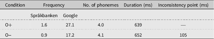
We assume that the frequency of a Swedish word is linked to the familiarity of a speaker of Danish with that particular word. Highly frequent words might therefore show smaller ERP components associated with the activation of orthography, which would distort the results if frequency structurally differed across conditions. Table 2 indicates mean frequency, number of phonemes, and duration across languages and conditions. As there are no up-to-date frequency lists for Swedish, frequency was assessed by averaging the number of hits in the Internet search engine Google and by averaging the number of hits in Korp (Borin, Forsberg & Roxendal Reference Borin, Forsberg and Roxendal2012). None of the features differed significantly across the two conditions. In total, the participants heard 56 O+ items, and 56 O– items. For each stimulus, the point of the inconsistency occurrence was determined. This was defined as the onset of the critical phonetic segment and was annotated in Praat (Boersma & Weenink Reference Boersma and David2008). For plosives, the onset was set between the silent interval and the noise burst.
Table 2. Mean values of stimulus features across conditions.
2.3 Procedure
The participants were seated in front of a computer screen. The words were presented auditorily in randomised order through loudspeakers placed in front of the participants. The participants were instructed to translate the word they heard into their native language and to type that translation on the keyboard, so that it appeared on the screen in front of them. In addition to the 112 experimental items, nine items were presented in a training block prior to the experiment. After this training block, participants were asked whether the task was clear and, if necessary, further instructions were given.
Every trial consisted of the following steps. A fixation cross was presented at the centre of the screen for 2000 ms to reduce the amount of head and conscious eye movements. The fixation cross remained on the screen during stimulus presentation and for 1500 ms after stimulus offset. After that, the fixation cross disappeared and a typing mask appeared in the centre of the screen. The time limit for typing in the translation was 10 seconds. The trial ended when the participants hit the enter key, or it ended automatically after this time limit. The participants were instructed to fixate the cross as long as it was presented, then to type in their translation.
2.4 EEG recordings
Continuous electroencephalogram (EEG) was recorded using Geodesic EEG Net Station software version 4.4.2 (EGI, Eugene, OR) with a 128-channel Geodesic Sensor Net (Tucker Reference Tucker1993). The impedance of all electrodes was kept below 50 kΩ prior to the recordings. All recordings were referenced to Cz online, then average-rereferenced off-line. Bioelectrical signals were amplified using a Net Amps 300 amplifier (EGI, Eugene, OR) and were continuously sampled (24-bit sampling) at a rate of 250 Hz throughout the experiment.
2.5 EEG data reduction and analyses
The electrode montage included four active midline sensors and four sensors over each hemisphere. In total, EEG responses to 112 stimuli were recorded from the 26 participants. From the resulting 2912 trials, those with incorrect translations were excluded from the analysis, as we intend to explore the processes underlying the (correct) identification of the stimulus. Including trials that resulted in wrong translations would therefore distort our data and potentially result in a type II error (the non-rejection of a false null hypothesis, also known as a ‘false negative’). In total, this resulted in the rejection of 43.5% of the trials for ERP analysis, leaving 1572 trials. From these remaining trials, those containing more than 10 bad channels or any ocular and muscular artefacts were further excluded (less than 3% of correct trials were excluded from the analyses). A semi-automated rejection algorithm was used for this purpose, together with a visual inspection procedure. EEG data were digitally filtered using a 0.3–30 Hz bandpass filter and averaged ERPs were formed off-line from correct trials free of ocular and muscular artefacts.
Continuous EEG data were divided off-line into epochs beginning 100 ms prior to target presentation and ending 1100 ms post-stimulus onset. Data were baseline corrected to a 100 ms pre-stimulus interval. ERPs were calculated by averaging the EEG time-locked to 100 ms before stimulus onset and lasting 2100 ms, i.e. from−100 ms to 2000 ms. The 100 ms pre-stimulus period was used as a baseline. Separate ERPs were formed for the two experimental conditions. Artefacts were screened using automatic detection methods (Net Station, Electrical Geodesics, Inc.). Segments containing eye blinks and movement artefacts were excluded from analyses. Bad channel data were replaced using spherical spline interpolation of neighbouring channel values (Perrin et al. Reference Perrin, Jacques, Bertrand and Jean1989). To select appropriate time windows for the ERP analyses, a preliminary stepwise analysis was performed comparing the mean amplitude obtained in the consistent condition with that of the inconsistent condition using pairwise t-tests. Mean amplitude was measured for 12 electrode sites (F3, Fz, F4, C3, Cz, C4, P3, Pz, P4, O1, Oz, O2; see Figure 1) in short and successive epochs, namely 12 epochs with a duration of 50 ms each, in the interval from 500 ms to 1100 ms after stimulus onset. This procedure allowed us to identify the precise moments at which the consistency effect appeared at different electrodes.

Figure 1. Schematic illustration of the topographic distribution of the twelve analysed sensors.
3. Results
3.1 Behavioural data
Mean correct reaction time and mean accuracy for both conditions are displayed in Table 3. Reaction times (RTs) were measured from stimulus onset to response offset, i.e. until the participants hit the enter key after having typed the translation. This resulted in relatively long RTs. RTs larger than three standard deviations (SDs) beyond the global mean of a participant were discarded (7.5% of the data), as were RTs to incorrect responses. While the accuracy scores were normally distributed (D(58) = 0.08, p = .2), the reaction times to correctly translated trials were not. Rather the latter were right-skewed (D(58) = 0.16, p = .001).
Table 3. Mean accuracy and median correct reaction time for both conditions.
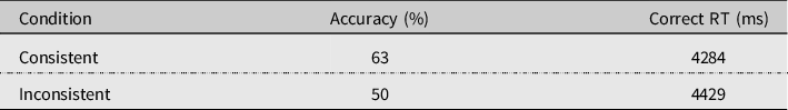
A pairwise t-test revealed that participants decoded items whose pronunciation was consistent to their cognates’ L1 orthography more accurately (65%) than inconsistent items (51%). This difference was highly significant (t(25) = 8.18, p < .001, r = 0.85).
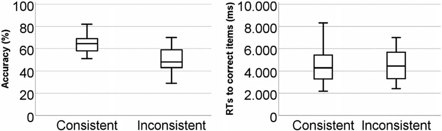
Figure 2. Boxplot of accuracy results (left) and correct reaction times (right) per condition.
Due to the non-normal distribution of the RT data, they were analysed using the non-parametrical Wilcoxon signed-rank test. Although the mean RTs to consistent items (Mdn = 4284 ms) were slightly shorter than those to inconsistent items (Mdn = 4429), this difference turned out not to be statistically significant (z = −1.41, p = .16, r = −0.20). Figure 2 illustrates the accuracy and the RT data.
3.2 EEG data
One of the first visible components was a central-posterior negativity (N1) peaking approximately 170 ms post-stimulus onset on Cz. The N1 was followed by a central-posterior positivity that peaked at about 300 ms (P2) at Cz. Following the P2, a negative-going wave was visible on centro-posterior electrode sites that peaked at about 520 ms.
Given previous research (e.g. Pattamadilok et al. Reference Pattamadilok, Perre, Dufau and Ziegler2008, Perre & Ziegler Reference Perre and Ziegler2008, Perre et al. Reference Perre, Pattamadilok, Montant and Ziegler2009), differences in mean amplitude across the two conditions could be expected in the time window 300–350 ms post-stimulus onset. However, as consistency effects in this time window are considered to reflect pre-lexical processing, we expect the effect to occur time-locked to the inconsistency. As the inconsistency in our material occurred somewhat earlier than in the cited studies, we analysed voltages recorded in a larger time window stretching from 200 ms to 350 ms. A repeated-measures ANOVA with the within-subject factors condition (two levels: O+, O−), laterality (three levels: left hemisphere, midline, right hemisphere) and anteriority (four levels: anterior, central, posterior, occipital) with Greenhouse-Geisser correction yielded no significant main effect for condition and no significant interaction effects of condition with laterality or anteriority, but an interaction effect of all three factors that approached significance (F(6,150) = 2.33, Greenhouse-Geisser p = .08). Inconsistency tended to elicit a negativity on right hemisphere electrodes (except for O2) and a positivity on occipital electrodes. Mean voltages per condition and electrode site are given in Table 4. These data are illustrated in Figure 3, which shows a scalp plot of difference waves (O− voltages minus O+ voltages) at 260 ms after stimulus onset.
Table 4. Mean voltages per condition and electrode site in the time window 200–350 ms post-stimulus onset.
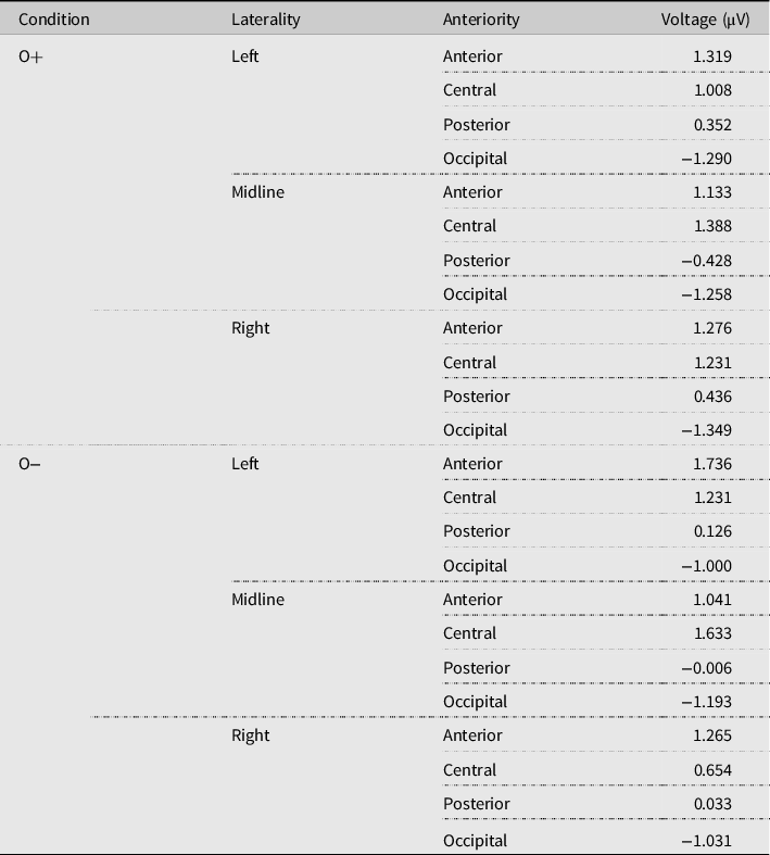

Figure 3. Voltage map based on difference waves (inconsistent minus consistent) at 260 ms post-stimulus onset.
A second time window in which main and interaction effects of condition have been reported (e.g. Pattamadilok et al. Reference Pattamadilok, Perre, Dufau and Ziegler2008, Perre & Ziegler Reference Perre and Ziegler2008, and Perre et al. Reference Perre, Pattamadilok, Montant and Ziegler2009) stretches from 500 ms to 750 ms post-stimulus onset. A repeated measures analysis of variance (ANOVA) yielded neither any significant main effect nor interactions in this time window. However, in the following time window from 750 ms to 900 ms post-stimulus onset, condition produced a significant main effect (F(1,25) = 15.47, p = .001) and a significant interaction with anteriority (F(3,75) = 3.64, p = .03). Mean voltages averaged across all electrode sites were 0.05 μV in the O+ condition and −0.62 μV in the O− condition, indicating a broadly distributed negativity for inconsistent items. Mean voltages per condition and per electrode site are displayed in Table 5, which shows that inconsistency elicited a positivity on anterior electrodes and a negativity on central, posterior, and occipital electrodes in this time window. This is further illustrated by a scalp plot in Figure 4.
Table 5. Mean voltages per condition and electrode site in the time window 750–900 ms post-stimulus onset.
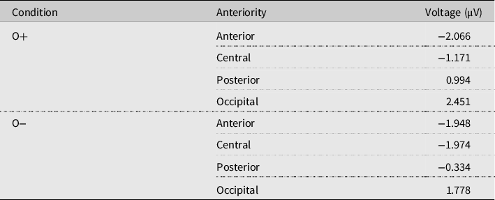

Figure 4. Voltage map based on difference waves (inconsistent minus consistent) at 820 ms post-stimulus onset.
Significance values for pairwise t-tests that were conducted for nine centro-posterior and occipital electrode sites in 16 subsequent time windows with durations of 50 ms each confirmed that a consistency effect was visible in two different time windows. A short positivity restricted to occipital electrodes occurred between 300 ms and 350 ms post-stimulus onset and a broadly distributed negativity on right and midline central and posterior electrodes was found between 750 ms and 1000 ms. These results are given in Table 6. Note that no post-hoc corrections of the alpha-level have been applied to this exploratory analysis. Grand average ERPs of the centro-posterior electrodes sites are presented in Figure 5. Figure 6 shows ERPs to inconsistent and consistent words at Cz and Figure 7 shows voltage maps based on difference waves (inconsistent minus consistent) at different times during word decoding.
Table 6. Time course of the consistency effect at 16 different electrode sites as confirmed by pairwise t-tests (*** p < .001, ** p < .01, * p < .05, - p > .05). Grey-shaded cells show significance values where inconsistency produced a negativity, black-shaded cells show significance values where inconsistency produced a positivity. No post-hoc corrections of the alpha-level have been applied.
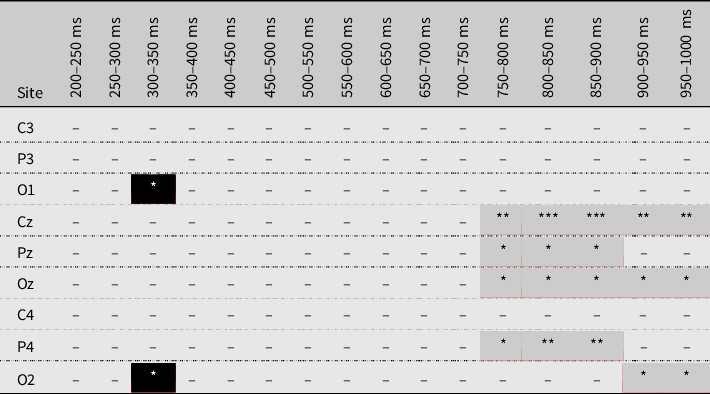

Figure 5. Grand-average ERPs (i.e. average voltage of all participants and all included trials) to inconsistent and consistent words at frontal (F3, Fz, F4), central (C3, Cz, C4), posterior (P3, Pz, P4) and occipital (O1, Oz, O2) electrode sites.

Figure 6. Grand-average ERPs to inconsistent and consistent words time-locked to word onset at Cz.

Figure 7. Voltage maps based on difference waves between inconsistent and consistent words.
4. Discussion
The earliest differences between inconsistent and consistent words in our data were found in the 200–350 ms time window. This finding is in line with Pattamadilok et al. (Reference Pattamadilok, Perre, Dufau and Ziegler2008), Perre & Ziegler (Reference Perre and Ziegler2008), and Perre et al. (Reference Perre, Pattamadilok, Montant and Ziegler2009), who typically reported an effect of orthographic inconsistency on centro-posterior and occipital electrodes in a 300–350 ms time window. In contrast to these studies, however, inconsistency did not elicit a negativity but a positivity. This effect only reached significance on two occipital electrodes in a pairwise t-test with condition as independent and voltage as dependent factor.
However, between 750 ms and 900 ms, the consistency effect reached significance across the whole time window, was broadly distributed topographically and highly significant, particularly in a smaller window stretching from 800 ms to 900 ms post-stimulus onset. Here, orthographically inconsistent items evoked significantly lower voltages, i.e. significantly more negative-going potentials on centro-posterior and occipital sites than consistent items did. The voltage differences across the two conditions were large enough as to also produce a significant main effect, i.e. if averaged across the scalp, voltages elicited by inconsistent items were more negative than for consistent items.
The fact that the second effect of consistency appeared about 300 ms later in our data than reported by Perre & Ziegler (Reference Perre and Ziegler2008) and Perre et al. (Reference Perre, Pattamadilok, Montant and Ziegler2009) could be because the task was more complex in our experiment. Both cited studies used a lexical decision task in which L1 French-speaking participants decided whether or not a word was a word in their native language, while participants in our experiment were confronted with a foreign language. Furthermore, a translation task can be assumed to require more resources and therefore cause longer latencies than decoding native language stimuli in a lexical decision task. This interpretation is supported by findings by Midgley et al. (Reference Midgley, Holcomb and Grainger2011), who report delayed lexical L2 access in a Go/No-go semantic categorisation task. The longer latency of the consistency effect compared to Perre & Ziegler (Reference Perre and Ziegler2008) could also indicate a late post-lexical or decisional locus of the orthography effect, which would be consistent with Pattamadilok, Perre & Ziegler’s (Reference Pattamadilok, Perre and Ziegler2011) interpretation of an orthographic effect in the time window 375–750 ms. The fact that inconsistent words produced a negativity that was maximal in 800–900 ms time window might be an indication that the inconsistency between L1 orthography and FL pronunciation is lexically resolved at this stage, or, rather, the consistency between L1 orthography and FL pronunciation is integrated into lexical retrieval.
Our data confirm that literacy, i.e. access to native orthography, changes the way the brain processes spoken words in a closely related language. Specifically, in the case of literate Danes confronted with spoken Swedish, this access enhances spoken word recognition of a closely related language. Our findings indicate that native orthography is not only involved in native-language spoken-word recognition, but also in non-native word recognition, if the two languages are closely related. Our findings thus expand findings by Pattamadilok et al. (Reference Pattamadilok, Perre, Dufau and Ziegler2008), Perre & Ziegler (Reference Perre and Ziegler2008), and Perre et al. (Reference Perre, Pattamadilok, Montant and Ziegler2009), who showed that L1 orthography is activated during L1 spoken word recognition, to the area of foreign language processing.
Recalling that Gooskens & Doetjes (Reference Gooskens and Gerard2009) reported that spoken Swedish is closer to written Danish than spoken Danish is to written Swedish, our results support the hypothesis that the asymmetry in mutual intelligibility between spoken Danish and Swedish, with Danes having fewer difficulties to decode spoken Swedish than vice versa (see Section 1) can at least partly be explained by differences in the depth of the speakers’ native orthographic systems. A more detailed account of the contribution of different phonemes and graphemes to the asymmetry is desired, but beyond the scope of this paper.
Danish has a more conservative orthography than Swedish, and, in recent centuries, spoken Danish has been developing further away from its East Nordic root than spoken Swedish (Elbro Reference Elbro, Malatesha Joshi and Aaron2006, Hjorth Reference Hjorth2018). Findings reported by Pharao (Reference Pharao2010) suggest that even today colloquial Danish is incorporating several reduction rules. The combination of these two factors (conservative orthography and ongoing syllable reduction during the last centuries until today) makes Danish orthography less transparent than Swedish orthography (Elbro Reference Elbro, Malatesha Joshi and Aaron2006). These differences may partly explain the finding reported by Elley (Reference Elley1992) and Seymour, Aro & Erskine (Reference Seymour, Mikko and Erskine2003), who showed that Danish children have more difficulties acquiring Danish orthography than their peers from other Nordic countries have. However, it seems that, once speakers of Danish finally have mastered the relatively non-transparent orthographic system of their native language, it serves as an additional cue for spoken language recognition in Swedish. Our findings confirm a strong link between literacy and spoken language processing not only for native but also for non-native target languages.
Acknowledgements
This work was supported by the Netherlands Organisation for Scientific Research (NWO 276-75-005), by the Institute of Language, Communication and the Brain (ANR-16-CONV-0002) and the Excellence Initiative of Aix-Marseille University (A*MIDEX). We are indebted to Kristina Borgström, who made sure the experiment as programmed abroad ran smoothly in the Humanities Lab. We also thank Jan Vanhove for help with the preparation of the material. Finally, we are grateful for extensive comments from three anonymous reveiwers on an earlier version of this manuscript, which helped to improve the quality of this report substantially.
APPENDIX
List of stimuli employed in the experiment


 Open access