


Introduction
The Groningen gas field production in the Dutch province of Groningen started in 1963. Since 1986, the region has experienced earthquakes with a maximum local magnitude (M L) of 3.6 (Huizinge event in 2012). During the Groningen earthquakes, energy is released at a depth of ~3 km (Buijze et al., Reference Buijze, van den Bogert, Wassing, Orlic and Veen2017; Van Elk et al., Reference van Elk, van Oeveren, Valvatne and Geurtsen2017; Visser and Solano Viota, Reference Visser and Solano Viota2017). Subsurface heterogeneities affect the radiation pattern by reflections and refractions. Additionally, the seismic energy is damped by spreading and friction, and possibly amplified at transitions to lower shear wave velocities (V S). The Groningen subsurface consists of up to an 800 m thick sequence of soft unconsolidated sediments that are mainly composed of sand and clay. Incorporating detailed schematisations of the geometry and characteristics of these layers are key factors in quantifying site response in the Ground Motion Models (GMM). Moreover, loosely packed sands at shallow depths (<20 m below the surface) can potentially liquefy upon earthquake shaking. Therefore, a detailed model of these sands is required to assess liquefaction potential. This paper describes two geological models: the ‘Geological model for Site response in Groningen’ (GSG model) and the ‘Geological model for Liquefaction sensitivity in Groningen’ (GLG model) respectively.
In the very first Ground Motion Model (GMM) constructed for Groningen after the 2012 Huizinge event (Bourne et al., Reference Bourne, Oates, Bommer, Dost, van Elk and Doornhof2015), the Groningen subsurface was characterised by a single value for shear wave velocity, averaged over the top 30 m (V S30), of 200 m s−1. This was justified by the necessity for a quick first assessment of the seismic hazard and risk in Groningen after the 2012 event. Since then, the GMM has become increasingly sophisticated (Bommer et al., Reference Bommer, Dost, Edwards, Stafford, van Elk, Doornhof and Ntinalexis2016). The aim of the GSG and GLG models was to provide geological information into the GMM and achieve a decrease in uncertainty in the seismic hazard and risk analysis related to the structure and composition of the subsurface.
General practice in site response analysis is to perform analyses for a relatively small area (e.g. a plant or a construction site) where the subsurface is characterised by a limited site characterisation study (e.g. Toro, Reference Toro1995; Rodriguez-Marek et al., Reference Rodriguez-Marek, Rathje, Bommer, Scherbaum and Stafford2014). The V S model usually extends to ~30 m depth. Uncertainty in the V S is accounted for by varying the V S models by 20–30% (e.g. Matasovic and Hashash, Reference Matasovic and Hashash2012; Griffiths et al., Reference Griffiths, Cox, Rathje and Teague2016). Three issues require a different approach for Groningen. The first is that the upper part of the subsurface of Groningen is very heterogeneous. Roughly speaking, the northern region contains up to 30 m of heterogeneous sediments (clay, sand and peat) of Holocene age while the southern region is dominated by sandy Pleistocene sediments. The architecture of the shallow subsurface is further complicated by local incising Holocene and Eemian tidal channels and small rivers draining the higher Pleistocene area. At depth, much wider and deeper subglacial valleys from the Saalian and Elsterian glaciations dominate local geological heterogeneity. Secondly, the amplification due to the soft soils is not limited to the top 30 m. Therefore, the reference bedrock horizon needs to be located much deeper. Thirdly, the region of interest is much larger than a single site, as the region spans over 1000 km2. The large amount of subsurface information available for this region allows for the construction of the GSG model, which includes a zonation model and parameterisations. The detailed 3D GeoTOP voxel model of TNO – Geological Survey of the Netherlands (Stafleu et al., Reference Stafleu, Maljers, Gunnink, Menkovic and Busschers2011, Reference Stafleu, Maljers, Busschers, Gunnink, Schokker, Dambrink, Hummelman and Schijf2012; Maljers et al., Reference Maljers, Stafleu, Van der Meulen and Dambrink2015; Stafleu & Dubelaar, Reference Stafleu and Dubelaar2016) forms the basis of the GSG model. Properties such as V S, overconsolidation ratio (OCR) and plasticity index (I p) are assigned to the voxels. The GSG model feeds into site response calculations (Rodriguez-Marek et al., Reference Rodriguez-Marek, Kruiver, Meijers, Bommer, Dost, van Elk and Doornhof2017) that are part of GMM (Bommer et al., Reference Bommer, Dost, Edwards, Stafford, van Elk, Doornhof and Ntinalexis2016, Reference Bommer, Dost, Edwards, Kruiver, Ntinalexis, Rodriguez-Marek, Stafford and van Elk2017, in press). The incorporation of geology into the Groningen GMM via the GSG model resulted in a major improvement (Bommer et al., Reference Bommer, Dost, Edwards, Stafford, van Elk, Doornhof and Ntinalexis2016, Reference Bommer, Dost, Edwards, Kruiver, Ntinalexis, Rodriguez-Marek, Stafford and van Elk2017, in press).
So far, liquefaction has not been incorporated into the seismic hazard and risk analysis for Groningen. In order to assess the need to incorporate liquefaction, the potential sensitivity of Groningen soil to liquefaction upon shaking at the levels of possible future earthquakes needs to be established. Liquefaction severity is generally assessed using damage index frameworks, such as Liquefaction Potential Index (LPI). LPI is based on liquefaction evaluations performed using the simplified procedure (e.g. Idriss & Boulanger, Reference Idriss and Boulanger2008) on relatively small datasets of cone penetration tests (CPT). In the Groningen case, there is a large dataset of ~5,700 CPT soundings available extending down to an average depth of ~20 m. These were interpreted in terms of GeoTOP model units and relative densities which serve as proxies for the packing of the sand per model unit. The results were used to determine the cumulative thickness of loosely packed sand and its lateral extent and variation.
In the following two sections, the geological setting of the Groningen gas field region is described, followed by a description of the high-resolution GeoTOP model. The next section illustrates the use of the GeoTOP and deeper geological models in the GSG model and the use of GeoTOP in the GLG model. The same section includes the parameterisation of both models. In the final section, we discuss potential improvements in the input data, the geological modelling and model parameterisation steps.
Geological setting of the Groningen gas field area
The geology of the Groningen gas field area is illustrated using a representative transect from Oosterwolde in the southwest, to Delfzijl and part of the Wadden Sea in the northeast. The transect depicts data from the GeoTOP model (Fig. 1A), the Digital Geological Model (DGM; Gunnink et al., Reference Gunnink, Maljers, Van Gessel, Menkovic and Hummelman2013; Fig. 1B) and the Digital Geological Model Deep (TNO, 2016; Fig. 1C). A 3D overview of the shallow geology is shown as a series of GeoTOP maps (Figs 2, 3). The location of the transect is shown in Figure 3. All geological models are constructed and maintained by TNO – Geological Survey of the Netherlands.

Fig. 1. Transect through the geological models, from Oosterwolde to Delfzijl extending into the Wadden Sea: (A) GeoTOP model (version 1.3); (B) Digital Geological Model (version 2.2; Gunnink et al. Reference Gunnink, Maljers, Van Gessel, Menkovic and Hummelman2013); (C) Digital Geological Model Deep (version 4.0; TNO, 2016). The abbreviations for Groups, Formations and Members are included in Table 1. The position of the transect is indicated in Figure 3. All models can be accessed on www.dinoloket.nl.

Fig. 2. GeoTOP lithostratigraphical units: (A) Peelo Formation; (B) Drente Formation; (C) Eem Formation; (D) Boxtel Formation; (E) Nieuwkoop Formation, Basal Peat Bed; (F) Naaldwijk Formation, Wormer Member and Nieuwkoop Formation, Hollandveen Member; (G) Naaldwijk Formation, other Members; (H) Man-made ground and Nieuwkoop Formation, Griendtsveen Member. Each panel is included in the electronic supplement (https://doi.org/10.1017/njg.2017.11).
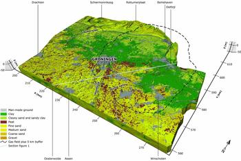
Fig. 3. GeoTOP lithological class. The location of the transect of Figure 1 is indicated by the blue line between Oosterwolde and Delfzijl. A figure including both lithological class and lithostratigraphical units is included in the electronic supplement (https://doi.org/10.1017/njg.2017.11).
Pre-Quaternary
Sediments of the Upper-Rotliegend Group represent the main reservoir of the Groningen gas field. This unit is overlain by ~2200 m of the Zechstein, Lower- and Upper Germanic Trias, Rijnland and Chalk Groups (Fig. 1C). Shallow marine glauconitic sediments of the Middle and Lower North Sea Group occur on top of the late Palaeozoic and Mesozoic sequence. The base of the Lower North Sea Group, defining the lower boundary of site response in the Groningen area, is, on average, positioned around 800 m below the Dutch datum NAP (Fig. 1C), although much shallower depths occur at locations of salt diapiric structures. The lower part of the overlying Upper North Sea Group sediments consists of ~150 m of marine, clayey glauconitic sediments of the Miocene age Breda Formation (Fig. 1B). In the Late Miocene, the Netherlands was situated at the southern rim of the Eridanos Delta (Zagwijn, Reference Zagwijn1989; Overeem et al., Reference Overeem, Weltje, Bishop-Kay and Kroonenberg2001). This delta was the terminal zone of a river system draining large parts of the Baltic area. The major part of the Eridanos fluvio-deltaic wedge consists of marine shelf deposits, in the Groningen gas field region reflected by ~100 m of sediments of the Pliocene age Oosterhout Formation (Fig. 1B).
Quaternary
Activity of the Eridanos River system continued into the Quaternary, resulting in deposition of up to ~50 m of marine shelf sediments (Maassluis Formation; Fig. 1B) and ~100 m of coarse-grained fluvial sands with limited occurrence of fine-grained intercalations (combined Peize–Waalre Formations; Fig. 1B). Activity of this river system terminated at the end of the Early Pleistocene as a result of glaciation in its catchment area (Bijlsma, Reference Bijlsma and van Loon1981). Following termination of the Eridanos, deposition of sediment from northern Germany and Poland (Appelscha Formation; Fig. 1A, B) continued until well into the Middle Pleistocene. Sedimentary information from quarries as well as the presence of Fennoscandian erratics, shows that the upper part of this formation, occurring at 40–50 m depth in the Groningen region, was deposited in close proximity to an ice sheet (Ruegg & Zandstra, Reference Ruegg and Zandstra1977; Lee et al., Reference Lee, Busschers and Sejrup2012). Following an interglacial period marked by the deposition of fine-grained, near-coastal sediments and deposition of Rhine sediments in the west of the area (Urk Formation, Veenhuizen Member; Fig. 1A), the northern Netherlands were glaciated during the Elsterian glaciation (~450,000 or ~350,000 years ago; Lee et al., Reference Lee, Busschers and Sejrup2012). The Elsterian glaciation left a major imprint on the shallow geology in the Groningen region by the formation of up to ~375 m deep subglacial valleys and deposition of subglacial, fluvio-glacial and glacio-lacustrine sediments (Bosch, Reference Bosch1990; Kluiving et al., Reference Kluiving, Bosch, Ebbing, Mesdag and Westerhoff2003). The valley infill consists of a coarse-grained deeper part that fines upward to fine-grained sands and two or three levels of characteristic stiff, black to brown clays (‘potklei’ in Dutch). Outside the tunnel valleys, the Peelo Formation is mainly composed of fine-grained sand as well as the upper potklei level (Peelo Formation; Figs 1 A, B, 2A). Locally, coarse-grained sediments occur in the upper part of the Peelo Formation as well, although further study is needed to determine their exact stratigraphic position. In the Groningen gas field region, the sediments of the Peelo Formation make up about 60% of all sediments present between the surface and 50 m depth.
After the Elsterian, some of the deep valleys were further infilled with fine-grained estuarine sediments and locally peat (Urk Formation, Tynje Member) while in higher areas erosion prevailed. Significant deposition occurred again only at the onset of the Late Saalian period between 190,000 and 170,000 years ago (Kars et al., Reference Kars, Busschers and Wallinga2012) with the deposition of local river and aeolian sediments in the western part of the region (Drachten Formation, Fig. 1A, B). The region was glaciated again about 170,000 years ago (Drente substage glaciation; Van den Berg & Beets, Reference van den Berg and Beets1987; Busschers et al., Reference Busschers, Van Balen, Cohen, Kasse, Weerts, Wallinga and Bunnik2008). Initially, ice-sheet progradation occurred in a NE–SW direction, but in a later phase this changed towards a NW–SE direction. This created a series of NW–SE-oriented elongated hills (‘megaflutes’) of which the Hondsrug is the largest (Van den Berg & Beets, Reference van den Berg and Beets1987). The location of the Hondsrug is indicated in Figure 3. In contrast to the Elsterian, the Drente substage glaciation was characterised by deposition of a glacial till, which is especially well preserved in the western part of the region (Drente Formation, Gieten Member; Figs 1A, B, 2B).
A vast incised valley system was carved east of the Hondsrug during deglaciation. Incision of this Hunze valley system occurred up to 60 m depth and was followed by the infill with coarse-grained and gravelly sediments (Drente Formation, Schaarsbergen Member; Figs 1A, B, 2B). The top of this unit gradually changes to medium- and fine-grained sands. During the Eemian interglacial, between 122,000 and 115,000 years ago (Sier et al., Reference Sier, Peeters, Dekkers, Parés, Chang, Busschers, Wallinga, Cohen, Bunnik and Roebroeks2015), an estuary developed within the former valley system (Figs 1A, 2C). The Eem Formation contains both clay and peat layers. Locally, this unit is composed of coarse sand due to erosion of older sediment. During the Weichselian period, in particular during the period 60,000–15,000 years ago, the Hunze valley system was largely infilled with local river sediments consisting of medium- and fine-grained sands and intercalated loam and peat layers (Boxtel Formation; Figs 1A, 2D). In the higher areas east and west of the Hunze valley, small river valleys dissected the former glacial landscape (Boxtel Formation, Singraven Member 2, Figs 1A, 2D). At the end of the Weichselian, the entire region was covered by an up to 3 m thick veneer of aeolian sediments (Fig. 1A). In higher areas like the Hondsrug, the aeolian sediments were removed by erosion afterwards, resulting in local exposure of older Middle Pleistocene sediments.
Holocene
In the early Holocene, large-scale peat formation occurred on top of the gently sloping Pleistocene surface (Nieuwkoop Formation, Basal Peat Bed; Figs 1A, 2E). This peat bed has a maximum thickness of 2 m and is a key stratigraphic marker at the base of the Holocene sequence where no younger channel erosion occurred. Peat formation was driven by sea-level rise and related rise in groundwater level following melting of the Weichselian ice sheets. In the lower parts of the landscape, peat formation was gradually replaced by sedimentation of humic clays that deposited under brackish conditions (Naaldwijk Formation, Wormer Member; Figs 1A, 2F). Ongoing sea-level rise led to continuing onlap of the former Pleistocene landscape and development of a large tidal basin (Naaldwijk Formation, Wormer Member; Figs 1A, 2F) with coastal barriers and tidal inlets in the north and tidal lagoons along the most landward part of the tidal area. Along the fringes of the tidal basin, sediments of the Wormer Member were gradually covered with peat (Nieuwkoop Formation, Hollandveen Member; Fig. 2F), while further north the tidal inlets remained an open and active system (Fig. 1A). The latter is a key difference between tidal basins in the western part of the Netherlands which became almost entirely covered with peat during this phase (Beets & Van der Spek, Reference Beets and van der Spek2000; Vos, Reference Vos2015). The Hunze valley, small river valleys and surrounding Pleistocene areas were gradually covered by an up to several metres thick peat layer (Nieuwkoop Formation, Griendtsveen Member (Fig. 2H) and Boxtel Formation, Singraven Member 1).
Following a period of ongoing peat formation, Late Iron Age and Roman reclamation activities and peat mining initiated peat-surface lowering (Vos, Reference Vos2015; Pierik et al., Reference Pierik, Cohen, Vos, van der Spek and Stouthamer2017). As a result, renewed ingressions of the North Sea occurred, leading to inland deposition of clayey tidal sediments (Naaldwijk Formation, Walcheren Member; Figs 1A, 2G) on top of the peats (Roeleveld, Reference Roeleveld1974; Vos & Knol, Reference Vos and Knol2015; Pierik et al., Reference Pierik, Cohen, Vos, van der Spek and Stouthamer2017). Increase in back barrier tidal volumes led to formation and gradual enlargement of tidal inlets like the Lauwerszee, while, along the tidal basin fringes, subtidal and supratidal (marsh) environments existed (Vos, Reference Vos2015). After ~AD 1000, embankment of the then silted-up tidal areas resulted in the sand-dominated Wadden Sea as the only active tidal area.
GeoTOP
TNO – Geological Survey of the Netherlands (TNO-GSN) systematically produces 3D geological models of the Dutch subsurface (Van der Meulen et al., Reference van der Meulen, Doornenbal, Gunnink, Stafleu, Schokker, Vernes, Van Geer, Van Gessel, Van Heteren, Van Leeuwen, Bakker, Bogaard, Busschers, Griffioen, Gruijters, Kiden, Schroot, Simmelink, Van Berkel, Van der Krogt, Westerhoff and Van Daalen2013). One of these models is the voxel model GeoTOP, which describes the geometry and properties of the shallow subsurface to a maximum depth of NAP −50 m (Stafleu et al., Reference Stafleu, Maljers, Gunnink, Menkovic and Busschers2011, Reference Stafleu, Maljers, Busschers, Gunnink, Schokker, Dambrink, Hummelman and Schijf2012; Maljers et al., Reference Maljers, Stafleu, Van der Meulen and Dambrink2015; Stafleu & Dubelaar, Reference Stafleu and Dubelaar2016). GeoTOP schematises the subsurface in a regular grid of rectangular blocks (‘voxels’, ‘tiles’ or ‘3D grid cells’) each measuring 100 m × 100 m × 0.5 m (x, y, z). Each voxel in the model contains estimates of the lithostratigraphical unit and the representative lithological class (including a grain-size class for sand) (see Table 1). The estimates are calculated using stochastic techniques that allow the construction of multiple, equally probable 3D realisations of the model as well as an evaluation of model uncertainty (Stafleu et al., Reference Stafleu, Maljers, Gunnink, Menkovic and Busschers2011). A ‘most likely’ subsurface model was determined from the multiple subsurface models and subsequently used in the GSG model. The GeoTOP model (version 1.3) is publicly available at www.dinoloket.nl/en/subsurface-models (Stafleu & Dubelaar, Reference Stafleu and Dubelaar2016).
Table 1. Lithostratigraphical units from the GeoTOP model, Digital Geological Model and Digital Geological Model Deep.
a Units not formally defined in the lithostratigraphical nomenclature of the shallow subsurface.
b In this region this unit corresponds to the Schaarsbergen Member. The depositional domain and main composition of each unit is included in the electronic supplement (https://doi.org/10.1017/njg.2017.11).
The GeoTOP model of the northeastern part of the Netherlands (‘Oostelijke Wadden’), including the Groningen region, is shown in Figures 2 and 3. Figure 2 shows the succession of units, and Figure 3 shows the lithoclass model.
Data
The GeoTOP model in the Groningen region was constructed using ~42,300 digital borehole descriptions from DINO, the national Dutch subsurface database operated by the Geological Survey. The largest part of these boreholes consists of manually drilled auger holes. As a result, borehole density decreases rapidly with depth. This implies that, in general, model uncertainty also increases with depth.
The upper boundary of the model is derived from the 5 m × 5 m cell-size national airborne laser altimetry survey dataset (AHN2 – Actueel Hoogtebestand Nederland; www.ahn.nl). Information on water depths of rivers, canals, Eemshaven and the Wadden Sea was obtained from bathymetric survey data. Other information at or close to the land surface comes from the soil map 1:50,000 (Steur & Heijink, Reference Steur and Heijink1991; de Vries et al., Reference de Vries, de Groot, Hoogland and Denneboom2003), the geomorphological map 1:50,000 (Koomen & Maas, Reference Koomen and Maas2004) and the national land use map (LGN5 – Landelijk Grondgebruik Nederland, developed and maintained by Alterra). The Digital Geological Model (version 2.2; Gunnink et al., Reference Gunnink, Maljers, Van Gessel, Menkovic and Hummelman2013) was used to define the maximum lateral extent of selected lithostratigraphical units. The maximum lateral extent of the Drente Formation, Gieten Member (glacial till) unit and the procedure to identify the unit in the borehole descriptions were largely based on the large-scale and detailed till model for the north of the Netherlands (Vernes et al., Reference Vernes, Bosch, Harting, Maljers and Schokker2013).
Modelling procedure
The first step in the modelling procedure is a geological schematisation of the borehole descriptions into units that have uniform sediment characteristics, using lithostratigraphical and lithological criteria. In the second modelling step, the lithostratigraphical interpretation of the borehole descriptions is used to construct 2D surfaces representing the top and base of the lithostratigraphical units. These are used to assign the most likely lithostratigraphical unit to each voxel in the model (Fig. 2). Finally, the lithological classes in the borehole descriptions are used to perform a 3D stochastic interpolation of lithological class (clay, sand, peat) and, if applicable, sand grain-size class within each lithostratigraphical unit. After this step, a 3D geological model is obtained (Fig. 3). Details of the modelling procedure are described in the following subsections.
Lithostratigraphical and lithological interpretation of borehole descriptions
The first step in the lithostratigraphical interpretation of borehole descriptions is the identification of the units present in the model area. This identification is based on geological knowledge of the area combined with data from boreholes and expert judgement. The second step is to assign a lithostratigraphical interpretation to the borehole descriptions. To do so, two automated procedures were developed. The first is a simple intersection of the boreholes with the top and the basal raster layers of the DGM model units and assignment of the borehole intervals with the corresponding DGM lithostratigraphy. The second procedure is more sophisticated and is based on borehole descriptions. It consists of the iterative improvement of maps showing the maximum lateral extent of model units and criteria for the translation of borehole descriptions to lithostratigraphical units. This more sophisticated procedure was applied to all Holocene units (i.e. anthropogenic deposits through Nieuwkoop Formation, Basal Peat Bed) and three of the Pleistocene units: Boxtel Formation, Wierden and Singraven Members, and Drente Formation, Gieten Member. These units were successfully interpreted using automated procedures, because their lithological composition contrasts strongly with overlying and underlying units. For instance, the peat of the Holland Peat Member is easily recognised, because it is embedded in the fine sands and clays of the tidal deposits of the Walcheren and Wormer Members. In the resulting lithostratigraphical interpretation, the more sophisticated result based on borehole descriptions overruled the result derived from the DGM model.
Additionally, lithological information for each borehole interval was obtained from the borehole descriptions, including main lithology, admixtures of sand, silt and clay, sand median and shell content. Based on these attributes, each borehole interval was assigned a lithological class following the lithological classification scheme used in the hydrogeological subsurface model REGIS II (version 2.1, Vernes & Van Doorn, Reference Vernes and Van Doorn2005). The lithological classes are anthropogenic deposits, organic deposits (peat), clay, clayey sand and sandy clay, fine sand (median grain size 63–150 μm), medium sand (median grain size 150–300 μm) and coarse sand, gravel and shells (median grain size >300 μm).
2D interpolation of lithostratigraphical surfaces
The base levels of the lithostratigraphical units found in the boreholes were interpolated to regular grids with a cell size of 100 m × 100 m using Sequential Gaussian Simulation (Goovaerts, Reference Goovaerts1997; Chilès & Delfiner, Reference Chilès and Delfiner2012). The simulations were carried out using the Isatis® modelling software package of Geovariances and resulted in 100 different realisations of statistically equally probable surfaces of the base of the lithostratigraphical units. From these realisations, mean base surfaces were calculated and subsequently used to construct a single, integrated layer model that takes into account the stratigraphical order of the units as well as their cross-cutting relationships. In order to prevent removal of thin key model units, a minimum thickness of just over half a voxel thickness (0.3 m) was specified for these units. The final 2D layer model of basal and top surfaces was used to assign the corresponding lithostratigraphical unit to each voxel within the 3D model space (Fig. 2).
3D interpolation of lithological class
The lithological classes in the boreholes were used as input for a 3D stochastic simulation procedure within each lithostratigraphical unit. The Sequential Indicator Simulation technique (SIS; Goovaerts, Reference Goovaerts1997; Chilès & Delfiner, Reference Chilès and Delfiner2012) was applied using the Isatis® modelling software package of Geovariances. SIS estimates lithological classes for each voxel within a particular lithostratigraphical unit based on the lithological class of the surrounding borehole intervals of the same lithostratigraphical unit. The simulation was repeated 100 times, resulting in 100 statistically equally probable realisations of 3D lithological class distribution. From these realisations a ‘most likely lithological class’ was derived using the averaging method for indicator datasets (Soares, Reference Soares1992; Fig. 3).
For specific heterogenetic units, a Vertical Proportion Curve was applied describing the expected proportion of sand and clay as a function of depth. Additionally, the impermeable clay layers within the Peelo Formation were modelled using raster layers from the hydrogeological model REGIS II (version 2.1, Vernes & Van Doorn, Reference Vernes and Van Doorn2005). Voxels within these layers were assigned a high expected proportion of clay.
Applications of GeoTOP and deeper models
Geological model for site response
Amplification of earthquake motions is to be expected in the presence of shallow soft sediments. The vertical succession of unconsolidated sediments in Groningen amounts to several tens to hundreds of metres. The distribution of sediment types and associated properties, however, is not uniform. Accordingly, geographically varying site response is to be expected due to the geological heterogeneity. Although it is not possible to predict the succession at each individual location, we were able to define zones of similar geological successions based on their presence in GeoTOP. Geological features that are smaller than the GeoTOP voxel sizes, such as creeks with a width of less than 10 m, are included in an indirect way. These small-scale features are encountered in boreholes, and therefore statistically present in GeoTOP voxels.
The zonation is based on typical successions of geological units in the top tens of metres of the GeoTOP model (Stafleu et al., Reference Stafleu, Maljers, Gunnink, Menkovic and Busschers2011, Reference Stafleu, Maljers, Busschers, Gunnink, Schokker, Dambrink, Hummelman and Schijf2012; Maljers et al., Reference Maljers, Stafleu, Van der Meulen and Dambrink2015; Stafleu & Dubelaar, Reference Stafleu and Dubelaar2016), because the site response is expected to be dominated by the composition of the shallow sediments. A first draft of a geological zonation map was created by overlying the lateral extents of the geological units. This resulted in a patchwork map of large and small polygons. Next, the boundaries of these polygons were adjusted based on additional data from the 19,082 borehole descriptions from the DINO database (www.dinoloket.nl), 5,674 CPT soundings, DGM (Gunnink et al., Reference Gunnink, Maljers, Van Gessel, Menkovic and Hummelman2013), REGIS II (version 2.1, Vernes & van Doorn, Reference Vernes and Van Doorn2005), the digital terrain model AHN (open data, www.ahn.nl), and palaeogeographic maps (Vos et al., Reference Vos, Bazelmans, Weerts and Van der Meulen2011; Vos & Knol, Reference Vos and Knol2015). Small polygons were combined to obtain a minimum of 50 grid cells per zone. Large polygons were split if properties, such as the thickness of a peat layer, varied too much within one polygon. In this case, a polygon was split into two or more zones. Some zones consist of multipart polygons, meaning that the different parts of the zone are not adjoined, but cut by other zones. The resulting geological zonation map is shown in Figure 4 (Kruiver et al., Reference Kruiver, van Dedem, Romijn, de Lange, Korff, Stafleu, Rodriguez-Marek, van Elk and Doornhof2017). The colours indicate the typical succession of geological units. For example, blue indicates the classical Holocene succession of the Walcheren Member (Naaldwijk Formation), Holland peat Member (Nieuwkoop Formation), Wormer Member (Naaldwijk Formation) and Basal peat bed (Nieuwkoop Formation). The different shades of blue indicate the presence or absence of Eem Formation or the Gieten Member (Drente Formation).

Fig. 4. Geological zonation (thin grey lines) of the Groningen field (bold grey line) with a 5 km buffer around it (bold blue line). Similar colours indicate similar typical successions of geological units (Kruiver et al., Reference Kruiver, van Dedem, Romijn, de Lange, Korff, Stafleu, Rodriguez-Marek, van Elk and Doornhof2017).
Site response calculations are required to start at a reference baserock horizon. Below that level, the earth is considered to be a uniform elastic half-space. In the latest GMM (Bommer et al., Reference Bommer, Dost, Edwards, Stafford, van Elk, Doornhof and Ntinalexis2016, Reference Bommer, Dost, Edwards, Kruiver, Ntinalexis, Rodriguez-Marek, Stafford and van Elk2017), the reference baserock horizon is positioned at the base of the North Sea Supergroup at ~800 m depth. Therefore, the geological model is extended from the GeoTOP range at NAP–50 m down to the base of the North Sea Group. The amount of information about the composition quickly decreases with increasing depth. It is therefore not possible to make a detailed geological model of the deeper layers. Some lithostratigraphical units, e.g. the valleys of the Peelo Formation, are expected to have a profound effect on the site response based on their geomechanical properties. It is, however, rarely known exactly where they are located, due to the limited data density in relation to their strong lateral variation. Nevertheless, it is possible to determine the probability of encountering a Peelo channel or other stratigraphic successions in a certain area. A scenario-based approach was chosen to cope with this uncertainty (Hijma et al., Reference Hijma, van der Meij, Lam, Schweckendiek, Van Tol, Pereboom, Staveren and Cools2015, Reference Hijma, Lam and van der Hammen2016). A zonation map and corresponding scenarios were defined for the geology below NAP-50 m based on geological architecture and lithological variation. The ‘deep’ zonation map differs from the zonation in Figure 4, because the geology below NAP-50 m is different from the shallow geology.
The layer profiles of the full depth range from surface to the base of the North Sea Supergroup are a combination of the GeoTOP voxel stacks and the deeper scenarios. Each GeoTOP voxel stack is extended using one randomly selected scenario from the deep zone at that location, while satisfying the probabilities of the different scenarios within that deep zone. If, for example, two scenarios are defined within a specific zone with probabilities of 60% and 40% respectively, then 60% of the voxel stacks are combined with the first scenario and 40% of the voxel stacks are combined with the second scenario. The coordinates of the voxel stacks within that zone that receive either the first or the second scenario are randomly chosen. The combination of the GeoTOP voxel stacks and the scenarios results in one stratigraphy–lithology column for each coordinate in the field on a 100 m × 100 m grid. In total, ~140,000 voxel stacks are defined in the Groningen field using this approach. Uncertainty in soil profiles was accounted for by assuming that all possibilities within a zone are represented by the voxel stacks within that zone. A minimum of 50 voxel stacks in a geological zone ensures adequate sampling of soil profiles. The median size of the geological zones is 537 voxel stacks.
The amount of information available at depth and the effect on the site response is visualised in Figure 5. The amount of information decreases with depth, as does the influence of subsurface variations on site response. The GSG model uses a probabilistic approach for the top of the model, where the influence on the site response is largest. Not only the layering model is input to site response analyses, but also the parameters attributed to these layers. One of the inputs for site response calculations is a depth profile of V S. The other input consists of geomechanical properties of the layers that define the nonlinear soil behaviour in the form of modulus reduction and damping curves. Similar to the layering information, the amount of available information for relevant parameters decreases with depth. When data allowed, we adopted a stochastic approach, for example for the top 50 m of the V S profile. For other parameters, the uncertainty was accounted for in the sigma model of the GMM (Bommer et al., Reference Bommer, Dost, Edwards, Stafford, van Elk, Doornhof and Ntinalexis2016, Reference Bommer, Dost, Edwards, Kruiver, Ntinalexis, Rodriguez-Marek, Stafford and van Elk2017, in press) and deterministic values were used.

Fig. 5. Visualisation of the coupling of depth ranges in the geological model and the relation between the level of information, the influence of the depth range on site response and the adopted probabilistic or deterministic approach. NU_B is the base of the Upper North Sea Group; NS_B is the base of the North Sea Supergroup.
For the Groningen field, a V S model was constructed partially based on the GSG model. The V S model is a combination of the splicing of three models over three depth ranges (Kruiver et al., Reference Kruiver, van Dedem, Romijn, de Lange, Korff, Stafleu, Rodriguez-Marek, van Elk and Doornhof2017). The V S model between the surface and NAP-50 m is based on the GeoTOP model. The V S model in the depth range between NAP-50 m and max NAP-120 m is based on the inversion of surface waves from the seismic reflection survey that was conducted in the 1980s to image the reservoir. The V S model between ~NAP-70 m and the base of the North Sea Supergroup is formed by the conversion from small-strain primary wave velocities (V P) to V S of the PreStack Depth Migration Model from the seismic reflection survey. The reader is referred to Kruiver et al. (Reference Kruiver, van Dedem, Romijn, de Lange, Korff, Stafleu, Rodriguez-Marek, van Elk and Doornhof2017) for additional information about the deeper models. The shallow V S model of Kruiver et al. (Reference Kruiver, van Dedem, Romijn, de Lange, Korff, Stafleu, Rodriguez-Marek, van Elk and Doornhof2017) is explained here, because it is an illustration of the application of the GeoTOP model.
In general, the value of V S varies with lithostratigraphy, lithology and depth. For example, Holocene tidal deposits have different properties than deposits which have experienced loading by ice sheets. Additionally, sand has generally higher V S than clay. A set of 88 SCPT soundings is available for Groningen. Part of these SCPT soundings was acquired during a fieldwork campaign aimed at characterising the KNMI accelerograph stations in Groningen (de Kleine et al., Reference de Kleine, Noorlandt, de Lange, Karaoulis and Kruiver2016). Active Multichannel Analysis of Surface Waves (MASW), SCPT and, in some cases, down-hole and cross-hole V S measurements were performed at 18 KNMI accelerograph station sites. All SCPT data were classified in terms of stratigraphy and lithology. The V S values for each combination of stratigraphy and lithology (‘unit’ for short) were assembled. For each unit, the statistics of the V S distribution were determined. This was either in the form of V S dependence on mean effective confining stress or a constant V S. In both cases, an uncertainty band was defined. For units not represented in the SCPT dataset, characteristics of a similar unit or literature values (Wassing et al., Reference Wassing, Maljers, Westerhoff, Bosch and Weerts2003) were assigned to the unit.
In order to create the V S profiles as input for the site response calculations, the V S distributions were combined with the GeoTOP model. The resulting 3D image of the mean V S model is shown in Figure 6. It shows the clear distinction between high velocities in the south and low velocities in the north near land surface (Fig. 6b). When all deposits younger than the Peelo Formation are removed from the model (Fig. 6a), the heterogeneity of the Peelo, Urk and Appelscha Formations with high and low V S is clear. The site response calculations are based on randomised V S profiles in order to account for uncertainty in V S (Rodriguez-Marek et al., Reference Bommer, Dost, Edwards, Kruiver, Ntinalexis, Rodriguez-Marek, Stafford and van Elk2017). Randomised V S profiles were created by sampling from the distributions with full correlation within one unit in a voxel stack and partial correlation (coefficient of 0.5) between different units in one voxel stack (Kruiver et al., Reference Kruiver, van Dedem, Romijn, de Lange, Korff, Stafleu, Rodriguez-Marek, van Elk and Doornhof2017). This means that the V S values of all, say, Naaldwijk clay layers within one voxel stack are fully correlated. When a different unit in the same voxel stack is encountered (e.g. a Basal Peat layer below a Naaldwijk clay layer), a new sample of V S is taken for the new unit which is linked to the former by a correlation coefficient 0.5.

Fig. 6. 3D view of GeoTOP attributed with VS: (A) the model where all strata younger than the Peelo Formation are removed; (B) the full model from NAP −50 m up to land surface.
Although V S is an important parameter in the site response calculations, the dynamic soil behaviour is described by modulus reduction and damping curves which are defined by geomechanical parameters. For clay, these parameters are OCR, I p, undrained shear strength (Su), and total unit weight for clay (Darendeli, Reference Darendeli2001). For sand, these parameters are median grain size (D 50), coefficient of uniformity (C u) and total unit weight (Menq, Reference Menq2003). To determine the values for various geomechanical parameters, SCPT and CPT data were classified in terms of lithostratigraphical unit using GeoTOP and lithoclass using a Groningen-specific classification chart based on the cone resistance vs friction ratio following Douglas & Olsen (Reference Douglas and Olsen1981). OCR, S u and total unit weight were estimated for stratigraphic units and lithoclasses using literature relations between cone resistance and these parameters (Kulhawy & Mayne, Reference Kulhawy and Mayne1990; Robertson, Reference Robertson1990; Lunne et al., Reference Lunne, Robertson and Powell1997). Additionally, I p was estimated from CPT data using Skempton & Henkel (Reference Skempton and Henkel1953), from scarce site investigation data from Rijkers et al. (Reference Rijkers, Huisman, De Lange, Weijers and Witmans-Parker1998) and Sorensen & Okkels (Reference Sorensen and Okkels2013), and from expert judgement. Information on D 50 and C u for sand was provided by the inventory performed by TNO-GSN (Bosch et al., Reference Bosch, Harting and Gunnink2014), which contains a large number of grain-size analyses for almost all units. An example of the derivation of Groningen-specific parameters is given in Figure 7. The tip resistance q c was transformed to S u and plotted vs vertical effective stress for clay of the Peelo Formation. The regression line defines the S u for Peelo clay in the soil profiles. In general, characteristics of similar units were assumed for units not represented by the CPT data or literature.

Fig. 7. Example of derivation of Groningen specific soil parameters from CPT soundings: Su for clay of the Peelo Formation. The grey line indicates the linear regression line based on 52,337 data points and R2 = 0.57.
Geological model for liquefaction susceptibility
Until now, the liquefaction sensitivity of the unconsolidated shallow subsurface of the Groningen area has not been included in the seismic hazard and risk analysis. Preparations to include it in the hazard and risk analysis are being performed, because the type of loosely packed sand associated with earthquake-induced liquefaction (e.g. Song, Reference Song1997; Davis et al., Reference Davis, Giovinazzi and Hart2015) is present in the Groningen region. Its presence is the result of the depositional history and the resulting complex architecture and heterogeneous composition. Due to this complexity, one can expect that the liquefaction sensitivity varies both laterally and horizontally. The presence of sands that might be sensitive to liquefaction is mapped in the GLG model (Korff et al., Reference Korff, Wiersma, Meijers, Kloosterman, de Lange, van Elk and Doornhof2017). The GLG model was constructed in three steps. First, the liquefaction sensitivity of the shallow Holocene and Pleistocene deposits was assessed from a sedimentological point of view. Second, a large set of CPT data was analysed to estimate the presence of loose, moderate dense, and dense sand intervals on a regional scale using tip resistance and the GeoTOP model. Finally, the CPT data were used to develop models for the lateral and vertical extents of the identified geological deposits.
Generally, the liquefaction potential may be influenced by sedimentary characteristics and the depositional environment (e.g. grain-size distribution, presence of fines, and particle shape) and secondary processes such as ageing, cementation, soil formation, and consolidation due to burial or glacial loading. Youd & Perkins (Reference Youd and Perkins1978) and Gillins (Reference Gillins2012) compiled an indicative table linking the effect of ageing on the initial vulnerability of sediment from various depositional environments. In the Groningen region, sandy deposits from younger geological units that did not experience glacial loading during the Saalian and Elsterian glacial periods can be expected to be the most vulnerable. However, all geological units containing sandy materials are considered, due to the variety of the sediments in the large study area. These geological units encompass the Naaldwijk Formation, Boxtel Formation, Eem Formation, Schaarsbergen Member (Drente Formation), Urk Formation – Tynje Member, and Peelo Formation (Bosch et al., Reference Bosch, Harting and Gunnink2014 with translated excerpt in Korff et al., Reference Korff, Wiersma, Meijers, Kloosterman, de Lange, van Elk and Doornhof2017). These deposits cover the entire study area, but the architecture of the shallow subsurface varies over the area. Table 2 qualitatively describes the sensitivity as expressed by different factors for each of these six sandy geological units and the associated model units in the GeoTOP model.
Table 2. Liquefaction sensitivity of sandy geological units in the Groningen area (Korff et al., Reference Korff, Wiersma, Meijers, Kloosterman, de Lange, van Elk and Doornhof2017) and the associated GeoTOP model units. Depositional environment and age are based on Youd & Perkins (Reference Youd and Perkins1978). Scoring key: neutral (o), higher sensitivity (+), lower sensitivity (−). The abbreviations of the GeoTOP units are explained in Table 1.

The marine Naaldwijk and Eem formations as well as the heterogeneous Boxtel Formation are expected to be most sensitive to liquefaction. The local information on sand densities is derived from the cone-tip resistance (q c) and sleeve friction (f s) from the CPT soundings. All available CPT data from the Groningen area (+5 km buffer) were included in the liquefaction sensitivity analysis. The geological framework is provided by the GeoTOP model (Stafleu et al., Reference Stafleu, Maljers, Gunnink, Menkovic and Busschers2011, Reference Stafleu, Maljers, Busschers, Gunnink, Schokker, Dambrink, Hummelman and Schijf2012; Maljers et al., Reference Maljers, Stafleu, Van der Meulen and Dambrink2015; Stafleu & Dubelaar, Reference Stafleu and Dubelaar2016). It provides both the lateral and vertical extent of the recognised geological units in the Groningen subsurface down to 50 m depth and the depositional environment and age via the lithostratigraphy. The GeoTOP model is used to group the information on sand densities. The CPT data were not included in the generation of the GeoTOP model and form an independent source of information.
A subset of 4,284 digitally available CPT soundings contained both q c and f s, which are necessary to estimate sand density. This CPT dataset has been processed and converted to lithoclass intervals using Douglas & Olsen (Reference Douglas and Olsen1981), into the classes clay, sandy/silty clay, sand, and peat. The sandy intervals have been corrected for transition zones to prevent underestimation of the density, and classified into loose, moderate dense, and dense sand (Lunne & Christofferson, Reference Lunne and Christoffersen1983). This method provides a more conservative value for the density for loose and moderate dense sand (Villet & Mitchell, Reference Villet and Mitchell1981).
The processing of the CPT dataset yielded estimates of relative density for 2.9 × 10⁶ sandy intervals. Each interval was assigned a lithostratigraphical unit from the GeoTOP model based on the depth of the interval. Sand densities were grouped into lithostratigraphical units and analysed to assess differences between lithostratigraphical units and to identify areas with a high sensitivity to liquefaction. This analysis showed that the thickest cumulative sand thickness in the Naaldwijk Formation is concentrated in the north of the Groningen area and is composed of dense, moderate dense, and loose sands of similar proportions (Fig. 8A). Units of Pleistocene age deposits (i.e. Boxtel, Eem, Drente, Urk and Peelo Formations together) are present in the southern part of the study area (Fig. 8B). These deposits are mainly composed of dense sands in the top 20 m.

Fig. 8. Cumulative sand thickness for each CPT expressed as the height of bar and division in dense, moderate dense, and loose sand (colours) for the top 20 m from the surface. (A) For Naaldwijk Formation and (B) for units of Pleistocene age (Boxtel, Eem and Peelo Formations, Schaarsbergen Member (Drente Formation) and Urk Formation – Tynje Member).
The distributions of relative densities of the sand in the six analysed lithostratigraphical units show clear differences (Fig. 9). The marine Naaldwijk and Eem Formations have the highest proportion of loosely packed sand (31% and 38%, respectively). The other units contain 5–17% loosely packed sand. Accordingly, the Naaldwijk and Eem Formations are more sensitive to liquefaction than the other units with large proportions of dense sand. The observed variation can be linked to the sensitivity analysis in Table 2 and the lithological information on these units from Bosch et al. (Reference Bosch, Harting and Gunnink2014), which allows for a sedimentological and geological explanation for the patterns. The Peelo Formation and Tynje Member (Urk Formation) have been glacially loaded and have a low overall sensitivity, even though the Tynje Member has an estuarine component that may partly be the source of the loose sand. Schaarsbergen Member (Drente Formation) is generally composed of very coarse sand and occurs mainly at depth in the Hunze valley, resulting in high cone resistance values, thus implying dense sand. The Boxtel Formation is mainly composed of aeolian and fluvial sand that may reduce the sensitivity. Only the two marine units have a high sensitivity with large amounts of loose sand, in agreement with the sensitivity analysis. The difference between the Naaldwijk and Eem Formations may be linked to differences in their composition. Bosch et al. (Reference Bosch, Harting and Gunnink2014) observed that the sands of the Naaldwijk Formation are siltier and more often contain clay/loam beds than the sands of the Eem Formation. This results in a CPT classification of sandy/silty clay instead of sand.

Fig. 9. Relative proportions of sand densities for the total amount of sand present for six sandy lithostratigraphical units in the Groningen region based on CPT data.
The GLG model provides the opportunity to link the points with CPT data to a liquefaction assessment method. At the moment, a region-specific relationship for use as simplified liquefaction evaluation procedure (e.g. Idriss & Boulanger, Reference Idriss and Boulanger2008; Boulanger & Idriss, Reference Boulanger and Idriss2014) is being developed. Specifically, region-specific Magnitude Scaling Factors (MSF) and depth–stress reduction relationships (r d) are being developed. Magnitude Scaling Factors account for the durational effects of the ground shaking on liquefaction triggering, and r d accounts for the non-rigid response of the soil profile during earthquake shaking. Given the unique characteristics of the Groningen earthquake ground motions and the unique soil profiles in the region, development of Groningen-specific MSF and r d relationships was deemed prudent, in lieu of using worldwide MSF and r d relationships. The GSG model is being used to develop profiles across the Groningen gas field for the necessary site response analyses for this work.
The approaches being used to develop the Groningen-specific relationships are the same as those detailed in Lasley et al. (Reference Lasley, Green and Rodriguez-Marek2016a,Reference Lasley, Green and Rodriguez-Marekb) which were used to develop ‘unbiased’ MSF and r d relationships for active shallow crustal and stable continental tectonic regimes. These worldwide relationships were in turn used to reanalyse the case histories in the Boulanger & Idriss (Reference Boulanger and Idriss2014) CPT liquefaction database to develop an ‘unbiased’ Cyclic Resistance Ratio (CRR) curve (Green et al., Reference Green, Bommer, Rodriguez-Marek and Stafford2016). The Groningen-specific MSF and r d relationships will be used in conjunction with the ‘unbiased’ CRR curve to evaluate liquefaction potential for Groningen profiles where CPT have been performed. These evaluations will be performed within the seismic hazard and risk framework for Groningen, with the results being in the form of regional LPI (i.e. predicted liquefaction severity) maps for different mean annual probabilities of exceedance.
Discussion and conclusions
Due to the heterogeneity of the Groningen subsurface and the size of the study area, the seismic hazard and risk analysis has benefited from the incorporation of geology into the model. This has been accomplished by the construction of the Geological model for Site response in Groningen (GSG) and the Geological model for Liquefaction sensitivity in Groningen (GLG). The GSG model consists of voxel stacks that contain the lithostratigraphical unit, lithoclass and associated properties. Additionally, a map of similar geological zones provides a microzonation for use in the GMM and seismic hazard and risk analysis, which includes parameters for the amplification calculations. The GLG mapping exercise showed that the largest deposits of loose sands are found in the Holocene Naaldwijk Formation and reach up to 20 m in thickness, mainly in the northern part. The Pleistocene Eem Formation also contains relatively large proportions of loose sands, while the other Pleistocene Formations mainly consist of dense sand. The GLG model is capable of determining the liquefaction potential by taking into account differences in depositional conditions and age of the relevant units.
The basis for the GSG and GLG models is well founded. However, some improvements are suggested in this discussion. The Groningen area contains numerous historical dwelling mounds (or ‘wierden’ in Dutch) which were built as refuge in times of flooding. These mounds were not mapped separately, but inferred in an indirect way as part of a general mapping effort of anthropogenic deposits which potentially leads to an underestimation of the number of dwelling mounds. The dwelling mounds, however, are very heterogeneous in composition (Meijles et al., Reference Meijles, Aaldersberg and Groenendijk2016), varying among manure-rich layers, silty clay, sand, and anthropogenic material. At the moment, it is not possible to distinguish the physical properties of dwelling mounds from those of other anthropogenic deposits in GeoTOP. It is difficult to predict the composition and thus the properties of the individual dwelling mounds (Meijles et al., Reference Meijles, Aaldersberg and Groenendijk2016). The characteristics of the dwelling mounds, and their response to earthquake shaking is relevant since approximately 570 of the estimated 993 dwelling mounds contain one or more buildings. Field measurements using seismic methods like MASW and SCPTs would help to characterise the dwelling mounds.
Due to the predefined voxel dimensions in GeoTOP, features smaller than approximately half the voxel size are not explicitly modelled. This implies that, for instance, individual small tidal channels and creeks in the Holocene tidal deposits are not represented in the model. Although some of these features are visible in high-resolution digital terrain models (such as AHN2, www.ahn.nl), the depth and lithological infill often remain unknown. Mapping these small features would require an additional, very detailed drilling campaign. Furthermore, the location and infill of small channels and creeks buried by more recent deposits are often not known and therefore not present in the model.
The amount of subsurface data from boreholes and CPTs decreases with depth. As a result, the geological architecture in the range from ~40 m below the surface down to depths of 200–300 m is strongly based on expert knowledge and interpretation of the limited data. The lack of data results in uncertainty in the architecture of the subsurface, especially in case of strong lateral variations such as encountered in Peelo tunnel valleys and their infill. TNO-GSN are continually improving their digital geological models (GeoTOP, DGM and DGM-deep) by adding new borehole information, geophysical well logs and seismic surveys. Future releases will be closely monitored and incorporated into the GSG model.
Peat is abundantly present in the Groningen subsurface. The modulus reduction and damping curves for peat, however, are not well defined. Laboratory experiments reported in literature as summarised in Bommer et al. (Reference Bommer, Dost, Edwards, Kruiver, Meijers, Ntinalexis, Polidoro, Rodriguez-Marek and Stafford2015) from different locations and types of peat show a wide range of curves. A sampling and laboratory testing campaign for Groningen peat was performed to determine the modulus reduction and damping curves. These Groningen-specific curves will be used in future versions.
The velocity model greatly benefited from the V S measurements conducted at the KNMI accelerograph stations. The V S profiles at these stations also improved the GMM (Bommer et al., Reference Bommer, Dost, Edwards, Stafford, van Elk, Doornhof and Ntinalexis2016, Reference Bommer, Dost, Edwards, Kruiver, Ntinalexis, Rodriguez-Marek, Stafford and van Elk2017). Small-strain shear wave velocity profiles at selected locations, e.g. at the newly installed G stations of the KNMI network, lead to further advances in the model. Additionally, a Groningen-specific relation between V S and CPT soundings is being developed. This could lead to further improvement of the shallow V S structure when applied to the large CPT dataset in Groningen.
Not only V S, but also damping properties of the strata are critical in assessing the site response. The damping properties for Groningen peat have recently been determined from laboratory tests. The damping properties for deeper layers (>30 m depth), however, are based on estimates from a very limited number of observations at the older KNMI monitoring network. The characterisation of the Groningen subsurface could be improved by a better characterisation of the damping properties of deeper strata.
Cone penetration test data were not used in the construction of the GeoTOP model. As a result, the boundary between two formations according to the GeoTOP model (based on drillings) does not always agree with the boundary as inferred from CPTs. In some cases, this leads to a mismatch for a sand interval in the CPT dataset between the assigned and the actual lithostratigraphical unit in the GLG model. However, the number of classified intervals is large (2.9 × 10⁶) and we assume that this effect is generally averaged out. However, the Naaldwijk and Eem units, especially, are difficult to distinguish in drillings in the field. Possibly a relatively large part of the Holocene Naaldwijk data could be erroneously classified as Pleistocene Eem and vice versa. Similarly, the classification in terms of lithology, based on Douglas & Olsen (Reference Douglas and Olsen1981) and any other classification strategy (e.g. Robertson, Reference Robertson1990), suffers from misclassifications. Currently, a statistical analysis is being conducted on the Groningen CPT dataset in order to obtain a dedicated Groningen classification system.
In particular, the interpretation of liquefaction potential for so-called flaser beds in the tidal flat sediments from CPT soundings requires attention. Flaser beds refer to the sedimentary bedding patterns created in an environment with intermittent flows, that result in alternate deposition of sand and clay layers (Van den Berg & Nio, Reference van den Berg and Nio2010). In the case of Flaser beds, the measured CPT value may not be a representative parameter to determine the liquefaction potential. Recent experiments show that a multiple thin layer correction may be suitable for these specific irregularly alternating layers (van der Linden, Reference van der Linden2016). Further experiments are being conducted to derive an accurate correction factor for higher stress levels.
The GLG model is currently a point data model. A method for converting point data at CPT locations to a continuous spatial coverage of the study area is being developed. We envisage that the GeoTOP model will play an important role in that extension. Additionally, Groningen-specific relationships are being developed to evaluate the liquefaction potential using the simplified liquefaction evaluation procedure. These evaluations will be performed within the seismic hazard and risk framework for Groningen, with results in the form of regional LPI (i.e. predicted liquefaction severity) maps for different mean annual probabilities of exceedance.
These improvements will further detail the seismic hazard and risk analysis, which has already been shown to benefit from the incorporation of geology both into the site response (Bommer et al., Reference Bommer, Dost, Edwards, Stafford, van Elk, Doornhof and Ntinalexis2016, Reference Bommer, Dost, Edwards, Kruiver, Ntinalexis, Rodriguez-Marek, Stafford and van Elk2017) and into the liquefaction model. The result is a site-specific as well as a depositional-environment-specific model which includes the main uncertainties for an area of more than 1000 km2, a unique achievement in the field of earthquake studies.
Acknowledgements
We are grateful to Brecht Wassing and an anonymous reviewer for their constructive comments. This work has been a team effort of many people from a large variety of specialisms. We wish to thank everybody who has contributed to the development and the use of the geological models.
Supplementary material
To view supplementary material for this article, please visit https://doi.org/10.1017/njg.2017.11.


 Open access