


1 Introduction
The purpose of this article is to analyze the singularly perturbed Riccati equation
 $$ \begin{align} \hbar \partial_x f = af^2 + b f + c, \end{align} $$
where x is a complex variable and $\hbar $
is a small complex perturbation parameter, and where the coefficients
$\hbar $
is a small complex perturbation parameter, and where the coefficients $a,b,c$
are holomorphic functions of
$a,b,c$
are holomorphic functions of $(x, \hbar )$
which admit asymptotic expansions as
$(x, \hbar )$
which admit asymptotic expansions as $\hbar \to 0$
. The main problem we pose here is to construct canonical exact solutions, that is, solutions that are holomorphic in both variables and that are uniquely determined by their prescribed asymptotics as
$\hbar \to 0$
. The main problem we pose here is to construct canonical exact solutions, that is, solutions that are holomorphic in both variables and that are uniquely determined by their prescribed asymptotics as $\hbar \to 0$
. This is a quintessential problem in singular perturbation theory.
$\hbar \to 0$
. This is a quintessential problem in singular perturbation theory.
1.1 Motivation
Existence and uniqueness theory for first-order ODEs is obviously a very well-developed subject which can also be analyzed in the presence of a parameter like $\hbar $
. However, it gives no information about the asymptotic behavior of solutions as
$\hbar $
. However, it gives no information about the asymptotic behavior of solutions as ${\hbar \to 0}$
. Attempting to solve an equation like (1) by expanding it in powers of
${\hbar \to 0}$
. Attempting to solve an equation like (1) by expanding it in powers of $\hbar $
generically leads to divergent power series solutions.
$\hbar $
generically leads to divergent power series solutions.
Of course, the subject of Riccati equations is vast with an exceptionally long history, appearing in a very wide variety of contexts (see, e.g., [Reference Reid15]). Our motivation has two primary sources.
One is the exact WKB analysis of Schrödinger equations in the complex domain [Reference Delabaere, Dillinger and Pham3, Reference Dunster, Lutz and Schäfke4, Reference Iwaki and Nakanishi7, Reference Kawai and Takei8, Reference Silverstone16, Reference Voros20]. This very powerful approximation technique was popularized in the early days of quantum mechanics and goes back to as early as Liouville. However, the natural question of existence of exact solutions with prescribed asymptotic behavior as $\hbar \to 0$
(often called exact WKB solutions) has remained open in general. (Though in the course of finishing a draft of this paper, we became aware of the recent work of Nemes [Reference Nemes10].) Our main result can be used to give a positive answer to this question in a large class of problems (generalizing in particular the recent results of Nemes). This is briefly described in a special case in §6.3, and a full description is given in [Reference Nikolaev12].
$\hbar \to 0$
(often called exact WKB solutions) has remained open in general. (Though in the course of finishing a draft of this paper, we became aware of the recent work of Nemes [Reference Nemes10].) Our main result can be used to give a positive answer to this question in a large class of problems (generalizing in particular the recent results of Nemes). This is briefly described in a special case in §6.3, and a full description is given in [Reference Nikolaev12].
Another interesting problem serving as motivation for this paper is encountered in the analysis of singularly perturbed differential systems and more generally meromorphic connections on holomorphic vector bundles over Riemann surfaces. Given a singularly perturbed differential system with a singular point, the question is that of constructing a filtration by growth rates on the vector space of local solutions which is holomorphically varying in $\hbar $
and has a well-defined limit as
$\hbar $
and has a well-defined limit as $\hbar \to 0$
. For a large class of systems, the main result in this article can be used to construct such filtrations and furthermore show that they converge to the eigendecomposition of the unperturbed system as
$\hbar \to 0$
. For a large class of systems, the main result in this article can be used to construct such filtrations and furthermore show that they converge to the eigendecomposition of the unperturbed system as $\hbar \to 0$
as well as to the eigendecomposition of the principal part of the system as x tends to the singular point (see [Reference Nikolaev13]).
$\hbar \to 0$
as well as to the eigendecomposition of the principal part of the system as x tends to the singular point (see [Reference Nikolaev13]).
1.2 Setting and overview of main results
Take a domain $\mathsf{X} \subset {\mathbb {C}}_x$
, a sector
$\mathsf{X} \subset {\mathbb {C}}_x$
, a sector $\mathsf{S} \subset {\mathbb {C}}_{\hbar }$
at the origin, and consider a Riccati equation (1) whose coefficients
$\mathsf{S} \subset {\mathbb {C}}_{\hbar }$
at the origin, and consider a Riccati equation (1) whose coefficients $a,b,c$
are holomorphic functions of
$a,b,c$
are holomorphic functions of $(x,\hbar ) \in \mathsf{X} \times \mathsf{S}$
which admit locally uniform asymptotic expansions
$(x,\hbar ) \in \mathsf{X} \times \mathsf{S}$
which admit locally uniform asymptotic expansions $\hat {a}, \hat {b}, \hat {c}$
as
$\hat {a}, \hat {b}, \hat {c}$
as $\hbar \to 0$
in
$\hbar \to 0$
in $\mathsf{S}$
. More details are presented in §2, but for the purposes of this introduction, let us focus on the most ubiquitous scenario where
$\mathsf{S}$
. More details are presented in §2, but for the purposes of this introduction, let us focus on the most ubiquitous scenario where $a,b,c$
are in fact polynomials in
$a,b,c$
are in fact polynomials in $\hbar $
. The leading-order part in
$\hbar $
. The leading-order part in $\hbar $
of the Riccati equation (1) is the quadratic equation
$\hbar $
of the Riccati equation (1) is the quadratic equation $a_0 f_0^2 + b_0 f_0 + c_0 = 0$
, which generically has two distinct local holomorphic solutions
$a_0 f_0^2 + b_0 f_0 + c_0 = 0$
, which generically has two distinct local holomorphic solutions $f^{\pm }_0$
away from turning points (i.e., the zeros of the discriminant
$f^{\pm }_0$
away from turning points (i.e., the zeros of the discriminant ${ {D}}_0 {\mathrel {\mathop :}=} b_0^2 - 4a_0 c_0$
).
${ {D}}_0 {\mathrel {\mathop :}=} b_0^2 - 4a_0 c_0$
).
Let $\mathsf{U} \subset \mathsf{X}$
be a domain free of turning points that supports a univalued square-root branch
$\mathsf{U} \subset \mathsf{X}$
be a domain free of turning points that supports a univalued square-root branch $\sqrt { { {D}}_0 }$
. Then it is well known (see Theorem 3.1) that (1) has precisely two formal solutions
$\sqrt { { {D}}_0 }$
. Then it is well known (see Theorem 3.1) that (1) has precisely two formal solutions $\hat {f}_{\pm }$
on
$\hat {f}_{\pm }$
on $\mathsf{U}$
which are uniquely determined by the leading-order solutions
$\mathsf{U}$
which are uniquely determined by the leading-order solutions $f^{\pm }_0$
via a recursion on the coefficients
$f^{\pm }_0$
via a recursion on the coefficients $f^{\pm }_k$
. The main goal of this paper is to promote—in a canonical way—the formal solutions
$f^{\pm }_k$
. The main goal of this paper is to promote—in a canonical way—the formal solutions $\hat {f}_{\pm }$
to exact solutions
$\hat {f}_{\pm }$
to exact solutions $f_{\pm }$
(formally defined in §2), that is, holomorphic solutions defined on
$f_{\pm }$
(formally defined in §2), that is, holomorphic solutions defined on $\mathsf{U}_0 \times \mathsf{S}_0$
where
$\mathsf{U}_0 \times \mathsf{S}_0$
where $\mathsf{U}_0 \subset \mathsf{U}$
and
$\mathsf{U}_0 \subset \mathsf{U}$
and $\mathsf{S}_0 \subset \mathsf{S}$
is some sectorial domain such that
$\mathsf{S}_0 \subset \mathsf{S}$
is some sectorial domain such that $f_{\pm } \sim \hat {f}_{\pm }$
as
$f_{\pm } \sim \hat {f}_{\pm }$
as $\hbar \to 0$
in
$\hbar \to 0$
in $\mathsf{S}_0$
.
$\mathsf{S}_0$
.
Although existence of exact solutions is a classical fact in the theory of singularly perturbed differential equations (see, e.g., [Reference Wasow21, Theorem 26.1]), they are inherently nonunique due to the problem of missing exponential corrections in asymptotic expansions. Part of the issue is that classical techniques in general give no control on the size of the opening of the sectorial domain $\mathsf{S}_0$
(see, e.g., the remark in [Reference Wasow21, p. 144], immediately following Theorem 26.1). In particular, it is impossible in general to identify a given exact solution with its asymptotic formal solution.
$\mathsf{S}_0$
(see, e.g., the remark in [Reference Wasow21, p. 144], immediately following Theorem 26.1). In particular, it is impossible in general to identify a given exact solution with its asymptotic formal solution.
In this paper, we develop a general procedure applicable to a large class of problems to obtain canonical exact solutions which indeed can be identified in a precise sense with their corresponding asymptotic formal solutions. In order to achieve this, the opening angle $|\mathsf{A}|$
of
$|\mathsf{A}|$
of $\mathsf{S}$
must be at least
$\mathsf{S}$
must be at least $\pi $
, the most fundamental case being
$\pi $
, the most fundamental case being $|\mathsf{A}| = \pi $
. For the purposes of this introduction, let us assume that
$|\mathsf{A}| = \pi $
. For the purposes of this introduction, let us assume that $\mathsf{A} = (-\tfrac {\pi }{2}, +\tfrac {\pi }{2})$
.
$\mathsf{A} = (-\tfrac {\pi }{2}, +\tfrac {\pi }{2})$
.
Fix a basepoint $x_0 \in \mathsf{X}$
that is not a turning point, choose a local square-root branch
$x_0 \in \mathsf{X}$
that is not a turning point, choose a local square-root branch $\sqrt {{ {D}}_0}$
near
$\sqrt {{ {D}}_0}$
near $x_0$
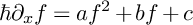
, and consider the Liouville transformation
$x_0$
, and consider the Liouville transformation
 $$ \begin{align} z = \Phi (x) {\mathrel{\mathop:}=} \int\nolimits_{x_0}^x \sqrt{ {{D}}_0 (t) } {\mathrm{d}}{t}. \end{align} $$
Suppose that $x_0$
has a neighborhood
$x_0$
has a neighborhood $\mathsf{W} \subset \mathsf{X}$
which is mapped by
$\mathsf{W} \subset \mathsf{X}$
which is mapped by $\Phi $
to a horizontal strip
$\Phi $
to a horizontal strip $\mathsf{H} = {\left \{ z ~\big |~ -r < {\operatorname {Im}} (z) < r \right \}}$
of some width
$\mathsf{H} = {\left \{ z ~\big |~ -r < {\operatorname {Im}} (z) < r \right \}}$
of some width $r> 0$
. Suppose furthermore that the
$r> 0$
. Suppose furthermore that the $\hbar $
-polynomial coefficients
$\hbar $
-polynomial coefficients $a_k, b_k, c_k$
of
$a_k, b_k, c_k$
of $a,b,c$
are bounded on
$a,b,c$
are bounded on $\mathsf{W}$
by
$\mathsf{W}$
by $\sqrt {{ {D}}_0}$
. Then, under these assumptions, the main results of this paper can be summarized as follows.
$\sqrt {{ {D}}_0}$
. Then, under these assumptions, the main results of this paper can be summarized as follows.
Theorem 1.1. The Riccati equation (1) has a pair of canonical exact solutions $f_{\pm }$
near
$f_{\pm }$
near $x_0 \in \mathsf{X}$
which are asymptotic to the formal solutions
$x_0 \in \mathsf{X}$
which are asymptotic to the formal solutions $\hat {f}_{\pm }$
as
$\hat {f}_{\pm }$
as $\hbar \to 0$
in the right half-plane. Namely, there is a neighborhood
$\hbar \to 0$
in the right half-plane. Namely, there is a neighborhood $\mathsf{U}_0 \subset \mathsf{X}$
of
$\mathsf{U}_0 \subset \mathsf{X}$
of $x_0$
and a sectorial subdomain
$x_0$
and a sectorial subdomain $\mathsf{S}_0 \subset \mathsf{S}$
with the same opening
$\mathsf{S}_0 \subset \mathsf{S}$
with the same opening $\mathrm{A}$
such that the Riccati equation (1) has a unique pair of holomorphic solutions
$\mathrm{A}$
such that the Riccati equation (1) has a unique pair of holomorphic solutions $f_{\pm }$
on
$f_{\pm }$
on $\mathsf{U}_0 \times \mathsf{S}_0$
which are Gevrey asymptotic to
$\mathsf{U}_0 \times \mathsf{S}_0$
which are Gevrey asymptotic to $\hat {f}_{\pm }$
as
$\hat {f}_{\pm }$
as $\hbar \to 0$
along the closed arc
$\hbar \to 0$
along the closed arc $\bar {\mathsf{A}}$
uniformly for all
$\bar {\mathsf{A}}$
uniformly for all $x \in \mathsf{U}_0$
:
$x \in \mathsf{U}_0$
:
 $$ \begin{align} f_{\pm} \simeq \hat{f}_{\pm} \qquad\qquad \text{as } \hbar \to 0 \text{ along } \bar{\mathsf{A}}, \text{ unif. } \forall x \in \mathsf{U}_0. \end{align} $$
Moreover, $f_{\pm }$
is the uniform Borel resummation of the formal solution
$f_{\pm }$
is the uniform Borel resummation of the formal solution $\hat {f}_{\pm }$
:
$\hat {f}_{\pm }$
:
 $$ \begin{align} f_{\pm} = \mathcal{S} \big[ \, \hat {f}_{\pm} \, \big]. \end{align} $$
This is a special case of Theorems 5.1 and 5.2, which are the two main results of this paper.
1.3 Discussion and method
We construct the canonical exact solutions $f_{\pm }$
by employing relatively basic and classical techniques from complex analysis which form the basis for the more modern and sophisticated theory of resurgent asymptotic analysis. Namely, we use the Borel–Laplace method, also known as the theory of Borel–Laplace summability. We stress that the Borel–Laplace method is nothing other than the theory of Laplace transforms, written in slightly different variables, echoing the words of Sokal [Reference Sokal17]. As such, we have tried to keep our presentation very hands-on and self-contained, so the knowledge of basic complex analysis should be sufficient to follow.
$f_{\pm }$
by employing relatively basic and classical techniques from complex analysis which form the basis for the more modern and sophisticated theory of resurgent asymptotic analysis. Namely, we use the Borel–Laplace method, also known as the theory of Borel–Laplace summability. We stress that the Borel–Laplace method is nothing other than the theory of Laplace transforms, written in slightly different variables, echoing the words of Sokal [Reference Sokal17]. As such, we have tried to keep our presentation very hands-on and self-contained, so the knowledge of basic complex analysis should be sufficient to follow.
An additional significant benefit of our approach is that we obtain uniqueness of the solution in the same sector where the initial data are specified. This feature does not hold for other less explicit approaches, such as, e.g., [Reference Wasow21, Theorem 26.1] where an existence theorem is proved only on a smaller subsector and there is no hope of uniqueness.
Finally, we want to take the opportunity to acknowledge the unpublished work of Koike and Schäfke on the Borel summability of WKB solutions of Schrödinger equations with polynomial potentials. See [Reference Takei19, §3.1] for a brief account of their work. Their ideas (which were kindly explained to the author in a private communication from Kohei Iwaki) provided the initial inspiration for the more general strategy of the proof pursued in this article.
2 Singularly perturbed Riccati equations
2.1 Background assumptions
Throughout the paper, we fix a complex plane ${\mathbb {C}}_x$
with coordinate x and another complex plane
${\mathbb {C}}_x$
with coordinate x and another complex plane ${\mathbb {C}}_{\hbar }$
with coordinate
${\mathbb {C}}_{\hbar }$
with coordinate $\hbar $
. Let
$\hbar $
. Let $\mathsf{X}$
be a domain in
$\mathsf{X}$
be a domain in ${\mathbb {C}}_x$
or indeed a coordinate chart on a Riemann surface. Let
${\mathbb {C}}_x$
or indeed a coordinate chart on a Riemann surface. Let $\mathsf{S} \subset {\mathbb {C}}_{\hbar }$
be a sectorial domain at the origin with opening arc
$\mathsf{S} \subset {\mathbb {C}}_{\hbar }$
be a sectorial domain at the origin with opening arc $\mathsf{A}$
. We assume that
$\mathsf{A}$
. We assume that $0 < |\mathsf{A}| \leq 2\pi $
.
$0 < |\mathsf{A}| \leq 2\pi $
.
Consider the Riccati equation
 $$ \begin{align} \hbar \partial_x f = a f^2 + b f + c \end{align} $$
whose coefficients $a,b,c$
are holomorphic functions of
$a,b,c$
are holomorphic functions of $(x,\hbar ) \in \mathsf{X} \times \mathsf{S}$
admitting locally uniform asymptotic expansions with holomorphic coefficients as
$(x,\hbar ) \in \mathsf{X} \times \mathsf{S}$
admitting locally uniform asymptotic expansions with holomorphic coefficients as $\hbar \to 0$
along
$\hbar \to 0$
along $\mathsf{A}$
:
$\mathsf{A}$
:
 $$ \begin{align} \begin{aligned} a (x, \hbar) &\sim \hat{a} (x, \hbar) {\mathrel{\mathop:}=} \sum_{n = 0}^{\infty} a_n (x) \hbar^n {,}\\ b (x, \hbar) &\sim \hat{b} (x, \hbar) {\mathrel{\mathop:}=} \sum_{n = 0}^{\infty} b_n (x) \hbar^n {,} \\ c (x, \hbar) &\sim \hat{c} (x, \hbar) {\mathrel{\mathop:}=} \sum_{n = 0}^{\infty} c_n (x) \hbar^n. \end{aligned} \qquad\qquad \text{as } \hbar \to 0 \text{ along } \mathsf{A}, \text{ loc.unif. } \forall x \in \mathsf{X} {,} \end{align} $$
The main problem we pose in this article is to find canonical exact solutions of the Riccati equation (5) in the following sense.
Definition 2.1. Fix any phase $\theta \in \mathsf{A}$
. A local
$\theta \in \mathsf{A}$
. A local $\theta $
-exact solution of the Riccati equation (5) near a point
$\theta $
-exact solution of the Riccati equation (5) near a point $x_0 \in \mathsf{X}$
is a holomorphic solution
$x_0 \in \mathsf{X}$
is a holomorphic solution $f = f(x,\hbar )$
, defined on a domain
$f = f(x,\hbar )$
, defined on a domain $\mathsf{U}_0 \times \mathsf{S}_0$
where
$\mathsf{U}_0 \times \mathsf{S}_0$
where $\mathsf{U}_0 \subset \mathsf{X}$
is a neighborhood of
$\mathsf{U}_0 \subset \mathsf{X}$
is a neighborhood of $x_0$
and
$x_0$
and $\mathsf{S}_0 \subset \mathsf{S}$
is a sectorial subdomain with opening
$\mathsf{S}_0 \subset \mathsf{S}$
is a sectorial subdomain with opening $\mathsf{A}_0 \subset \mathsf{A}$
containing
$\mathsf{A}_0 \subset \mathsf{A}$
containing $\theta $
, such that f admits an asymptotic expansion with holomorphic coefficients as
$\theta $
, such that f admits an asymptotic expansion with holomorphic coefficients as $\hbar \to 0$
along
$\hbar \to 0$
along $\mathsf{A}_0$
uniformly for all
$\mathsf{A}_0$
uniformly for all $x \in \mathsf{U}_0$
.
$x \in \mathsf{U}_0$
.
A $\theta $
-exact solution on a domain
$\theta $
-exact solution on a domain $\mathsf{U} \subset \mathsf{X}$
is a holomorphic solution
$\mathsf{U} \subset \mathsf{X}$
is a holomorphic solution $f = f(x,\hbar )$
which is a local
$f = f(x,\hbar )$
which is a local $\theta $
-exact solution near every point in
$\theta $
-exact solution near every point in $\mathsf{U}$
. That is, f is a holomorphic solution defined on a domain
$\mathsf{U}$
. That is, f is a holomorphic solution defined on a domain ${\mathbb {U}} \subset \mathsf{U} \times \mathsf{S}$
with the following property: for every
${\mathbb {U}} \subset \mathsf{U} \times \mathsf{S}$
with the following property: for every $x_0 \in \mathsf{X}$
, there is a domain neighborhood
$x_0 \in \mathsf{X}$
, there is a domain neighborhood $\mathsf{U}_0 \subset \mathsf{U}$
of
$\mathsf{U}_0 \subset \mathsf{U}$
of $x_0$
and a sectorial domain
$x_0$
and a sectorial domain $\mathsf{S}_0 \subset \mathsf{S}$
with opening
$\mathsf{S}_0 \subset \mathsf{S}$
with opening $\mathsf{A}_0 \subset \mathsf{A}$
containing
$\mathsf{A}_0 \subset \mathsf{A}$
containing $\theta $
such that f admits an asymptotic expansion with holomorphic coefficients as
$\theta $
such that f admits an asymptotic expansion with holomorphic coefficients as $\hbar \to 0$
along
$\hbar \to 0$
along $\mathsf{A}_0$
uniformly for all
$\mathsf{A}_0$
uniformly for all $x \in \mathsf{U}_0$
.
$x \in \mathsf{U}_0$
.
2.2 Examples
The following is a list, included here for illustrative purposes only, containing a few explicit examples of Riccati equations to which the main results in this paper can be applied.
The most typical situation is one where the coefficients $a,b,c$
of the Riccati equation (5) are polynomials in
$a,b,c$
of the Riccati equation (5) are polynomials in $\hbar $
with coefficients which are rational functions of x. In this case,
$\hbar $
with coefficients which are rational functions of x. In this case, $\mathsf{X}$
is the complement of the poles in
$\mathsf{X}$
is the complement of the poles in ${\mathbb {C}}_x$
, and the sectorial domain
${\mathbb {C}}_x$
, and the sectorial domain $\mathsf{S}$
can be taken to be the whole open right half-plane
$\mathsf{S}$
can be taken to be the whole open right half-plane ${\left \{ {\operatorname {Re}} (\hbar )> 0 \right \}}$
. The simplest example is
${\left \{ {\operatorname {Re}} (\hbar )> 0 \right \}}$
. The simplest example is
-
(1) ${\hbar \partial _x f = f^2 - x}$
.
${\hbar \partial _x f = f^2 - x}$
.

This Riccati equation is examined in great detail in §6.2. It arises in the exact WKB analysis of the Airy equation $\hbar ^{2} \partial _{x}^{2} \psi (x, \hbar ) = x \psi (x, \hbar )$
(see [Reference Nikolaev12]). In this case,
$\hbar ^{2} \partial _{x}^{2} \psi (x, \hbar ) = x \psi (x, \hbar )$
(see [Reference Nikolaev12]). In this case, $\mathsf{X} = {\mathbb {C}}_x$
and the sectorial domain
$\mathsf{X} = {\mathbb {C}}_x$
and the sectorial domain $\mathsf{S}$
is the open right half-plane
$\mathsf{S}$
is the open right half-plane ${\left \{ {\operatorname {Re}} (\hbar )> 0 \right \}}$
. If
${\left \{ {\operatorname {Re}} (\hbar )> 0 \right \}}$
. If $\mathsf{U}$
is any of the three sectorial domains in
$\mathsf{U}$
is any of the three sectorial domains in ${\mathbb {C}}_x$
given by
${\mathbb {C}}_x$
given by ${\left \{ 0 < \arg (x) < +4\pi /3 \right \}}$
, or
${\left \{ 0 < \arg (x) < +4\pi /3 \right \}}$
, or ${\left \{ +2\pi /3 < \arg (x) < +2\pi \right \}}$
, or
${\left \{ +2\pi /3 < \arg (x) < +2\pi \right \}}$
, or ${\left \{ -2\pi /3 < \arg (x) < +2\pi /3 \right \}}$
, then on each of these domains, the main existence and uniqueness result in this paper produces a pair of canonical exact solutions. More generally,
${\left \{ -2\pi /3 < \arg (x) < +2\pi /3 \right \}}$
, then on each of these domains, the main existence and uniqueness result in this paper produces a pair of canonical exact solutions. More generally,
-
(2)
${\hbar \partial _x f = f^2 + q(x)}$
,

where $q(x)$
is any polynomial or a rational function with poles of order
$q(x)$
is any polynomial or a rational function with poles of order $2$
or higher. In this case,
$2$
or higher. In this case, $\mathsf{S}$
can again be arranged to be the right half-plane, and
$\mathsf{S}$
can again be arranged to be the right half-plane, and $\mathsf{U}$
is a sectorial domain near a pole of
$\mathsf{U}$
is a sectorial domain near a pole of $q(x)$
of order
$q(x)$
of order $2$
or higher.
$2$
or higher.
Many Riccati equations arise from the WKB analysis of classical second-order differential equation. For example, the following Riccati equation appears in the WKB analysis of the Gauss hypergeometric equation:
-
(3)
${\hbar \partial _x f = f^2 + \frac {\gamma - (\alpha + \beta + 1) x}{x(x-1)} f + \frac {\alpha \beta }{x (x-1)}}$
for any
$\alpha , \beta , \gamma \in {\mathbb {C}}^{\ast }$
.


Riccati equations also arise in the analysis of singularly perturbed second-order systems. For example, the Riccati equation
-
(4)
${\hbar \partial _x f = \hbar f^2 + (1-x) f + x \hbar }$

arises in the analysis of the system $\hbar \partial _{x} \psi + \begin {bmatrix} 1 & - \hbar \\ x\hbar & x\end {bmatrix} \psi = 0$
. See [Reference Nikolaev13].
$\hbar \partial _{x} \psi + \begin {bmatrix} 1 & - \hbar \\ x\hbar & x\end {bmatrix} \psi = 0$
. See [Reference Nikolaev13].
Our methods also apply to the following nontrivial deformation of example (1):
-
(5)
${\hbar \partial _x f = f^2 - x + x { {E}} (x, \hbar ) \quad \text {where} \quad { {E}} (x, \hbar ) {\mathrel {\mathop :}=} \int _0^{+\infty } \frac {e^{- \xi /\hbar }}{x + \xi } {\mathrm {d}}{\xi }}$
.

The sectorial domain $\mathsf{S}$
in this case is the open right half-plane. The function
$\mathsf{S}$
in this case is the open right half-plane. The function ${ {E}} $
is holomorphic in
${ {E}} $
is holomorphic in $\hbar \in \mathsf{S}$
, and it admits a locally uniform asymptotic expansion as
$\hbar \in \mathsf{S}$
, and it admits a locally uniform asymptotic expansion as $\hbar \to 0$
in the right half-plane. Notice, however, that
$\hbar \to 0$
in the right half-plane. Notice, however, that ${ {E}} $
is not holomorphic at
${ {E}} $
is not holomorphic at $\hbar = 0$
, and it also has nonisolated singularities along the negative real axis in
$\hbar = 0$
, and it also has nonisolated singularities along the negative real axis in ${\mathbb {C}}_x$
. Nevertheless, if
${\mathbb {C}}_x$
. Nevertheless, if $\mathsf{U}$
is the domain given by
$\mathsf{U}$
is the domain given by ${\left \{ -2\pi /3 < \arg (x) < +2\pi /3 \right \}}$
or by
${\left \{ -2\pi /3 < \arg (x) < +2\pi /3 \right \}}$
or by ${\left \{ 0 < \arg (x) < +\pi \right \}}$
or
${\left \{ 0 < \arg (x) < +\pi \right \}}$
or ${\left \{ +\pi < \arg (x) < +2\pi \right \}}$
, then our method yields canonical exact solutions on
${\left \{ +\pi < \arg (x) < +2\pi \right \}}$
, then our method yields canonical exact solutions on $\mathsf{U}$
.
$\mathsf{U}$
.
3 Formal perturbation theory
In this section, we analyze the Riccati equation from a purely formal perspective whereby we ignore all analytic considerations in the $\hbar $
-variable.
$\hbar $
-variable.
Thus, we consider the formal Riccati equation
 $$ \begin{align} \hbar \partial_x \hat{f} = \hat{a} \hat{f}^2 + \hat{b} \hat{f} + \hat{c}, \end{align} $$
where $\hat {a}, \hat {b}, \hat {c}$
are arbitrary formal power series in
$\hat {a}, \hat {b}, \hat {c}$
are arbitrary formal power series in $\hbar $
with holomorphic coefficients on some domain
$\hbar $
with holomorphic coefficients on some domain $\mathsf{X}$
in
$\mathsf{X}$
in ${\mathbb {C}}_x$
. By definition, a formal solution of (7) on a domain
${\mathbb {C}}_x$
. By definition, a formal solution of (7) on a domain $\mathsf{U} \subset \mathsf{X}$
is any formal power series with holomorphic coefficients
$\mathsf{U} \subset \mathsf{X}$
is any formal power series with holomorphic coefficients $\hat {f} = \hat {f} (x, \hbar )$
that satisfies the formal equation (7).
$\hat {f} = \hat {f} (x, \hbar )$
that satisfies the formal equation (7).
3.1 Leading-order solutions
Consider the leading-order equation corresponding to (7):
 $$ \begin{align} a_0 f_0^2 + b_0 f_0 + c_0 = 0. \end{align} $$
It is a quadratic equation in the unknown variable $f_0$
, and we refer to its solutions as leading-order solutions of the Riccati equation. Generically, they are locally holomorphic, but may have poles and branch-point singularities.
$f_0$
, and we refer to its solutions as leading-order solutions of the Riccati equation. Generically, they are locally holomorphic, but may have poles and branch-point singularities.
The discriminant of (8),
 $$ \begin{align} {{D}}_0 {\mathrel{\mathop:}=} b_0^2 - 4 a_0 c_0, \end{align} $$
which we call the leading-order discriminant of the Riccati equation, is a holomorphic function on $\mathsf{X}$
. We always assume that
$\mathsf{X}$
. We always assume that ${ {D}}_0$
is not identically zero. The zeros of
${ {D}}_0$
is not identically zero. The zeros of ${ {D}}_0$
are called turning points of the Riccati equation, and all other points in
${ {D}}_0$
are called turning points of the Riccati equation, and all other points in $\mathsf{X}$
are called regular points. Locally, away from turning points, there is at least one holomorphic leading-order solution. For reference, we state the following elementary lemma.
$\mathsf{X}$
are called regular points. Locally, away from turning points, there is at least one holomorphic leading-order solution. For reference, we state the following elementary lemma.
Lemma 3.1 (Holomorphic leading-order solutions).
Let $\mathsf{U} \subset \mathsf{X}$
be any domain free of turning points such that a univalued square-root branch
$\mathsf{U} \subset \mathsf{X}$
be any domain free of turning points such that a univalued square-root branch $\sqrt { { {D}}_0 }$
of
$\sqrt { { {D}}_0 }$
of ${ {D}}_0$
can be chosen on
${ {D}}_0$
can be chosen on $\mathsf{U}$
. Then the leading-order equation (8) has at least one holomorphic solution on
$\mathsf{U}$
. Then the leading-order equation (8) has at least one holomorphic solution on $\mathsf{U}$
. In addition, if
$\mathsf{U}$
. In addition, if $a_0$
is nonvanishing on
$a_0$
is nonvanishing on $\mathsf{U}$
, then (8) has two holomorphic solutions. Moreover, any holomorphic solution is bounded on
$\mathsf{U}$
, then (8) has two holomorphic solutions. Moreover, any holomorphic solution is bounded on $\mathsf{U}$
whenever the coefficients
$\mathsf{U}$
whenever the coefficients $a_0, b_0, c_0$
are bounded by
$a_0, b_0, c_0$
are bounded by $\sqrt {{ {D}}_0}$
on
$\sqrt {{ {D}}_0}$
on $\mathsf{U}$
.
$\mathsf{U}$
.
We will always label the leading-order solutions as follows:
 $$ \begin{align} f_0^{\pm} {\mathrel{\mathop:}=} \frac{-b_0 \pm \sqrt{{{D}}_0}}{2 a_0} &\qquad\text{if } a_0 \not\equiv 0, \end{align} $$
 $$ \begin{align} f_0^+ {\mathrel{\mathop:}=} - c_0 / b_0 &\qquad\text{if } a_0 \equiv 0.\\[-9pt]\nonumber\end{align} $$
This choice of labels yields the following relations:
 $$ \begin{align} \pm \sqrt{{{D}}_0} = 2a_0 f_0^{\pm} + b_0 \qquad \text{and} \qquad \sqrt{{{D}}_0} = a_0 \big( f_0^+ - f_0^- \big).\\[-15pt]\nonumber \end{align} $$
Thus, if $a_0$
is nonvanishing, then both
$a_0$
is nonvanishing, then both $f_0^{\pm }$
from (10a) are holomorphic functions on
$f_0^{\pm }$
from (10a) are holomorphic functions on $\mathsf{U}$
. If
$\mathsf{U}$
. If $a_0$
has zeros in
$a_0$
has zeros in $\mathsf{U}$
, then
$\mathsf{U}$
, then $f_0^+$
from (10a) remains holomorphic on
$f_0^+$
from (10a) remains holomorphic on $\mathsf{U}$
, but
$\mathsf{U}$
, but $f_0^-$
has poles where
$f_0^-$
has poles where $a_0$
has zeros. If
$a_0$
has zeros. If $a_0 \equiv 0$
, then
$a_0 \equiv 0$
, then $f_0^+$
from (10b) is a holomorphic function on
$f_0^+$
from (10b) is a holomorphic function on $\mathsf{U}$
.
$\mathsf{U}$
.
3.2 Existence and uniqueness of formal solutions
The following elementary theorem says that a formal Riccati equation (7) always has at least one local solution away from turning points, and it is uniquely specified in the leading-order.
Theorem 3.1 (Formal existence and uniqueness theorem).
Consider the formal Riccati equation (7). Assume that its leading-order discriminant ${ {D}}_0$
is not identically zero. Let
${ {D}}_0$
is not identically zero. Let $\mathsf{U} \subset \mathsf{X}$
be a domain free of turning points that supports a univalued square-root branch
$\mathsf{U} \subset \mathsf{X}$
be a domain free of turning points that supports a univalued square-root branch $\sqrt {{ {D}}_0}$
.
$\sqrt {{ {D}}_0}$
.
-
(1) If
$a_0 \equiv 0$
, then (7) has a unique formal solution
$\hat {f}_+$
on
$\mathsf{U}$
. Its leading-order term is
$f_0^+$
from (10b). -
(2) If
$a_0 \not \equiv 0$
and nonvanishing on
$\mathsf{U}$
, then (7) has exactly two distinct formal solutions
$\hat {f}_{\pm }$
on
$\mathsf{U}$
. Their leading-order terms
$f^{\pm }_0$
are given by (10a). -
(3) If
$a_0 \not \equiv 0$
but has zeros in
$\mathsf{U}$
, then (7) has a unique formal solution
$\hat {f}_+$
on
$\mathsf{U}$
. Its leading-order term
$f_0^+$
is the unique holomorphic leading-order solution on
$\mathsf{U}$
given by (10a).


Moreover, the coefficients $f_k^{\pm }$
of
$f_k^{\pm }$
of $\hat {f}_{\pm }$
for
$\hat {f}_{\pm }$
for $k \geq 1$
are given by the following recursive formula:
$k \geq 1$
are given by the following recursive formula:
 $$ \begin{align} f_k^{\pm} = \pm \frac{1}{\sqrt{ {{D}}_0 }} \partial_x f_{k-1}^{\pm} \mp \frac{1}{\sqrt{ {{D}}_0 }} \left(\sum_{k_1 + k_2 + k_3 = k}^{k_2, k_3 \neq k} a_{k_1} f_{k_2}^{\pm} f_{k_3}^{\pm} + \sum_{k_1 + k_2 = k}^{k_2 \neq k} b_{k_1} f_{k_2}^{\pm} + c_k \right).\\[-9pt]\nonumber \end{align} $$
Proof. We expand the formal Riccati equation (7) order-by-order in $\hbar $
:
$\hbar $
:
 $$ \begin{align} \hbar^0 ~\big|~ ~ & 0 = a_0 f_0^2 + b_0 f_0 + c_0;\phantom{+ b_1 f_0 + c_1;+ b_1 f_0 + c_1 a_2 f_0^2 . .b_1 f_1 + b_2 f_0 + c_2;} \end{align} $$
 $$ \begin{align} \hbar^1 ~\big|~ ~ &\partial_x f_0 = (2a_0 f_0 + b_0) f_1 + a_1 f_0^2 + b_1 f_0 + c_1;\phantom{+ a_2 f_0^2 . .b_1 f_1 + b_2 f_0 + c_2;} \end{align} $$
 $$ \begin{align} \hbar^2 ~\big|~ ~ &\partial_x f_1 = (2a_0 f_0 + b_0) f_2 + a_0 f_1^2 + 2 a_1 f_0 f_1 + a_2 f_0^2 + b_1 f_1 + b_2 f_0 + c_2; \end{align} $$
 $$ \begin{align} \nonumber \vdots \phantom{~~\big|~ ~}\nonumber \\ \hbar^k ~\big|~ ~ &\partial_x f_{k-1} = (2a_0 f_0 + b_0) f_k + \sum_{k_1 + k_2 + k_3 = k}^{k_2, k_3 \neq k} a_{k_1} f_{k_2} f_{k_3} + \sum_{k_1 + k_2 = k}^{k_2 \neq k} b_{k_1} f_{k_2} + c_k.\\ \nonumber \vdots \phantom{~~\big|~ ~} \end{align} $$
Observe that these are no longer differential equations because the derivative term at each order depends only on the solutions from previous orders. If we fix a leading-order solution $f_0^{\pm }$
, then the expression
$f_0^{\pm }$
, then the expression $(2 a_0 f_0^{\pm } + b_0)$
, appearing as a factor in front of
$(2 a_0 f_0^{\pm } + b_0)$
, appearing as a factor in front of $f^{\pm }_k$
in each equation (16), is simply
$f^{\pm }_k$
in each equation (16), is simply $\pm \sqrt {{ {D}}_0}$
. From the assumption that
$\pm \sqrt {{ {D}}_0}$
. From the assumption that ${ {D}}_0 \not \equiv 0$
, it follows that at each order in
${ {D}}_0 \not \equiv 0$
, it follows that at each order in $\hbar $
, we can uniquely solve for
$\hbar $
, we can uniquely solve for $f_k^{\pm }$
. This establishes the formula (12), from which the other statements readily follow.
$f_k^{\pm }$
. This establishes the formula (12), from which the other statements readily follow.
Remark 3.1. In Theorem 3.1(3), the Riccati equation (7) also has a singular formal solution $\hat {f}_-$
on
$\hat {f}_-$
on $\mathsf{U}$
whose leading-order term is the singular leading-order solution
$\mathsf{U}$
whose leading-order term is the singular leading-order solution $f_0^-$
on
$f_0^-$
on $\mathsf{U}$
. The singularities of the coefficients of
$\mathsf{U}$
. The singularities of the coefficients of $\hat {f}_-$
are poles occurring at the zeros of
$\hat {f}_-$
are poles occurring at the zeros of $a_0$
. We will examine in more detail the singularities of formal (and exact) solutions in a forthcoming paper.
$a_0$
. We will examine in more detail the singularities of formal (and exact) solutions in a forthcoming paper.
Remark 3.2 (Formal discriminant).
Since in the generic situation the Riccati equation has precisely two formal solutions $\hat {f}_+, \hat {f}_-$
, we can introduce a notion of discriminant for the Riccati equation analogous to the discriminant of a quadratic equation by simply mimicking the formula.
$\hat {f}_+, \hat {f}_-$
, we can introduce a notion of discriminant for the Riccati equation analogous to the discriminant of a quadratic equation by simply mimicking the formula.
Thus, let $\mathsf{U} \subset \mathsf{X}$
be a domain free of turning points that supports a univalued square-root branch
$\mathsf{U} \subset \mathsf{X}$
be a domain free of turning points that supports a univalued square-root branch $\sqrt {{ {D}}_0}$
, and suppose that
$\sqrt {{ {D}}_0}$
, and suppose that $a_0$
is nonvanishing on
$a_0$
is nonvanishing on $\mathsf{U}$
. We define the formal discriminant of the Riccati equation (7) by the following formula:
$\mathsf{U}$
. We define the formal discriminant of the Riccati equation (7) by the following formula:
 $$ \begin{align} \hat{{{D}}} {\mathrel{\mathop:}=} \hat{a}^2 \big( \hat{f}_+ - \hat{f}_- \big) \big( \hat{f}_- - \hat{f}_+ \big). \end{align} $$
It is a formal power series with holomorphic coefficients on $\mathsf{U}$
, and its leading-order term is precisely the leading-order discriminant
$\mathsf{U}$
, and its leading-order term is precisely the leading-order discriminant ${ {D}}_0$
. This quantity plays an important role in addressing global questions in the WKB analysis that will be studied elsewhere.
${ {D}}_0$
. This quantity plays an important role in addressing global questions in the WKB analysis that will be studied elsewhere.
3.3 Gevrey regularity of formal solutions
In this subsection, we prove the following general result about the regularity of formal solutions, which generalizes Proposition A.1.1 in [Reference Aoki, Kawai and Takei1, p. 19] (see also [Reference Voros20, p. 252]), where it is assumed that $\hat {a} = -1, \hat {b} = 0$
, and
$\hat {a} = -1, \hat {b} = 0$
, and $\hat {c}$
is an entire holomorphic function of x only (i.e.,
$\hat {c}$
is an entire holomorphic function of x only (i.e., $\hat {c} (x, \hbar ) = c_0 (x)$
).
$\hat {c} (x, \hbar ) = c_0 (x)$
).
Proposition 3.1 (Local Gevrey regularity of formal solutions).
Consider a formal Riccati equation (7) on $\mathsf{X}$
with leading-order discriminant
$\mathsf{X}$
with leading-order discriminant ${ {D}}_0 \not \equiv 0$
. Let
${ {D}}_0 \not \equiv 0$
. Let $\mathsf{U} \subset \mathsf{X}$
be any domain free of turning points that supports a univalued square-root branch
$\mathsf{U} \subset \mathsf{X}$
be any domain free of turning points that supports a univalued square-root branch $\sqrt {{ {D}}_0}$
, and let
$\sqrt {{ {D}}_0}$
, and let $\hat {f}$
be a formal solution on
$\hat {f}$
be a formal solution on $\mathsf{U}$
. If the coefficients
$\mathsf{U}$
. If the coefficients $\hat {a},\hat {b},\hat {c}$
are locally uniformly Gevrey series on
$\hat {a},\hat {b},\hat {c}$
are locally uniformly Gevrey series on $\mathsf{U}$
, then so is
$\mathsf{U}$
, then so is $\hat {f}$
. In particular, the formal Borel transform
$\hat {f}$
. In particular, the formal Borel transform $\hat {\phi } (x, \xi ) {\mathrel {\mathop :}=} \hat {{\mathfrak {B}}} [ \, \hat {f} \, ] (x, \xi )$
of
$\hat {\phi } (x, \xi ) {\mathrel {\mathop :}=} \hat {{\mathfrak {B}}} [ \, \hat {f} \, ] (x, \xi )$
of $\hat {f}$
is a locally uniformly convergent power series in
$\hat {f}$
is a locally uniformly convergent power series in $\xi $
.
$\xi $
.
Concretely, Proposition 3.1 says that if the coefficients $a_k, b_k, c_k$
of the power series
$a_k, b_k, c_k$
of the power series $\hat {a},\hat {b},\hat {c}$
grow at most like
$\hat {a},\hat {b},\hat {c}$
grow at most like $k!$
, then the coefficients
$k!$
, then the coefficients $f_k$
of any formal solution
$f_k$
of any formal solution $\hat {f}$
likewise grow at most like
$\hat {f}$
likewise grow at most like $k!$
. This is made precise in the following corollary.
$k!$
. This is made precise in the following corollary.
Corollary 3.1 (At most factorial growth).
Consider a formal Riccati equation (7) on $\mathsf{X}$
with leading-order discriminant
$\mathsf{X}$
with leading-order discriminant ${ {D}}_0 \not \equiv 0$
. Let
${ {D}}_0 \not \equiv 0$
. Let $\mathsf{U} \subset \mathsf{X}$
be any domain free of turning points that supports a univalued square-root branch
$\mathsf{U} \subset \mathsf{X}$
be any domain free of turning points that supports a univalued square-root branch $\sqrt {{ {D}}_0}$
, and let
$\sqrt {{ {D}}_0}$
, and let $\hat {f}$
be a formal solution on
$\hat {f}$
be a formal solution on $\mathsf{U}$
. Take any pair of nested compactly contained subsets
$\mathsf{U}$
. Take any pair of nested compactly contained subsets $\mathsf{U}_0 \Subset \mathsf{U}_1 \Subset \mathsf{U}$
, and suppose that there are real constants
$\mathsf{U}_0 \Subset \mathsf{U}_1 \Subset \mathsf{U}$
, and suppose that there are real constants ${ {A}}, { {B}}> 0$
such that
${ {A}}, { {B}}> 0$
such that
 $$ \begin{align} \big| a_k (x) \big|,\big| b_k (x) \big|, \big| c_k (x) \big| \leq {{A}} {{B}}^{k} k! \qquad\quad (\forall k \geq 0, \forall x \in \mathsf{U}_1). \end{align} $$
Then there are real constants ${ {C}}, { {M}}> 0$
such that
${ {C}}, { {M}}> 0$
such that
 $$ \begin{align} \big| f_k (x) \big| \leq {{C}} {{M}}^{k} k! \qquad\qquad\qquad (\forall k \geq 0, \forall x \in \mathsf{U}_0). \end{align} $$
Proof of Proposition 3.1
Let ${\mathbb {D}}_{{ {R}}} \subset \mathsf{U}$
be any sufficiently small disk of some radius
${\mathbb {D}}_{{ {R}}} \subset \mathsf{U}$
be any sufficiently small disk of some radius ${ {R}}> 0$
on which
${ {R}}> 0$
on which $\hat {a}, \hat {b}, \hat {c}$
are uniformly Gevrey and
$\hat {a}, \hat {b}, \hat {c}$
are uniformly Gevrey and $\sqrt {{ {D}}_0}$
is bounded both above and below by a nonzero constant. Thus, there are real constants
$\sqrt {{ {D}}_0}$
is bounded both above and below by a nonzero constant. Thus, there are real constants ${ {A}}, { {B}}> 0$
, which give the following uniform bounds:
${ {A}}, { {B}}> 0$
, which give the following uniform bounds:
 $$ \begin{align} \big| a_k (x) \big|, \big| b_k (x) \big|, \big| c_k (x) \big| \leq {{A}} {{B}}^{k} k! \qquad \text{and}\qquad {{A}}^{-1} \leq \big| \sqrt{{{D}}_0 (x)} \big| \leq {{A}} \end{align} $$
for all integers $k \geq 0$
and all
$k \geq 0$
and all $x \in {\mathbb {D}}_{{ {R}}}$
. It will be convenient for us to assume without loss of generality that
$x \in {\mathbb {D}}_{{ {R}}}$
. It will be convenient for us to assume without loss of generality that ${ {A}} \geq 3$
and
${ {A}} \geq 3$
and ${ {R}} < 1$
. We will prove that
${ {R}} < 1$
. We will prove that $\hat {f}$
is a uniformly Gevrey power series on any compactly contained subset of
$\hat {f}$
is a uniformly Gevrey power series on any compactly contained subset of ${\mathbb {D}}_{{ {R}}}$
. In fact, we will prove something a little bit stronger as follows. For any
${\mathbb {D}}_{{ {R}}}$
. In fact, we will prove something a little bit stronger as follows. For any $r \in (0, { {R}})$
, denote by
$r \in (0, { {R}})$
, denote by ${\mathbb {D}}_r \subset {\mathbb {D}}_{{ {R}}}$
the concentric subdisk of radius r. Then Proposition 3.1 follows from the following claim.
${\mathbb {D}}_r \subset {\mathbb {D}}_{{ {R}}}$
the concentric subdisk of radius r. Then Proposition 3.1 follows from the following claim.
Claim 3.1. There exist real constants ${ {C}}, { {M}}> 0$
such that, for any
${ {C}}, { {M}}> 0$
such that, for any $r \in (0,{ {R}})$
,
$r \in (0,{ {R}})$
,
 $$ \begin{align} \big| f_k (x) \big| \leq {{C}} {{M}}^k \delta^{-k} k! \end{align} $$
for all integers $k \geq 0$
and uniformly for all
$k \geq 0$
and uniformly for all $x \in {\mathbb {D}}_r$
, where
$x \in {\mathbb {D}}_r$
, where $\delta {\mathrel {\mathop :}=} { {R}} - r$
. (The constants
$\delta {\mathrel {\mathop :}=} { {R}} - r$
. (The constants ${ {C}}, { {M}}$
are independent of
${ {C}}, { {M}}$
are independent of $r, x, k$
, but may depend on
$r, x, k$
, but may depend on ${ {R}}, { {A}}, { {B}}$
.) In particular, for any
${ {R}}, { {A}}, { {B}}$
.) In particular, for any $r \in (0,{ {R}})$
, the power series
$r \in (0,{ {R}})$
, the power series $\hat {f}$
is Gevrey uniformly for all
$\hat {f}$
is Gevrey uniformly for all $x \in {\mathbb {D}}_r$
.
$x \in {\mathbb {D}}_r$
.
Proof. First, it is easy to find a constant ${ {C}}> 0$
(independent of r) such that
${ {C}}> 0$
(independent of r) such that
 $$ \begin{align} \big| f_0 (x) \big| \leq {{C}} \end{align} $$
uniformly for all $x \in {\mathbb {D}}_{{ {R}}}$
(see Lemma 3.1). Without loss of generality, assume that
$x \in {\mathbb {D}}_{{ {R}}}$
(see Lemma 3.1). Without loss of generality, assume that
 $$ \begin{align} {{C}} \geq {{A}} \geq 3. \end{align} $$
Then the bound (21) will be demonstrated in two main steps. First, we will recursively construct a sequence $({ {M}}_k)_{k=0}^{\infty }$
of positive real numbers such that, for all
$({ {M}}_k)_{k=0}^{\infty }$
of positive real numbers such that, for all $k \geq 0$
and all
$k \geq 0$
and all $r \in (0,{ {R}})$
, we have the following uniform bound for all
$r \in (0,{ {R}})$
, we have the following uniform bound for all $x \in {\mathbb {D}}_r$
:
$x \in {\mathbb {D}}_r$
:
 $$ \begin{align} \big| f_k (x) \big| \leq {{C}} {{M}}_k \delta^{-k} k!. \end{align} $$
Then we will show that there is a constant ${ {M}}> 0$
(independent of r) such that
${ {M}}> 0$
(independent of r) such that ${ {M}}_k \leq { {M}}^k$
for all k.
${ {M}}_k \leq { {M}}^k$
for all k.
Construction of $({ {M}}_k)_{k = 0}^{\infty }$
. The bound (24) for
$({ {M}}_k)_{k = 0}^{\infty }$
. The bound (24) for $k = 0$
is just the bound (22) if we put
$k = 0$
is just the bound (22) if we put ${ {M}}_0 {\mathrel {\mathop :}=} 1$
. Now, we use induction on k and formula (12). Assume that we have already constructed positive real numbers
${ {M}}_0 {\mathrel {\mathop :}=} 1$
. Now, we use induction on k and formula (12). Assume that we have already constructed positive real numbers ${ {M}}_0, \ldots , { {M}}_{k-1}$
such that, for all
${ {M}}_0, \ldots , { {M}}_{k-1}$
such that, for all $i = 0, \ldots , k-1$
, all
$i = 0, \ldots , k-1$
, all $r \in (0,{ {R}})$
, and all
$r \in (0,{ {R}})$
, and all $x \in {\mathbb {D}}_r$
, we have the bound
$x \in {\mathbb {D}}_r$
, we have the bound
 $$ \begin{align} \big| f_i (x) \big| \leq {{C}} {{M}}_i \delta^{-i} i!. \end{align} $$
In order to derive an estimate for $f_k$
, we first need to estimate the derivative term
$f_k$
, we first need to estimate the derivative term $\partial _x f_{k-1}$
, for which we use Cauchy estimates as follows.
$\partial _x f_{k-1}$
, for which we use Cauchy estimates as follows.
Sub-Claim. For all $r \in (0,{ {R}})$
and all
$r \in (0,{ {R}})$
and all $x \in {\mathbb {D}}_r$
,
$x \in {\mathbb {D}}_r$
,
 $$ \begin{align} \big| \partial_x f_{k-1} (x) \big| \leq {{C}}^2 {{M}}_{k-1} \delta^{-k} k!. \end{align} $$
Proof of Sub-Claim
For every $r \in (0,{ {R}})$
, define
$r \in (0,{ {R}})$
, define
 $$ \begin{align*} \delta_k {\mathrel{\mathop:}=} \delta \frac{k}{k+1} \qquad\text{and}\qquad r_k {\mathrel{\mathop:}=} {{R}} - \delta_k. \end{align*} $$
Inequality (25) holds in particular for $i = k-1$
,
$i = k-1$
, $r = r_k$
. So for all
$r = r_k$
. So for all $x \in {\mathbb {D}}_{r_k}$
, we find
$x \in {\mathbb {D}}_{r_k}$
, we find
 $$ \begin{align*} \big| f_{k-1} (x) \big|\leq {{C}} {{M}}_{k-1} \delta_k^{1-k} (k-1)! \leq {{C}}^2 {{M}}_{k-1} \delta^{-k} k! \tfrac{\delta}{k+1}. \end{align*} $$
Here, we have used the estimate $( 1 + 1/k )^{k-1} \leq e \leq { {C}}$
. Finally, notice that for every
$( 1 + 1/k )^{k-1} \leq e \leq { {C}}$
. Finally, notice that for every $x \in {\mathbb {D}}_r$
, the closed disk around x of radius
$x \in {\mathbb {D}}_r$
, the closed disk around x of radius $r_k - r = \delta - \delta _k = \frac {\delta }{k+1}$
is contained inside the disk
$r_k - r = \delta - \delta _k = \frac {\delta }{k+1}$
is contained inside the disk ${\mathbb {D}}_{r_k}$
. Therefore, Cauchy estimates imply (26).
${\mathbb {D}}_{r_k}$
. Therefore, Cauchy estimates imply (26).
Using (20), (23), (25), (26), and the fact that $\delta < 1$
, we can now estimate
$\delta < 1$
, we can now estimate $f_k$
:
$f_k$
:
 $$ \begin{align*} \big| f_k \big| &\leq {{C}} \left(\big| \partial_x f_{k-1} \big| + \sum_{k_1 + k_2 + k_3 = k}^{k_2, k_3 \neq k} \big| a_{k_1} \big| \cdot \big| f_{k_2} \big| \cdot \big| f_{k_3} \big| + \sum_{k_1 + k_2 = k}^{k_2 \neq k} \big| b_{k_1} \big| \cdot \big| f_{k_2} \big| + \big| c_k \big|\right)\\ &\leq {{C}}\left({{C}}^2 {{M}}_{k-1} \delta^{-k} k! + \delta^{-k} {{C}}^3 k! \sum_{k_1 + k_2 + k_3 = k}^{k_2, k_3 \neq k} {{B}}^{k_1} {{M}}_{k_2} {{M}}_{k_3} \right.\\ &\hspace{3.65cm}\left.+ \delta^{-k} {{C}}^2 k! \sum_{k_1 + k_2 = k}^{k_2 \neq k} {{B}}^{k_1} {{M}}_{k_2} + {{C}} {{B}}^k k! \right)\\ &\leq {{C}}^4 \left({{M}}_{k-1} + \!\!\!\sum_{k_1 + k_2 + k_3 = k}^{k_2, k_3 \neq k} {{B}}^{k_1}{{M}}_{k_2} {{M}}_{k_3} + \sum_{k_1 + k_2 = k}^{k_2 \neq k} {{B}}^{k_1} {{M}}_{k_2} + {{B}}^k\right) \delta^{-k} k!. \end{align*} $$
We can therefore define, for $k \geq 1$
,
$k \geq 1$
,
 $$ \begin{align} {{M}}_k {\mathrel{\mathop:}=} {{C}}^3 \left( {{M}}_{k-1} + \!\!\!\! \sum_{k_1 + k_2 + k_3 = k}^{k_2, k_3 \neq k} {{B}}^{k_1} {{M}}_{k_2} {{M}}_{k_3} + \sum_{k_1 + k_2 = k}^{k_2 \neq k} {{B}}^{k_1} {{M}}_{k_2} + {{B}}^k \right). \end{align} $$
Construction of ${ {M}}$
. To see that
${ {M}}$
. To see that ${ {M}}_k \leq { {M}}^k$
for some
${ {M}}_k \leq { {M}}^k$
for some ${ {M}}> 0$
, we argue as follows. Consider the following power series in an abstract variable t:
${ {M}}> 0$
, we argue as follows. Consider the following power series in an abstract variable t:
 $$ \begin{align*} \hat{p} (t) {\mathrel{\mathop:}=} \sum_{k=0}^{\infty} {{M}}_k t^k \qquad\text{and}\qquad q (t) {\mathrel{\mathop:}=} \sum_{k=1}^{\infty} {{B}}^k t^k \quad \in \quad {\mathbb{C}} {\left[\![ t \right]\!]}. \end{align*} $$
Note that $\hat {p} (0) = { {M}}_0 = 1$
and
$\hat {p} (0) = { {M}}_0 = 1$
and $q (0) = 0$
, and notice that
$q (0) = 0$
, and notice that $q (t)$
is convergent. We will show that
$q (t)$
is convergent. We will show that $\hat {p} (t)$
is also convergent. The key is the observation that they satisfy the following algebraic equation:
$\hat {p} (t)$
is also convergent. The key is the observation that they satisfy the following algebraic equation:
 $$ \begin{align} \hat{p} (t) - 1 = {{C}}^3 \Big( t \hat{p} (t) + q(t) \hat{p}(t)^2 + \big(\hat{p} (t) - 1\big)^2 + q(t) \hat{p}(t) + q(t) \Big). \end{align} $$
This equation was found by trial and error, and it is straightforward to verify directly by substituting the power series $\hat {p}(t), q(t)$
and comparing the coefficients of
$\hat {p}(t), q(t)$
and comparing the coefficients of $t^k$
using the defining formula (27) for
$t^k$
using the defining formula (27) for ${ {M}}_k$
. Namely, the terms
${ {M}}_k$
. Namely, the terms ${ {M}}_{k-1}$
and
${ {M}}_{k-1}$
and ${ {B}}^k$
in (27) correspond, respectively, to the terms
${ {B}}^k$
in (27) correspond, respectively, to the terms $t \hat {p} (t)$
and
$t \hat {p} (t)$
and $q(t)$
in (28), whereas the first and second sums correspond, respectively, to
$q(t)$
in (28), whereas the first and second sums correspond, respectively, to $q(t) \hat {p}(t)^2 + \big (\hat {p} (t) - 1\big )^2$
and
$q(t) \hat {p}(t)^2 + \big (\hat {p} (t) - 1\big )^2$
and $q(t) \hat {p}(t)$
.
$q(t) \hat {p}(t)$
.
Now, consider the following holomorphic function in two complex variables $(t,p)$
:
$(t,p)$
:
 $$ \begin{align*} {{F}} (t,p) {\mathrel{\mathop:}=} -p + 1 + {{C}}^3 \Big( t p + q(t) p^2 + (p-1)^2 + q(t) p + q(t) \Big). \end{align*} $$
It has the following properties:
 $$ \begin{align*} {{F}} (0, 1) = 0 \qquad\text{and}\qquad \left. {\frac{\partial {{F}}}{\partial p} }\right|_{ (t,p) = (0,1) } = -1 \neq 0. \end{align*} $$
By the Holomorphic Implicit Function Theorem, there exists a unique holomorphic function $p (t)$
near
$p (t)$
near $t = 0$
such that
$t = 0$
such that $p (0) = 1$
and
$p (0) = 1$
and ${ {F}} \big (t, p (t)\big ) \big ) = 0$
. Thus,
${ {F}} \big (t, p (t)\big ) \big ) = 0$
. Thus, $\hat {p}(t)$
must be its convergent Taylor series expansion at
$\hat {p}(t)$
must be its convergent Taylor series expansion at $t = 0$
and its coefficients grow at most exponentially: that is, there is a constant
$t = 0$
and its coefficients grow at most exponentially: that is, there is a constant ${ {M}}> 0$
such that
${ {M}}> 0$
such that ${ {M}}_k \leq { {M}}^k$
. This completes the proof of the Claim and hence of Proposition 3.1.
${ {M}}_k \leq { {M}}^k$
. This completes the proof of the Claim and hence of Proposition 3.1.
4 WKB geometry
In this intermediate section, we introduce a coordinate transformation which plays a central role in the construction of exact solutions in §5. It is used to determine regions in ${\mathbb {C}}_x$
where the Borel–Laplace method can be applied to the Riccati equation.
${\mathbb {C}}_x$
where the Borel–Laplace method can be applied to the Riccati equation.
The material of this section can essentially be found in [Reference Strebel18, §§9–11] (see also [Reference Bridgeland and Smith2, §3.4]). These references use the language of foliations given by quadratic differentials on Riemann surfaces. The relevant quadratic differential is ${ {D}}_0 (x) {\mathrm {d}}{x}^2$
. The reader may be more familiar with the set of critical leaves of this foliation, which is encountered in the literature under various names including Stokes curves, Stokes graph, spectral network, geodesics, and critical trajectories [Reference Delabaere, Dillinger and Pham3, Reference Gaiotto, Moore and Neitzke5, Reference Gaiotto, Moore and Neitzke6, Reference Kawai and Takei8, Reference Nikolaev11].
${ {D}}_0 (x) {\mathrm {d}}{x}^2$
. The reader may be more familiar with the set of critical leaves of this foliation, which is encountered in the literature under various names including Stokes curves, Stokes graph, spectral network, geodesics, and critical trajectories [Reference Delabaere, Dillinger and Pham3, Reference Gaiotto, Moore and Neitzke5, Reference Gaiotto, Moore and Neitzke6, Reference Kawai and Takei8, Reference Nikolaev11].
To keep the discussion a little more elementary, we state the relevant definitions and facts by appealing directly to explicit formulas using the Liouville transformation (defined below) commonly used in the WKB analysis of Schrödinger equations.
4.1 The Liouville transformation
Throughout this section, we remain in the background setting of §2.1. Recall the leading-order discriminant ${ {D}}_0 = b_0^2 - 4 a_0 c_0$
, which is a holomorphic function on
${ {D}}_0 = b_0^2 - 4 a_0 c_0$
, which is a holomorphic function on $\mathsf{X}$
, assumed not identically zero. Fix a phase
$\mathsf{X}$
, assumed not identically zero. Fix a phase $\theta \in {\mathbb {R}} / 2\pi {\mathbb {Z}}$
, a basepoint
$\theta \in {\mathbb {R}} / 2\pi {\mathbb {Z}}$
, a basepoint $x_0 \in \mathsf{X}$
, and a univalued square-root branch
$x_0 \in \mathsf{X}$
, and a univalued square-root branch $\sqrt {{ {D}}_0}$
near
$\sqrt {{ {D}}_0}$
near $x_0$
(i.e., either in a disk or a sectorial neighborhood of
$x_0$
(i.e., either in a disk or a sectorial neighborhood of $x_0$
). Consider the following local coordinate transformation near
$x_0$
). Consider the following local coordinate transformation near $x_0$
, called the Liouville transformation:
$x_0$
, called the Liouville transformation:
 $$ \begin{align} z = \Phi (x) {\mathrel{\mathop:}=} \int_{x_0}^x \sqrt{ {{D}}_0 (t) } {\mathrm{d}}{t}. \end{align} $$
Let $\mathsf{U} \subset \mathsf{X}$
be any domain which is free of turning points, supports a univalued square-root branch
$\mathsf{U} \subset \mathsf{X}$
be any domain which is free of turning points, supports a univalued square-root branch $\sqrt {{ {D}}_0}$
(e.g.,
$\sqrt {{ {D}}_0}$
(e.g., $\mathsf{U}$
is simply connected), and contains
$\mathsf{U}$
is simply connected), and contains $x_0$
in the interior or on the boundary. Then the Liouville transformation defines a (possibly multivalued) local biholomorphism
$x_0$
in the interior or on the boundary. Then the Liouville transformation defines a (possibly multivalued) local biholomorphism $\Phi : \mathsf{U} {\longrightarrow } {\mathbb {C}}_z$
. Notice that turning points are precisely the locations in
$\Phi : \mathsf{U} {\longrightarrow } {\mathbb {C}}_z$
. Notice that turning points are precisely the locations in $\mathsf{X}$
where
$\mathsf{X}$
where $\Phi $
fails to be conformal.
$\Phi $
fails to be conformal.
Remark 4.1. The basepoint of integration $x_0$
can in principle be chosen even on the boundary of
$x_0$
can in principle be chosen even on the boundary of $\mathsf{X}$
or at infinity in
$\mathsf{X}$
or at infinity in ${\mathbb {C}}_x$
provided that the integral is well defined. Liouville transformations such as (29) are encountered in the analysis of the Schrödinger equation
${\mathbb {C}}_x$
provided that the integral is well defined. Liouville transformations such as (29) are encountered in the analysis of the Schrödinger equation $\hbar ^2 \partial _x^2 \psi - q (x) \psi = 0$
as described, for example, in Olver’s textbook [Reference Olver14, §6.1]. However, note that our formula (29) in the special case of the Schrödinger equation reads
$\hbar ^2 \partial _x^2 \psi - q (x) \psi = 0$
as described, for example, in Olver’s textbook [Reference Olver14, §6.1]. However, note that our formula (29) in the special case of the Schrödinger equation reads
 $$ \begin{align} \Phi (x) = \int\nolimits_{x_0}^x \sqrt{{{D}}_0 (t)} {\mathrm{d}}{t} = 2 \int\nolimits_{x_0}^x \sqrt{q (t)} {\mathrm{d}}{t}, \end{align} $$
which differs from formula (1.05) in [Reference Olver14, §6.1] by a factor of $2$
.
$2$
.
4.2 WKB trajectories
Let $x_0 \in \mathsf{X}$
be a regular point, and consider the Liouville transformation (29). A WKB
$x_0 \in \mathsf{X}$
be a regular point, and consider the Liouville transformation (29). A WKB $\theta $
-trajectory through
$\theta $
-trajectory through $x_0$
is the real one-dimensional smooth curve
$x_0$
is the real one-dimensional smooth curve $\Gamma _{\theta }$
on
$\Gamma _{\theta }$
on $\mathsf{X}$
locally determined by the following equation:
$\mathsf{X}$
locally determined by the following equation:
 $$ \begin{align} \Gamma_{\theta} = \Gamma_{\theta} (x_0) \quad:\quad {\operatorname{Im}} \big( e^{-i\theta} \Phi (x) \big) = 0. \end{align} $$
A WKB $\theta $
-trajectory
$\theta $
-trajectory $\pm $
-ray (or simply a WKB ray if the context is clear) emanating from
$\pm $
-ray (or simply a WKB ray if the context is clear) emanating from $x_0$
is the component
$x_0$
is the component $\Gamma ^{\pm }_{\theta }$
of
$\Gamma ^{\pm }_{\theta }$
of $\Gamma _{\theta }$
given, respectively, by
$\Gamma _{\theta }$
given, respectively, by
 $$ \begin{align} \Gamma^{\pm}_{\theta} = \Gamma_{\theta}^{\pm} (x_0) \quad:\quad \pm {\operatorname{Re}} \big( e^{-i\theta} \Phi (x) \big) \geq 0; \end{align} $$
WKB trajectories are regarded by definition as being maximal under inclusion. Explicitly, (31) and (32) read
 $$ \begin{align} {\operatorname{Im}} \left( \: e^{-i\theta} \int\nolimits_{x_0}^x \sqrt{{{D}}_0 (t)} {\mathrm{d}}{t} \right) = 0 \quad \text{and}\quad\pm {\operatorname{Re}} \left( \: e^{-i\theta} \int\nolimits_{x_0}^x \sqrt{{{D}}_0 (t)} {\mathrm{d}}{t} \right) \geq 0. \end{align} $$
The Liouville transformation $\Phi $
with basepoint
$\Phi $
with basepoint $x_0$
maps the WKB
$x_0$
maps the WKB $\theta $
-trajectory
$\theta $
-trajectory $\Gamma _{\theta } (x_0)$
to a possibly infinite straight line segment
$\Gamma _{\theta } (x_0)$
to a possibly infinite straight line segment $(\tau _{-} e^{i\theta }, \tau _{+} e^{i\theta }) \subset e^{i\theta } {\mathbb {R}} \subset {\mathbb {C}}_z$
containing the origin
$(\tau _{-} e^{i\theta }, \tau _{+} e^{i\theta }) \subset e^{i\theta } {\mathbb {R}} \subset {\mathbb {C}}_z$
containing the origin $0 = \Phi (x_0)$
, that is, with
$0 = \Phi (x_0)$
, that is, with $\tau _- < 0 < \tau _+$
. Maximality means that this line segment is the largest possible image. The image of the WKB
$\tau _- < 0 < \tau _+$
. Maximality means that this line segment is the largest possible image. The image of the WKB $\theta $
-trajectory
$\theta $
-trajectory $\pm $
-ray emanating from
$\pm $
-ray emanating from $x_0$
is then, respectively, the line segment
$x_0$
is then, respectively, the line segment $[0, \tau _{+}e^{i\theta })$
or
$[0, \tau _{+}e^{i\theta })$
or $(\tau _-e^{i\theta }, 0]$
.
$(\tau _-e^{i\theta }, 0]$
.
All other nearby WKB $\theta $
-trajectories can be locally described by an equation of the form
$\theta $
-trajectories can be locally described by an equation of the form ${\operatorname {Im}} \big ( e^{-i\theta } \Phi (x) \big ) = c$
for some
${\operatorname {Im}} \big ( e^{-i\theta } \Phi (x) \big ) = c$
for some $c \in {\mathbb {R}}$
. That is, if
$c \in {\mathbb {R}}$
. That is, if $\mathsf{U}_0 \subset \mathsf{X}$
is a simply connected neighborhood of
$\mathsf{U}_0 \subset \mathsf{X}$
is a simply connected neighborhood of $x_0$
free of turning points, then any WKB
$x_0$
free of turning points, then any WKB $\theta $
-trajectory
$\theta $
-trajectory $\Gamma ^{\prime }_{\theta }$
intersecting
$\Gamma ^{\prime }_{\theta }$
intersecting $\mathsf{U}_0$
is locally given by this equation with
$\mathsf{U}_0$
is locally given by this equation with $c = {\operatorname {Im}} e^{-i\theta } \Phi (x^{\prime }_0)$
for some
$c = {\operatorname {Im}} e^{-i\theta } \Phi (x^{\prime }_0)$
for some $x^{\prime }_0 \in \mathsf{U}_0$
. Its image in
$x^{\prime }_0 \in \mathsf{U}_0$
. Its image in ${\mathbb {C}}_z$
under
${\mathbb {C}}_z$
under $\Phi $
is an interval on the parallel line containing
$\Phi $
is an interval on the parallel line containing $z^{\prime }_0 {\mathrel {\mathop :}=} \Phi (x^{\prime }_0)$
:
$z^{\prime }_0 {\mathrel {\mathop :}=} \Phi (x^{\prime }_0)$
:
 $$ \begin{align*} z^{\prime}_0 + e^{i\theta} {\mathbb{R}} {\mathrel{\mathop:}=} {\left\{ z = z^{\prime}_0 + \xi ~\big|~ \xi \in e^{i\theta}{\mathbb{R}} \right\}}. \end{align*} $$
Our primary focus is infinite WKB rays $\Gamma _{\theta }^{\pm }$
, defined as having
$\Gamma _{\theta }^{\pm }$
, defined as having $|\tau _{\pm }| = \infty $
, respectively. An infinite WKB trajectory is one with at least one infinite ray. A generic WKB trajectory is one with both rays being infinite.
$|\tau _{\pm }| = \infty $
, respectively. An infinite WKB trajectory is one with at least one infinite ray. A generic WKB trajectory is one with both rays being infinite.
An infinite WKB trajectory may be a closed WKB trajectory if it is a simple closed curve in the complement of the turning points. A closed WKB $\theta $
-trajectory has the property that there is a nonzero time
$\theta $
-trajectory has the property that there is a nonzero time $\omega \in {\mathbb {R}}$
such that
$\omega \in {\mathbb {R}}$
such that $\Phi ^{-1} (e^{i\theta }\omega ) = \Phi ^{-1} (0)$
(see [Reference Strebel18, §9.2]). This only happens when the Liouville transformation is analytically continued along the trajectory to a multivalued function. We refer to the smallest possible positive such
$\Phi ^{-1} (e^{i\theta }\omega ) = \Phi ^{-1} (0)$
(see [Reference Strebel18, §9.2]). This only happens when the Liouville transformation is analytically continued along the trajectory to a multivalued function. We refer to the smallest possible positive such $\omega \in {\mathbb {R}}_+$
as the WKB trajectory period. It follows from general considerations (see [Reference Strebel18, §9]) that if the WKB
$\omega \in {\mathbb {R}}_+$
as the WKB trajectory period. It follows from general considerations (see [Reference Strebel18, §9]) that if the WKB $\theta $
-trajectory through
$\theta $
-trajectory through $x_0$
is a closed trajectory, then all nearby WKB
$x_0$
is a closed trajectory, then all nearby WKB $\theta $
-trajectories are also closed with the same period.
$\theta $
-trajectories are also closed with the same period.
A nonclosed infinite WKB ray may tend to a single point, limit to a dense subset of $\mathsf{X}$
, or escape
$\mathsf{X}$
, or escape $\mathsf{X}$
altogether. Formally, the limit of an infinite WKB ray
$\mathsf{X}$
altogether. Formally, the limit of an infinite WKB ray $\Gamma _{\theta }^{\pm }$
by definition, respectively, is the limit set
$\Gamma _{\theta }^{\pm }$
by definition, respectively, is the limit set
 $$ \begin{align*} \overline{\Phi^{-1} \Big( [\tau e^{i\theta},+\infty \cdot e^{i\theta}) \Big)} \quad\text{as}\quad \tau \to +\infty \quad\text{or}\quad \overline{\Phi^{-1} \Big( (-\infty \cdot e^{i\theta},\tau e^{i\theta}] \Big)} \quad\text{as}\quad \tau \to -\infty. \end{align*} $$
Obviously, this definition is independent of the chosen basepoint $x_0$
along the trajectory. If the limit is a single point
$x_0$
along the trajectory. If the limit is a single point $x_{\infty } \in {\mathbb {C}}_x$
, then this point (sometimes called an infinite critical point) is necessarily a pole of
$x_{\infty } \in {\mathbb {C}}_x$
, then this point (sometimes called an infinite critical point) is necessarily a pole of ${ {D}}_0$
of order
${ {D}}_0$
of order $m \geq 2$
(see [Reference Strebel18, §10.2]). Given
$m \geq 2$
(see [Reference Strebel18, §10.2]). Given $\alpha \in {\left \{ +, - \right \}}$
, it also follows from general considerations that if the WKB
$\alpha \in {\left \{ +, - \right \}}$
, it also follows from general considerations that if the WKB $\theta $
-trajectory
$\theta $
-trajectory $\alpha $
-ray emanating from
$\alpha $
-ray emanating from $x_0$
tends to an infinite critical point, then
$x_0$
tends to an infinite critical point, then $x_0$
has a disk neighborhood
$x_0$
has a disk neighborhood $\mathsf{U}_0$
such that every WKB
$\mathsf{U}_0$
such that every WKB $\theta $
-trajectory
$\theta $
-trajectory $\alpha $
-ray emanating from
$\alpha $
-ray emanating from $\mathsf{U}_0$
tends to the same infinite critical point.
$\mathsf{U}_0$
tends to the same infinite critical point.
Finite WKB rays—those with finite $\tau _+$
or
$\tau _+$
or $\tau _-$
—are inadmissible for our construction of exact solutions in §5. As
$\tau _-$
—are inadmissible for our construction of exact solutions in §5. As $\tau $
approaches
$\tau $
approaches $\tau _{+}$
or
$\tau _{+}$
or $\tau _{-}$
, respectively, such a WKB trajectory either tends to a turning point or escapes to the boundary of
$\tau _{-}$
, respectively, such a WKB trajectory either tends to a turning point or escapes to the boundary of $\mathsf{X}$
in finite time. If it tends to a single point on the boundary of
$\mathsf{X}$
in finite time. If it tends to a single point on the boundary of $\mathsf{X}$
, this point is either a turning point or a simple pole of the discriminant
$\mathsf{X}$
, this point is either a turning point or a simple pole of the discriminant ${ {D}}_0$
(see [Reference Strebel18, §10.2]). For this reason, turning points and simple poles are sometimes collectively referred to as finite critical points. A singular WKB ray is one that approaches a finite critical point. They are important in the global analysis of exact solutions, which will be discussed in detail elsewhere.
${ {D}}_0$
(see [Reference Strebel18, §10.2]). For this reason, turning points and simple poles are sometimes collectively referred to as finite critical points. A singular WKB ray is one that approaches a finite critical point. They are important in the global analysis of exact solutions, which will be discussed in detail elsewhere.
A WKB $\theta $
-strip domain containing
$\theta $
-strip domain containing $x_0$
is any domain neighborhood of
$x_0$
is any domain neighborhood of $x_0$
which is swept out by generic WKB
$x_0$
which is swept out by generic WKB $\theta $
-trajectories. It necessarily has the form
$\theta $
-trajectories. It necessarily has the form
 $$ \begin{align} \begin{aligned} \mathsf{W}_{\theta} &= \mathsf{W}_{\theta} (x_1, r) {\mathrel{\mathop:}=} \Phi^{-1} \big( \mathsf{H}_{\theta} \big) \subset {\mathbb{C}}_x, \\ \text{where}\quad \mathsf{H}_{\theta} &= \mathsf{H}_{\theta} (z_1, r) {\mathrel{\mathop:}=} {\left\{z ~\Big|~ {\mathop{\mathrm{dist}}\nolimits} (z, z_1 + e^{i\theta} {\mathbb{R}}) < r \right\}} \subset {\mathbb{C}}_z, \end{aligned} \end{align} $$
for some $r> 0$
and some
$r> 0$
and some $x_1 = \Phi ^{-1} (z_1) \in X$
. Similarly, a WKB
$x_1 = \Phi ^{-1} (z_1) \in X$
. Similarly, a WKB $(\theta ,\pm )$
-half-strip domain containing
$(\theta ,\pm )$
-half-strip domain containing $x_0$
is any domain neighborhood of
$x_0$
is any domain neighborhood of $x_0$
which is swept out by infinite WKB
$x_0$
which is swept out by infinite WKB $\theta $
-trajectory
$\theta $
-trajectory $\pm $
-rays. It necessarily has the form
$\pm $
-rays. It necessarily has the form
 $$ \begin{align} \begin{aligned} \mathsf{W}^{\pm}_{\theta} &= \mathsf{W}^{\pm}_{\theta} (x_1, r) {\mathrel{\mathop:}=} \Phi^{-1} \big( \mathsf{H}^{\pm}_{\theta} \big) \subset {\mathbb{C}}_x, \\ \text{where}\quad \mathsf{H}^{\pm}_{\theta} &= \mathsf{H}^{\pm}_{\theta} (z_1, r) {\mathrel{\mathop:}=} {\left\{ z ~\Big|~ {\mathop{\mathrm{dist}}\nolimits} (z, z_1 + e^{i\theta} {\mathbb{R}}_{\pm}) < r \right\}} \subset {\mathbb{C}}_z. \end{aligned} \end{align} $$
Note that we obviously have $\mathsf{W}_{\theta } = \mathsf{W}_{\theta }^- \cup \mathsf{W}_{\theta }^+$
. The intersection
$\mathsf{W}_{\theta } = \mathsf{W}_{\theta }^- \cup \mathsf{W}_{\theta }^+$
. The intersection $\mathsf{W}_{\theta }^- \cap \mathsf{W}_{\theta }^+ = \Phi ^{-1} \big (\! {\left \{ |z {\,-\,} z_1| {\,<\,} r \right \}}\! \big )$
may be called a WKB disk around
$\mathsf{W}_{\theta }^- \cap \mathsf{W}_{\theta }^+ = \Phi ^{-1} \big (\! {\left \{ |z {\,-\,} z_1| {\,<\,} r \right \}}\! \big )$
may be called a WKB disk around $x_1$
, and it is clearly independent of
$x_1$
, and it is clearly independent of $\theta $
.
$\theta $
.
If the WKB $\theta $
-trajectory through
$\theta $
-trajectory through $x_0$
is not closed, then WKB
$x_0$
is not closed, then WKB $\theta $
-strip
$\theta $
-strip $\mathsf{W}_{\theta }$
is a simply connected domain conformally equivalent to the infinite strip
$\mathsf{W}_{\theta }$
is a simply connected domain conformally equivalent to the infinite strip $\mathsf{H}_{\theta }$
via the Liouville transformation
$\mathsf{H}_{\theta }$
via the Liouville transformation
![]() .
.
On the other hand, if the WKB $\theta $
-trajectory through
$\theta $
-trajectory through $x_0$
is closed, then
$x_0$
is closed, then $\mathsf{W}_{\theta }$
is swept out by closed WKB
$\mathsf{W}_{\theta }$
is swept out by closed WKB $\theta $
-trajectories, so
$\theta $
-trajectories, so $\mathsf{W}_{\theta }$
has the topology of an annulus. In this case,
$\mathsf{W}_{\theta }$
has the topology of an annulus. In this case, $\mathsf{W}_{\theta }$
is sometimes called a WKB
$\mathsf{W}_{\theta }$
is sometimes called a WKB $\theta $
-ring domain. The Liouville transformation
$\theta $
-ring domain. The Liouville transformation $\Phi $
is a multivalued holomorphic function on
$\Phi $
is a multivalued holomorphic function on $\mathsf{W}_{\theta }$
, but the inverse
$\mathsf{W}_{\theta }$
, but the inverse $\Phi ^{-1} : \mathsf{H}_{\theta } \to \mathsf{W}_{\theta }$
is still necessarily a local biholomorphism.
$\Phi ^{-1} : \mathsf{H}_{\theta } \to \mathsf{W}_{\theta }$
is still necessarily a local biholomorphism.
5 Exact perturbation theory
We can now state and prove our main results. Throughout this section, we remain in the background setting of §2.1. Namely, $\mathsf{X}$
is a domain in
$\mathsf{X}$
is a domain in ${\mathbb {C}}_x$
and
${\mathbb {C}}_x$
and $\mathsf{S} \subset {\mathbb {C}}_{\hbar }$
is a sectorial domain with opening
$\mathsf{S} \subset {\mathbb {C}}_{\hbar }$
is a sectorial domain with opening $\mathsf{A}$
. In addition, we assume that
$\mathsf{A}$
. In addition, we assume that $|\mathsf{A}| = \pi $
so that
$|\mathsf{A}| = \pi $
so that $\mathsf{A} = \mathsf{A}_{\theta } {\mathrel {\mathop :}=} (\theta -\tfrac {\pi }{2}, \theta + \tfrac {\pi }{2})$
for some
$\mathsf{A} = \mathsf{A}_{\theta } {\mathrel {\mathop :}=} (\theta -\tfrac {\pi }{2}, \theta + \tfrac {\pi }{2})$
for some $\theta \in {\mathbb {R}}$
.
$\theta \in {\mathbb {R}}$
.
5.1 Existence and uniqueness of local exact solutions
The main result of this paper is the following theorem.
Theorem 5.1 (Main exact existence and uniqueness theorem).
Consider the Riccati equation
 $$ \begin{align} \hbar \partial_x f = a f^2 + b f + c \end{align} $$
whose coefficients $a,b,c$
are holomorphic functions of
$a,b,c$
are holomorphic functions of $(x,\hbar ) \in \mathsf{X} \times \mathsf{S}$
admitting locally uniform asymptotic expansions
$(x,\hbar ) \in \mathsf{X} \times \mathsf{S}$
admitting locally uniform asymptotic expansions $\hat {a}, \hat {b}, \hat {c}$
as
$\hat {a}, \hat {b}, \hat {c}$
as $\hbar \to 0$
along
$\hbar \to 0$
along $\mathsf{A}$
. Assume that
$\mathsf{A}$
. Assume that ${ {D}}_0 = b_0^2 - 4 a_0 c_0 \not \equiv 0$
. Fix a regular point
${ {D}}_0 = b_0^2 - 4 a_0 c_0 \not \equiv 0$
. Fix a regular point $x_0 \in \mathsf{X}$
, a square-root branch
$x_0 \in \mathsf{X}$
, a square-root branch $\sqrt {{ {D}}_0}$
near
$\sqrt {{ {D}}_0}$
near $x_0$
, and a sign
$x_0$
, and a sign $\alpha \in {\left \{ +, - \right \}}$
. In addition, we assume the following hypotheses:
$\alpha \in {\left \{ +, - \right \}}$
. In addition, we assume the following hypotheses:
-
(1) There is a WKB
$(\theta , \alpha )$
-half-strip domain
$\mathsf{W} = \mathsf{W}_{\theta }^{\alpha } \subset \mathsf{X}$
containing
$x_0$
; assume in addition that
$a_0$
is nonvanishing on
$\mathsf{W}$
if
$\alpha = -$
. -
(2) The asymptotic expansions of the coefficients
$a,b,c$
are valid with Gevrey bounds as
$\hbar \to 0$
along the closed arc
$\bar {\mathsf{A}}_{\theta } = [\theta - \tfrac {\pi }{2}, \theta + \tfrac {\pi }{2}]$
, with respect to the asymptotic scale
$\sqrt {{ {D}}_0}$
, uniformly for all
$x \in \mathsf{W}$
: (37)
$$ \begin{align} a \simeq \hat{a}, \quad b \simeq \hat{b}, \quad c \simeq \hat{c} \qquad \text{as } \hbar \to 0 \text{ along } \bar{\mathsf{A}}_{\theta}, \text{ wrt } \sqrt{{{D}}_0}, \text{ unif. } \forall x \in \mathsf{W}. \end{align} $$


Then the Riccati equation has a canonical local exact solution $f^{\theta }_{\alpha }$
near
$f^{\theta }_{\alpha }$
near $x_0$
which is asymptotic to the formal solution
$x_0$
which is asymptotic to the formal solution $\hat {f}_{\alpha }$
as
$\hat {f}_{\alpha }$
as $\hbar \to 0$
in the direction
$\hbar \to 0$
in the direction $\theta $
. Namely, for any compactly contained domain
$\theta $
. Namely, for any compactly contained domain $\mathsf{U}_0 \Subset \mathsf{W}$
, there is a sectorial domain
$\mathsf{U}_0 \Subset \mathsf{W}$
, there is a sectorial domain $\mathsf{S}_0 \subset \mathsf{S}$
with the same opening
$\mathsf{S}_0 \subset \mathsf{S}$
with the same opening $\mathsf{A}_{\theta }$
such that the Riccati equation has a unique holomorphic solution
$\mathsf{A}_{\theta }$
such that the Riccati equation has a unique holomorphic solution $f^{\theta }_{\alpha }$
on
$f^{\theta }_{\alpha }$
on $\mathsf{U}_0 \times \mathsf{S}_0$
which is Gevrey asymptotic to
$\mathsf{U}_0 \times \mathsf{S}_0$
which is Gevrey asymptotic to $\hat {f}_{\alpha }$
as
$\hat {f}_{\alpha }$
as $\hbar \to 0$
along the closed arc
$\hbar \to 0$
along the closed arc $\bar {\mathsf{A}}_{\theta }$
uniformly for all
$\bar {\mathsf{A}}_{\theta }$
uniformly for all $x \in \mathsf{U}_0$
:
$x \in \mathsf{U}_0$
:
 $$ \begin{align} f^{\theta}_{\alpha} \simeq \hat{f}_{\alpha} \qquad\quad \text{as } \hbar \to 0 \text{ along } \bar{\mathsf{A}}_{\theta}, \text{ unif. } \forall x \in \mathsf{U}_0. \end{align} $$
We will prove this theorem in §5.1.2. First, let us make some remarks.
Remark 5.1. (1) For the reader’s convenience, we recall here that hypothesis (2) in Theorem 5.1 explicitly means that there are real constants ${ {A}}, { {B}}> 0$
such that for all
${ {A}}, { {B}}> 0$
such that for all $n \geq 0$
, all
$n \geq 0$
, all $x \in \mathsf{W}$
, and all sufficiently small
$x \in \mathsf{W}$
, and all sufficiently small $\hbar \in \mathsf{S}$
,
$\hbar \in \mathsf{S}$
,
 $$ \begin{align} \left| a (x, \hbar) - \sum_{k=0}^{n-1} a_k (x) \hbar^k \right| \leq \Big| \sqrt{{{D}}_0 (x)} \Big| {{A}} {{B}}^n n! |\hbar|^n, \end{align} $$
and similarly for b and c. Likewise, the asymptotic condition (38) reads explicitly as follows: there are real constants ${ {C}}, { {M}}> 0$
such that for all
${ {C}}, { {M}}> 0$
such that for all $n \geq 0$
, all
$n \geq 0$
, all $x \in \mathsf{U}_0$
, and all sufficiently small
$x \in \mathsf{U}_0$
, and all sufficiently small $\hbar \in \mathsf{S}_0$
,
$\hbar \in \mathsf{S}_0$
,
 $$ \begin{align} \left| f_{\alpha}^{\theta} (x, \hbar) - \sum_{k=0}^{n-1} f^{\alpha}_k (x) \hbar^k \right| \leq {{C}} {{M}}^n n! |\hbar|^n. \end{align} $$
(2) If all the hypotheses of Theorem 5.1 are satisfied for both signs $\alpha = +, -$
, then we obviously obtain a pair of distinct canonical exact solutions
$\alpha = +, -$
, then we obviously obtain a pair of distinct canonical exact solutions $f^{\theta }_+, f^{\theta }_-$
near
$f^{\theta }_+, f^{\theta }_-$
near $x_0$
. Let us also note that the solution
$x_0$
. Let us also note that the solution $f_{\alpha }^{\theta }$
obviously does not depend in any serious way on the chosen basepoint
$f_{\alpha }^{\theta }$
obviously does not depend in any serious way on the chosen basepoint $x_0$
.
$x_0$
.
(3) In many applications, including the exact WKB analysis of Schrödinger, the coefficients of the Riccati equation (36) do not satisfy hypothesis (2) in Theorem 5.1 on the nose and we have to do an additional transformation in order to apply our theorem. This is discussed in §5.4.
(4) The somewhat abstract general hypotheses of this theorem get significantly simplified in many notable situations which are discussed in §6.
(5) The sectorial domain $\mathsf{S}_0$
in the conclusion of Theorem 5.1 can be chosen to be a Borel disK
$\mathsf{S}_0$
in the conclusion of Theorem 5.1 can be chosen to be a Borel disK ${\left \{ \hbar ~\big |~ {\operatorname {Re}} (e^{i\theta }/\hbar )> 1/d_0 \right \}}$
bisected by the direction
${\left \{ \hbar ~\big |~ {\operatorname {Re}} (e^{i\theta }/\hbar )> 1/d_0 \right \}}$
bisected by the direction $\theta $
of sufficiently small diameter
$\theta $
of sufficiently small diameter $d_0> 0$
.
$d_0> 0$
.
We have the following immediate corollary of the uniqueness property of canonical exact solutions.
Corollary 5.1 (Extension to larger domains).
Let $\mathsf{U} \subset \mathsf{X}$
be a domain free of turning points that supports a univalued square-root branch
$\mathsf{U} \subset \mathsf{X}$
be a domain free of turning points that supports a univalued square-root branch $\sqrt {{ {D}}_0}$
. Fix a sign
$\sqrt {{ {D}}_0}$
. Fix a sign $\alpha \in {\left \{ +, - \right \}}$
such that the leading-order solution
$\alpha \in {\left \{ +, - \right \}}$
such that the leading-order solution $f_0^{\alpha }$
is holomorphic on
$f_0^{\alpha }$
is holomorphic on $\mathsf{U}$
. In addition, assume that hypotheses (1)–(3) in Theorem 5.1 are satisfied for every point
$\mathsf{U}$
. In addition, assume that hypotheses (1)–(3) in Theorem 5.1 are satisfied for every point $x_0 \in \mathsf{U}$
.
$x_0 \in \mathsf{U}$
.
Then the Riccati equation (36) has a canonical exact solution $f^{\theta }_{\alpha }$
on
$f^{\theta }_{\alpha }$
on $\mathsf{U}$
asymptotic to the formal solution
$\mathsf{U}$
asymptotic to the formal solution $\hat {f}_{\alpha }$
as
$\hat {f}_{\alpha }$
as $\hbar \to 0$
in the direction
$\hbar \to 0$
in the direction $\theta $
. Namely, there is a domain
$\theta $
. Namely, there is a domain $\mathbb {U} \subset \mathsf{U} \times \mathsf{S}$
and a holomorphic solution
$\mathbb {U} \subset \mathsf{U} \times \mathsf{S}$
and a holomorphic solution $f^{\theta }_{\alpha }$
defined on
$f^{\theta }_{\alpha }$
defined on $\mathbb {U}$
with the following property: for every point
$\mathbb {U}$
with the following property: for every point $x_0 \in \mathsf{U}$
, there is a neighborhood
$x_0 \in \mathsf{U}$
, there is a neighborhood $\mathsf{U}_0 \subset \mathsf{U}$
of
$\mathsf{U}_0 \subset \mathsf{U}$
of $x_0$
and a sectorial domain
$x_0$
and a sectorial domain $\mathsf{S}_0 \subset \mathsf{S}$
with the same opening
$\mathsf{S}_0 \subset \mathsf{S}$
with the same opening $\mathsf{A}_{\theta }$
such that
$\mathsf{A}_{\theta }$
such that $\mathsf{U}_0 \times \mathsf{S}_0 \subset \mathbb {U}$
and
$\mathsf{U}_0 \times \mathsf{S}_0 \subset \mathbb {U}$
and $f_{\alpha }^{\theta }$
is the unique holomorphic solution on
$f_{\alpha }^{\theta }$
is the unique holomorphic solution on $\mathsf{U}_0 \times \mathsf{S}_0$
satisfying (38). In particular,
$\mathsf{U}_0 \times \mathsf{S}_0$
satisfying (38). In particular, $f_{\alpha }^{\theta }$
is the unique solution on
$f_{\alpha }^{\theta }$
is the unique solution on ${\mathbb {U}}$
with the following locally uniform Gevrey asymptotics:
${\mathbb {U}}$
with the following locally uniform Gevrey asymptotics:
 $$ \begin{align} f^{\theta}_{\alpha} \simeq \hat{f}_{\alpha} \qquad\quad \text{as } \hbar \to 0 \text{ along } \bar{\mathsf{A}}_{\theta}, \text{ loc.unif. } \forall x \in \mathsf{U}. \end{align} $$
In particular, the domain $\mathsf{U} \subset \mathsf{X}$
in Corollary 5.1 can be a union of WKB half-strips. In fact, examining the proof of Theorem 5.1 more closely, it is readily seen that on any WKB half-strip, we can state the asymptotic property of canonical exact solutions more precisely as follows.
$\mathsf{U} \subset \mathsf{X}$
in Corollary 5.1 can be a union of WKB half-strips. In fact, examining the proof of Theorem 5.1 more closely, it is readily seen that on any WKB half-strip, we can state the asymptotic property of canonical exact solutions more precisely as follows.
Proposition 5.1 (Asymptotics on WKB half-strips).
Assume all the hypotheses of Theorem 5.1. Then the canonical local exact solution $f_{\alpha }^{\theta }$
uniquely extends to an exact solution on
$f_{\alpha }^{\theta }$
uniquely extends to an exact solution on $\mathsf{W}$
with the following locally uniform Gevrey asymptotics:
$\mathsf{W}$
with the following locally uniform Gevrey asymptotics:
 $$ \begin{align} f^{\theta}_{\alpha} \simeq \hat{f}_{\alpha} \qquad\quad \text{as } \hbar \to 0 \text{ along } \bar{\mathsf{A}}_{\theta}, \text{ loc.unif. } \forall x \in \mathsf{W}. \end{align} $$
In fact, even more is true. Let $r> 0$
be such that
$r> 0$
be such that $\mathsf{W} = \mathsf{W}_{\theta }^{\alpha } (x^{\prime }_0, r)$
. For any
$\mathsf{W} = \mathsf{W}_{\theta }^{\alpha } (x^{\prime }_0, r)$
. For any $r_0 \in (0, r)$
, let
$r_0 \in (0, r)$
, let $\mathsf{W}_0 {\mathrel {\mathop :}=} \mathsf{W}_{\theta }^{\alpha } (x^{\prime }_0, r_0)$
. Then there is a sectorial domain
$\mathsf{W}_0 {\mathrel {\mathop :}=} \mathsf{W}_{\theta }^{\alpha } (x^{\prime }_0, r_0)$
. Then there is a sectorial domain $\mathsf{S}_0 \subset \mathsf{S}$
with the same opening
$\mathsf{S}_0 \subset \mathsf{S}$
with the same opening $\mathsf{A}_{\theta }$
such that the canonical exact solution
$\mathsf{A}_{\theta }$
such that the canonical exact solution $f_{\alpha }^{\theta }$
extends to a holomorphic solution on
$f_{\alpha }^{\theta }$
extends to a holomorphic solution on $\mathsf{W}_0 \times \mathsf{S}_0$
with the following uniform Gevrey asymptotic property:
$\mathsf{W}_0 \times \mathsf{S}_0$
with the following uniform Gevrey asymptotic property:
 $$ \begin{align} f^{\theta}_{\alpha} \simeq \hat{f}_{\alpha} \qquad\quad \text{as } \hbar \to 0 \text{ along } \bar{\mathsf{A}}_{\theta}, \text{ unif. } \forall x \in \mathsf{W}_0. \end{align} $$
Proof. The fact that $f_{\alpha }^{\theta }$
extends to any
$f_{\alpha }^{\theta }$
extends to any $\mathsf{W}_0$
as stated follows immediately from the proof of Theorem 5.1. The uniqueness part of the construction guarantees that all these extensions coincide.
$\mathsf{W}_0$
as stated follows immediately from the proof of Theorem 5.1. The uniqueness part of the construction guarantees that all these extensions coincide.
5.1.1 Riccati equations on horizontal half-strips
The strategy of the proof of Theorem 5.1 is to use the Liouville transformation $\Phi _{\alpha }$
to transform the Riccati equation into one in standard form over a horizontal half-strip in the z-space, and then apply the Borel–Laplace method. First, we give a general description of this standard form of the Riccati equation and prove the corresponding version of the exact existence and uniqueness theorem (Lemma 5.1). Then we will show that any Riccati equation satisfying the assumptions of Theorem 5.1 can be put into this standard form, thereby deducing our claims.
$\Phi _{\alpha }$
to transform the Riccati equation into one in standard form over a horizontal half-strip in the z-space, and then apply the Borel–Laplace method. First, we give a general description of this standard form of the Riccati equation and prove the corresponding version of the exact existence and uniqueness theorem (Lemma 5.1). Then we will show that any Riccati equation satisfying the assumptions of Theorem 5.1 can be put into this standard form, thereby deducing our claims.
Let $\mathsf{H}_+ \subset {\mathbb {C}}_z$
be a horizontal half-strip around the positive real axis
$\mathsf{H}_+ \subset {\mathbb {C}}_z$
be a horizontal half-strip around the positive real axis ${\mathbb {R}}_+ \subset {\mathbb {C}}_z$
of some radius
${\mathbb {R}}_+ \subset {\mathbb {C}}_z$
of some radius $r> 0$
, and let
$r> 0$
, and let $\mathsf{S}_+ \subset {\mathbb {C}}_{\hbar }$
a Borel disk bisected by the positive real axis of some diameter
$\mathsf{S}_+ \subset {\mathbb {C}}_{\hbar }$
a Borel disk bisected by the positive real axis of some diameter $d> 0$
:
$d> 0$
:
 $$ \begin{align} \mathsf{H}_+ {\mathrel{\mathop:}=} {\left\{ z ~\big|~ {\mathop{\mathrm{dist}}\nolimits} (z, {\mathbb{R}}_+) < r \right\}} \quad\text{and}\quad \mathsf{S}_+ {\mathrel{\mathop:}=} {\left\{ \hbar ~\big|~ {\operatorname{Re}} (1/\hbar)> 1/d \right\}}. \end{align} $$
The opening of $\mathsf{S}_+$
is the semicircular arc
$\mathsf{S}_+$
is the semicircular arc $\mathsf{A}_+ {\mathrel {\mathop :}=} (-\frac {\pi }{2},+\frac {\pi }{2})$
. Consider the following singularly perturbed Riccati equation on
$\mathsf{A}_+ {\mathrel {\mathop :}=} (-\frac {\pi }{2},+\frac {\pi }{2})$
. Consider the following singularly perturbed Riccati equation on $\mathsf{H}_+ \times \mathsf{S}_+$
:
$\mathsf{H}_+ \times \mathsf{S}_+$
:
 $$ \begin{align} \hbar \partial_z {{F}} = {{F}} + \hbar \big( {{A}}_2 {{F}}^2 + {{A}}_1 {{F}} + {{A}}_0 \big), \end{align} $$
where ${ {A}}_i$
are holomorphic functions of
${ {A}}_i$
are holomorphic functions of $(z, \hbar ) \in \mathsf{H}_+ \times \mathsf{S}_+$
which admit uniform Gevrey asymptotic expansions as
$(z, \hbar ) \in \mathsf{H}_+ \times \mathsf{S}_+$
which admit uniform Gevrey asymptotic expansions as $\hbar \to 0$
along the closed arc
$\hbar \to 0$
along the closed arc $\bar {\mathsf{A}}_+$
:
$\bar {\mathsf{A}}_+$
:
 $$ \begin{align} {{A}}_i \simeq \hat{{{A}}}_i, \qquad \text{as } \hbar \to 0 \text{ along } \bar{\mathsf{A}}_+, \text{ unif. } \forall z \in \mathsf{H}_+. \end{align} $$
Denote their leading-order parts by $a_i = a_i (z)$
. The corresponding leading-order equation is simply
$a_i = a_i (z)$
. The corresponding leading-order equation is simply ${ {F}}_0 = 0$
. By Theorem 3.1(1), this Riccati equation has a unique formal solution
${ {F}}_0 = 0$
. By Theorem 3.1(1), this Riccati equation has a unique formal solution $\hat {{ {F}}}_+$
on
$\hat {{ {F}}}_+$
on $\mathsf{H}_+$
, and its leading order part is
$\mathsf{H}_+$
, and its leading order part is ${ {F}}_0^+ = 0$
and its next-to-leading order part is
${ {F}}_0^+ = 0$
and its next-to-leading order part is ${ {F}}_1^+ = - a_0$
.
${ {F}}_1^+ = - a_0$
.
Lemma 5.1 (Main Lemma).
For every $r_0 \in (0, r)$
, there is
$r_0 \in (0, r)$
, there is $d_0 \in (0, d]$
such that the Riccati equation (45) has a canonical exact solution
$d_0 \in (0, d]$
such that the Riccati equation (45) has a canonical exact solution ${ {F}}_+$
defined on
${ {F}}_+$
defined on
 $$ \begin{align} \mathsf{H}^+_0 \times \mathsf{S}^+_0 {\mathrel{\mathop:}=} {\left\{ z ~\big|~ {\mathop{\mathrm{dist}}\nolimits} (z, {\mathbb{R}}_+) < r_0 \right\}} \times {\left\{ \hbar ~\big|~ {\operatorname{Re}} (1/\hbar)> 1/d_0 \right\}} \subset \mathsf{H}_+ \times \mathsf{S}_+.\end{align} $$
Namely, ${ {F}}_+$
is the unique holomorphic solution on
${ {F}}_+$
is the unique holomorphic solution on $\mathsf{H}^+_0 \times \mathsf{S}^+_0$
, which admits the formal solution
$\mathsf{H}^+_0 \times \mathsf{S}^+_0$
, which admits the formal solution $\hat {{ {F}}}_+$
as its uniform Gevrey asymptotic expansion along
$\hat {{ {F}}}_+$
as its uniform Gevrey asymptotic expansion along $\bar {\mathsf{A}}_+$
:
$\bar {\mathsf{A}}_+$
:
 $$ \begin{align} {{F}}_+ (z, \hbar) \simeq \hat{{{F}}}_+ (z, \hbar) \quad \text{as } \hbar \to 0 \text{ along } \bar{\mathsf{A}}_+, \text{ unif. } \forall z \in \mathsf{H}^+_0. \end{align} $$
Moreover, it has the following properties.
-
(P1) The formal Borel transform
$$ \begin{align*} \hat{\varphi}_+ (x, \xi) = \hat{{\mathfrak{B}}} [ \, \hat{{{F}}}_+ \, ] (x, \xi) {\mathrel{\mathop:}=} \sum_{n=0}^{\infty} \varphi_n^+ (x) \xi^n \quad\text{where}\quad \varphi_k^+ (x) {\mathrel{\mathop:}=} \tfrac{1}{k!} {{F}}^+_{k+1} (x) \end{align*} $$
converges uniformly on
$\mathsf{H}^+_0$
. -
(P2) For any
$\epsilon \in (0, r - r_0)$
, let
$\Xi _+ {\mathrel {\mathop :}=} {\left \{ \xi ~\big |~ {\mathop {\mathrm {dist}}\nolimits } (\xi , {\mathbb {R}}_+) < \epsilon \right \}}$
. Then the analytic Borel transform
$$ \begin{align*} \varphi_+ (z, \xi) = {\mathfrak{B}}_+ [\, {{F}}_+ \,] (z, \xi){\mathrel{\mathop:}=} \frac{1}{2\pi i} \oint\nolimits {{F}}_+(x, \hbar) e^{\xi / \hbar} \frac{{\mathrm{d}}{\hbar}}{\hbar^2} \end{align*} $$
is uniformly convergent for all
$(z, \xi ) \in \mathsf{H}^+_0 \times \Xi _+$
. Here, the integral “
$\oint $
” is done along the boundary of any Borel disk
$\mathsf{S}^{\prime }_+ \subsetneq \mathsf{S}_+$
of strictly smaller diameter
$d' < d$
, traversed anticlockwise. -
(P3) The Laplace transform
$\mathfrak {L}_+ \big [ \, \varphi _+ \, \big ] (z, \hbar )$
is uniformly convergent for all
$(z, \hbar ) \in \mathsf{H}^+_0 \times \mathsf{S}^+_0$
and satisfies
${ {F}}_+ (z, \hbar ) = \mathfrak {L}_+ \big [ \, \varphi _+ \, \big ] (z, \hbar )$
. -
(P4) Therefore,
${ {F}}_+$
is the uniform Borel resummation of its asymptotic power series
$\hat {{ {F}}}_+$
; that is,
${ {F}}_+ (z, \hbar ) = \mathcal {S}_+ \big [ \, \hat {{ {F}}}_+ \, \big ] (z, \hbar )$
for all
$(z, \hbar ) \in \mathsf{H}^+_0 \times \mathsf{S}^+_0$
. -
(P5) If the coefficients
${ {A}}_0, { {A}}_1, { {A}}_2$
are periodic in z with period
$\omega \in {\mathbb {C}}$
, then so is
${ {F}}_+$
.


Proof. We use the Borel–Laplace method to construct the exact solution ${ {F}}_+$
. Namely, we first apply the Borel transform to obtain a first-order nonlinear PDE which is easy to rewrite as an integral equation. Then most of the heavy lifting is constrained to solving this integral equation, which we do via the method of successive approximations. The desired solution
${ {F}}_+$
. Namely, we first apply the Borel transform to obtain a first-order nonlinear PDE which is easy to rewrite as an integral equation. Then most of the heavy lifting is constrained to solving this integral equation, which we do via the method of successive approximations. The desired solution ${ {F}}_+$
is then obtained by applying the Laplace transform.
${ {F}}_+$
is then obtained by applying the Laplace transform.
Uniqueness.
Suppose ${ {F}}_+,{ {F}}^{\prime }_+$
are two such exact solutions defined on
${ {F}}_+,{ {F}}^{\prime }_+$
are two such exact solutions defined on $\mathsf{H}^+_0 \times \mathsf{S}^+_0$
. Their difference
$\mathsf{H}^+_0 \times \mathsf{S}^+_0$
. Their difference ${ {F}}_+ - { {F}}^{\prime }_+$
is a holomorphic function on
${ {F}}_+ - { {F}}^{\prime }_+$
is a holomorphic function on $\mathsf{H}^+_0 \times \mathsf{S}^+_0$
which is uniformly Gevrey asymptotic to
$\mathsf{H}^+_0 \times \mathsf{S}^+_0$
which is uniformly Gevrey asymptotic to $0$
as
$0$
as $\hbar \to 0$
along
$\hbar \to 0$
along $\bar {\mathsf{A}}_+$
. By Nevanlinna’s theorem [Reference Loday-Richaud9, Theorem 5.3.9], there can be only one holomorphic function on
$\bar {\mathsf{A}}_+$
. By Nevanlinna’s theorem [Reference Loday-Richaud9, Theorem 5.3.9], there can be only one holomorphic function on $\mathsf{S}^+_0$
(namely, the constant function
$\mathsf{S}^+_0$
(namely, the constant function $0$
), which is Gevrey asymptotic to
$0$
), which is Gevrey asymptotic to $0$
as
$0$
as $\hbar \to 0$
along
$\hbar \to 0$
along $\bar {\mathsf{A}}_+$
. Thus,
$\bar {\mathsf{A}}_+$
. Thus, ${ {F}}_+ - { {F}}^{\prime }_+$
is must be the zero function.
${ {F}}_+ - { {F}}^{\prime }_+$
is must be the zero function.
Step 1: The analytic Borel transform.
It follows from Nevanlinna’s theorem [Reference Loday-Richaud9, Theorem 5.3.9] that there is some tubular neighborhood $\Xi _+ {\mathrel {\mathop :}=} {\left \{ \xi \big | {\mathop {\mathrm {dist}}\nolimits } (\xi , {\mathbb {R}}_+) < \epsilon \right \}}$
for some
$\Xi _+ {\mathrel {\mathop :}=} {\left \{ \xi \big | {\mathop {\mathrm {dist}}\nolimits } (\xi , {\mathbb {R}}_+) < \epsilon \right \}}$
for some $\epsilon> 0$
such that the analytic Borel transforms
$\epsilon> 0$
such that the analytic Borel transforms $\alpha _i (z, \xi ) {\mathrel {\mathop :}=} {\mathfrak {B}}_+ [ \: { {A}}_i \: ] (z, \xi )$
are holomorphic functions on
$\alpha _i (z, \xi ) {\mathrel {\mathop :}=} {\mathfrak {B}}_+ [ \: { {A}}_i \: ] (z, \xi )$
are holomorphic functions on $\mathsf{H}_+ \times \Xi _+ \subset {\mathbb {C}}^2_{z\xi }$
with uniformly at most exponential growth as
$\mathsf{H}_+ \times \Xi _+ \subset {\mathbb {C}}^2_{z\xi }$
with uniformly at most exponential growth as $|\xi | \to + \infty $
. Moreover,
$|\xi | \to + \infty $
. Moreover, ${ {A}}_i (z, \hbar ) = a_i (z) + \mathfrak {L}_+ [ \: \alpha _i \: ]$
for all
${ {A}}_i (z, \hbar ) = a_i (z) + \mathfrak {L}_+ [ \: \alpha _i \: ]$
for all $(z,\xi ) \in \mathsf{H}_+ \times \Xi _+$
.
$(z,\xi ) \in \mathsf{H}_+ \times \Xi _+$
.
Dividing (45) through by $\hbar $
and applying the analytic Borel transform
$\hbar $
and applying the analytic Borel transform ${\mathfrak {B}}_+$
, we obtain the following PDE with convolution product:
${\mathfrak {B}}_+$
, we obtain the following PDE with convolution product:
 $$ \begin{align} \partial_z \phi - \partial_{\xi} \phi = \alpha_0 + a_1 \phi + \alpha_1 \ast \phi + a_2 \varphi \ast \phi + \alpha_2 \ast \phi \ast \phi, \end{align} $$
where the unknown variables $\phi $
and
$\phi $
and ${ {F}}$
are related by
${ {F}}$
are related by $\phi = {\mathfrak {B}}_+ [\, { {F}} \,]$
and
$\phi = {\mathfrak {B}}_+ [\, { {F}} \,]$
and ${ {F}} = \mathfrak {L}_+ [\, \phi \,]$
.
${ {F}} = \mathfrak {L}_+ [\, \phi \,]$
.
Step 2: The integral equation.
The principal part of the PDE (49) has constant coefficients, so it is easy to rewrite it as an equivalent integral equation as follows. Consider the holomorphic change of variables $ {T} : (z, \xi ) \longmapsto (w, t) = (z + \xi , \xi )$
. For any function
$ {T} : (z, \xi ) \longmapsto (w, t) = (z + \xi , \xi )$
. For any function $\alpha = \alpha (z, \xi )$
of two variables, introduce the following notation:
$\alpha = \alpha (z, \xi )$
of two variables, introduce the following notation:
 $$ \begin{align*} {T}^{\ast} \alpha (z, \xi) {\mathrel{\mathop:}=} \alpha \big( {T} (z, \xi) \big) = \alpha (z + \xi, \xi) \quad\text{and}\quad {T}_{\ast} \alpha (w, t) {\mathrel{\mathop:}=} \alpha \big( {T}^{-1} (w, t) \big) = \alpha (w - t, t). \end{align*} $$
Note that $ {T}^{\ast } {T}_{\ast } \alpha = \alpha $
. Under this change of coordinates, the differential operator
$ {T}^{\ast } {T}_{\ast } \alpha = \alpha $
. Under this change of coordinates, the differential operator $\partial _z - \partial _{\xi }$
transforms into
$\partial _z - \partial _{\xi }$
transforms into $- \partial _t$
, and so the left-hand side of (49) becomes
$- \partial _t$
, and so the left-hand side of (49) becomes $- \partial _t \big ( {T}_{\ast } \phi )$
. Integrating from
$- \partial _t \big ( {T}_{\ast } \phi )$
. Integrating from $0$
to t, and imposing the initial condition
$0$
to t, and imposing the initial condition $\phi (z, 0) = \phi _0 (z) {\mathrel {\mathop :}=} a_0 (z)$
, the left-hand side of the PDE (49) becomes
$\phi (z, 0) = \phi _0 (z) {\mathrel {\mathop :}=} a_0 (z)$
, the left-hand side of the PDE (49) becomes $- {T}_{\ast } \phi $
. Applying
$- {T}_{\ast } \phi $
. Applying $ {T}^{\ast }$
, we therefore obtain the following integral equation for
$ {T}^{\ast }$
, we therefore obtain the following integral equation for $\phi = \phi (z, \xi )$
:
$\phi = \phi (z, \xi )$
:
 $$ \begin{align} \phi = \phi_0 - {T}^{\ast} \int\nolimits_0^t {T}_{\ast} \Big( \alpha_0 + a_1 \phi + \alpha_1 \ast \phi + a_2 \phi \ast \phi + \alpha_2 \ast \phi \ast \phi\Big) {\mathrm{d}}{u}. \end{align} $$
Introduce the following notation: for any function $\alpha = \alpha (z, \xi )$
of two variables,
$\alpha = \alpha (z, \xi )$
of two variables,
 $$ \begin{align} {I}_+ \big[ \alpha \big] (z, \xi) {\mathrel{\mathop:}=} - {T}^{\ast} \int\nolimits_0^t {T}_{\ast} \alpha {\mathrm{d}}{u} = - \int\nolimits_0^{\xi} \alpha (z + \xi - u, u) {\mathrm{d}}{u} = \int\nolimits_0^{\xi} \alpha (z + t, \xi - t) {\mathrm{d}}{t}{,}\\[-15pt]\nonumber \end{align} $$
where the integration path is the straight line segment connecting $0$
to
$0$
to $\xi $
. Then the integral equation (50) can be written more succinctly as
$\xi $
. Then the integral equation (50) can be written more succinctly as
 $$ \begin{align} \phi = \phi_0 + {I}_+ \Big[ \, \alpha_0 + a_1 \phi + \alpha_1 \ast \phi + a_2 \phi \ast \phi + \alpha_2 \ast \phi \ast \phi \, \Big].\\[-15pt]\nonumber\end{align} $$
Step 3: Method of successive approximations.
To solve (52), we use the method of successive approximations. Consider a sequence of functions ${\left \{ \phi _n \right \}}_{n=0}^{\infty }$
defined recursively by
${\left \{ \phi _n \right \}}_{n=0}^{\infty }$
defined recursively by $\phi _0 = a_0$
,
$\phi _0 = a_0$
, $\phi _1 {\mathrel {\mathop :}=} {I}_+ \big [ \alpha _0 + a_1 \phi _0 \big ]$
, and for
$\phi _1 {\mathrel {\mathop :}=} {I}_+ \big [ \alpha _0 + a_1 \phi _0 \big ]$
, and for $n \geq 2$
by the following formula:
$n \geq 2$
by the following formula:
 $$ \begin{align} \phi_n {\mathrel{\mathop:}=} {I}_+ \left[ a_1 \phi_{n-1} + \alpha_1 \ast \phi_{n-2} + \sum_{\substack{i,j \geq 0 \\ i + j = n-2}} a_2 \phi_i \ast \phi_j + \sum_{\substack{i,j \geq 0 \\ i + j = n-3}} \alpha_2 \ast \phi_i \ast \phi_j \right].\\[-15pt]\nonumber \end{align} $$
Claim 5.1 (Main Claim).
Let $\epsilon $
be so small that
$\epsilon $
be so small that $\epsilon < r - r_0$
. Then the infinite series
$\epsilon < r - r_0$
. Then the infinite series
 $$ \begin{align} \phi_+ (z, \xi) {\mathrel{\mathop:}=} \sum_{n=0}^{\infty} \phi_n (z, \xi) \end{align} $$
defines a holomorphic solution of the integral equation (52) on the domain
 $$ \begin{align*} \mathbf{H}_+ {\mathrel{\mathop:}=} {\left\{ (z, \xi) \in \mathsf{H}_+ \times \Xi_+ ~\big|~ z + \xi \in \mathsf{H}_+ \right\}} \end{align*} $$
with at most exponential growth at infinity in $\xi $
; more precisely, it satisfies the following uniform exponential bound: there are real constants
$\xi $
; more precisely, it satisfies the following uniform exponential bound: there are real constants ${ {A}}, {K}> 0$
such that
${ {A}}, {K}> 0$
such that
 $$ \begin{align} \big| \phi_+ (z, \xi) \big| \leq {{A}} e^{{K} |\xi|} \qquad\qquad \forall (z, \xi) \in \mathbf{H}_+. \end{align} $$
In particular, $\phi _+$
is a well-defined holomorphic solution on
$\phi _+$
is a well-defined holomorphic solution on $\mathsf{H}^+_0 \times \Xi _+ \subset \mathbf {H}_+$
where it satisfies the exponential estimate above.
$\mathsf{H}^+_0 \times \Xi _+ \subset \mathbf {H}_+$
where it satisfies the exponential estimate above.
Assuming this claim, only one step remains in order to complete the proof of Lemma 5.1, which is to take the Laplace transform of $\phi _+$
.
$\phi _+$
.
Step 4: The Laplace transform.
Let
 $$ \begin{align} {{F}}_+ (z, \hbar) {\mathrel{\mathop:}=} \mathfrak{L}_+ \big[ \phi_+ \big] (z, \hbar) = \int\nolimits_{0}^{+\infty} e^{- \xi / \hbar} \phi (z, \xi) {\mathrm{d}}{\xi}. \end{align} $$
This integral is uniformly convergent for all $z \in \mathsf{H}^+_0$
provided that
$z \in \mathsf{H}^+_0$
provided that ${{\operatorname {Re}} (\hbar ^{-1})> { {C}}_2}$
. Thus, if we take
${{\operatorname {Re}} (\hbar ^{-1})> { {C}}_2}$
. Thus, if we take $d_0 \in (0, d]$
strictly smaller than
$d_0 \in (0, d]$
strictly smaller than $1/{ {C}}_2$
, then formula (56) defines a holomorphic solution of the Riccati equation (45) on the domain
$1/{ {C}}_2$
, then formula (56) defines a holomorphic solution of the Riccati equation (45) on the domain $\mathsf{H}^+_0 \times \mathsf{S}^+_0$
where
$\mathsf{H}^+_0 \times \mathsf{S}^+_0$
where $\mathsf{S}^+_0 {\mathrel {\mathop :}=} {\left \{ \hbar ~\big |~ {\operatorname {Re}} (\hbar ^{-1})> 1 / d_0 \right \}}$
. Furthermore, Nevanlinna’s theorem implies that
$\mathsf{S}^+_0 {\mathrel {\mathop :}=} {\left \{ \hbar ~\big |~ {\operatorname {Re}} (\hbar ^{-1})> 1 / d_0 \right \}}$
. Furthermore, Nevanlinna’s theorem implies that ${ {F}}_+$
admits a uniform Gevrey asymptotic expansion on
${ {F}}_+$
admits a uniform Gevrey asymptotic expansion on $\mathsf{H}^+_0$
as
$\mathsf{H}^+_0$
as $\hbar \to 0$
along
$\hbar \to 0$
along $\bar {\mathsf{A}}_+$
, and this asymptotic expansion is necessarily the formal solution
$\bar {\mathsf{A}}_+$
, and this asymptotic expansion is necessarily the formal solution $\hat {{ {F}}}_+$
.
$\hat {{ {F}}}_+$
.
Proof of Claim 5.1.
If we assume for the moment that the series (54) is uniformly convergent on $\mathbf {H}_+$
, it is easy to check by direct substitution that it satisfies the integral equation (52). To demonstrate uniform convergence of the series
$\mathbf {H}_+$
, it is easy to check by direct substitution that it satisfies the integral equation (52). To demonstrate uniform convergence of the series $\phi _+$
, we first note the following exponential estimates on the coefficients of (52): there are constants
$\phi _+$
, we first note the following exponential estimates on the coefficients of (52): there are constants ${ {C}}, {L}> 0$
such that for each
${ {C}}, {L}> 0$
such that for each $i = 0,1,2$
and for all
$i = 0,1,2$
and for all $(z, \xi ) \in \mathbf {H}_+$
,
$(z, \xi ) \in \mathbf {H}_+$
,
 $$ \begin{align} |a_i| \leq {{C}} \qquad\text{and}\qquad |\alpha_i| \leq {{C}} e^{{L} |\xi|}.\\[-9pt]\nonumber \end{align} $$
We prove the Main Technical Claim by showing that there are constants ${ {A}}, { {M}}> 0$
such that for all n and for all
${ {A}}, { {M}}> 0$
such that for all n and for all $(z, \xi ) \in \mathbf {H}_+$
,
$(z, \xi ) \in \mathbf {H}_+$
,
 $$ \begin{align} \big| \phi_n (z, \xi) \big| \leq {{A}} {{M}}^n \frac{|\xi|^n}{n!} e^{{L} |\xi|}.\\[-9pt]\nonumber \end{align} $$
This is enough to deduce the uniform convergence of the infinite series $\phi _+$
as well as the exponential estimate (55) by taking
$\phi _+$
as well as the exponential estimate (55) by taking $ {K} {\mathrel {\mathop :}=} { {M}} + {L}$
because
$ {K} {\mathrel {\mathop :}=} { {M}} + {L}$
because
 $$ \begin{align*} \big| \phi_+ (z, \xi) \big| \leq \sum_{n=0}^{\infty} |\phi_n| \leq \sum_{n=0}^{\infty} {{A}} {{M}}^n \frac{|\xi|^n}{n!} e^{{L} |\xi|} = {{A}} e^{ ({{M}} + {L}) |\xi|}.\\[-9pt] \end{align*} $$
To show (58), we will first recursively construct a sequence of positive real numbers $({ {M}}_n)_{n=0}^{\infty }$
such that for all n and for all
$({ {M}}_n)_{n=0}^{\infty }$
such that for all n and for all $(z, \xi ) \in \mathbf {H}_+$
,
$(z, \xi ) \in \mathbf {H}_+$
,
 $$ \begin{align} \big| \phi_n (z, \xi) \big| \leq {{M}}_n \frac{|\xi|^n}{n!} e^{{L} |\xi|}.\\[-9pt]\nonumber \end{align} $$
We will then show that there are ${ {A}}, { {M}}> 0$
such that
${ {A}}, { {M}}> 0$
such that ${ {M}}_n \leq { {A}} { {M}}^n$
for all n.
${ {M}}_n \leq { {A}} { {M}}^n$
for all n.
Construction of ${ {M}}_0, { {M}}_1$
. We can take
${ {M}}_0, { {M}}_1$
. We can take ${ {M}}_0 {\mathrel {\mathop :}=} { {C}}$
because
${ {M}}_0 {\mathrel {\mathop :}=} { {C}}$
because $\big | \phi _0 (z, \xi ) \big | = \big | a_0 (z) \big | \leq { {C}}$
. We can take
$\big | \phi _0 (z, \xi ) \big | = \big | a_0 (z) \big | \leq { {C}}$
. We can take ${ {M}}_1 {\mathrel {\mathop :}=} { {C}} ( 1 + { {C}})$
because Lemma A.1 gives the estimate
${ {M}}_1 {\mathrel {\mathop :}=} { {C}} ( 1 + { {C}})$
because Lemma A.1 gives the estimate
 $$ \begin{align*} \big| \phi_1 (z, \xi) \big|\leq \int_0^{\xi} |\alpha_0| |{\mathrm{d}}{u}| + \int_0^{\xi} |a_1| |\phi_0| |{\mathrm{d}}{u}| \leq {{C}} ( 1 + {{C}}) \int_0^{|\xi|} e^{{L} r} {\mathrm{d}}{r} \leq {{C}} ( 1 + {{C}}) |\xi| e^{{L} |\xi|}.\\[-9pt] \end{align*} $$
Construction of ${ {M}}_n$
for
${ {M}}_n$
for $n \geq 2$
. We assume that the estimate (59) holds for
$n \geq 2$
. We assume that the estimate (59) holds for $\phi _0, \ldots , \phi _{n-1}$
and derive an estimate for
$\phi _0, \ldots , \phi _{n-1}$
and derive an estimate for $\phi _n$
. Using Lemmas A.1–A.3, we obtain the following bounds on the terms in the recursive formula (53):
$\phi _n$
. Using Lemmas A.1–A.3, we obtain the following bounds on the terms in the recursive formula (53):
 $$ \begin{align*} \Big| {I}_+ \big[ a_1 \phi_{n-1} \big] \Big| &\leq {{C}} {{M}}_{n-1} \frac{|\xi|^n}{n!} e^{{L} |\xi|},\\ \Big| {I}_+ \big[ \alpha_1 \ast \phi_{n-2} \big] \Big| &\leq {{C}} {{M}}_{n-2} \frac{|\xi|^n}{n!} e^{{L} |\xi|},\\ \Big| {I}_+ \big[ a_2 \phi_i \ast \phi_j \big] \Big| &\leq {{C}} {{M}}_i {{M}}_j \frac{|\xi|^n}{n!} e^{{L} |\xi|} \quad \text{if } i + j = n-2, \\ \Big| {I}_+ \big[ \alpha_2 \ast \phi_i \ast \phi_j \big] \Big| &\leq {{C}} {{M}}_i {{M}}_j \frac{|\xi|^n}{n!} e^{{L} |\xi|} \quad \text{if } i + j = n-3. \end{align*} $$
Using these estimates in (53), we find
 $$ \begin{align*} \big| \phi_n \big| &\leq\Big| {I}_+ \big[ a_1 \phi_{n-1} \big] \Big| + \Big| {I}_+ \big[ \alpha_1 \ast \phi_{n-2} \big] \Big| \\ &\phantom{\leq \Big| {I} \big[ a_1 \phi_{n-1} \big] \Big|~} + \sum_{\substack{i,j \geq 0 \\ i + j = n-2}} \Big| {I}_+ \big[ a_2 \phi_i \ast \phi_j \big] \Big| + \sum_{\substack{i,j \geq 0 \\ i + j = n-3}} \Big| {I}_+ \big[ \alpha_2 \ast \phi_i \ast \phi_j \big] \Big|\\ &\leq {{C}} \left( {{M}}_{n-1} + {{M}}_{n-2}+ \sum_{\substack{i,j \geq 0 \\ i + j = n-2}} {{M}}_i {{M}}_j + \sum_{\substack{i,j \geq 0 \\ i + j = n-3}} {{M}}_i {{M}}_j\right) \frac{|\xi|^n}{n!} e^{{L} |\xi|}. \end{align*} $$
We can therefore define, for all $n \geq 2$
,
$n \geq 2$
,
 $$ \begin{align} {{M}}_n {\mathrel{\mathop:}=} {{C}} \left( {{M}}_{n-1} + {{M}}_{n-2} + \sum_{\substack{i,j \geq 0 \\ i + j = n-2}} {{M}}_i {{M}}_j + \sum_{\substack{i,j \geq 0 \\ i + j = n-3}} {{M}}_i {{M}}_j \right). \end{align} $$
Bounds on ${ {M}}_n$
. Consider the following power series in an abstract variable t:
${ {M}}_n$
. Consider the following power series in an abstract variable t:
 $$ \begin{align*} \hat{p} (t) {\mathrel{\mathop:}=} \sum_{n=0}^{\infty} {{M}}_n t^n \in {\mathbb{C}} {\left[\![ t \right]\!]}. \end{align*} $$
We will show that $\hat {p} (t)$
is in fact a convergent power series. First, we observe that
$\hat {p} (t)$
is in fact a convergent power series. First, we observe that $\hat {p} (0) = { {M}}_0 = { {C}}$
and that
$\hat {p} (0) = { {M}}_0 = { {C}}$
and that $\hat {p} (t)$
satisfies the following algebraic equation:
$\hat {p} (t)$
satisfies the following algebraic equation:
 $$ \begin{align} \hat{p} = {{C}} \Big( 1 + t + \hat{p} t + \hat{p} t^2 + \hat{p}^2 t^2 + \hat{p}^2 t^3 \Big), \end{align} $$
which can be seen by expanding and comparing the coefficients using the defining formula (60) for ${ {M}}_n$
. Consider the holomorphic function
${ {M}}_n$
. Consider the holomorphic function $ {G} = {G} (p,t)$
of two variables, defined by
$ {G} = {G} (p,t)$
of two variables, defined by
 $$ \begin{align*} {G} (p,t) {\mathrel{\mathop:}=} - p + {{C}} \Big( 1 + t + pt + pt^2 + p^2t^2 + p^2t^3 \Big). \end{align*} $$
It has the following properties:
 $$ \begin{align*} {G} ({{C}},0) = 0, \qquad \left. { {\frac{\partial {G}}{\partial p}} }\right|_{ (p,t) = ({{C}},0)} = -1 \neq 0. \end{align*} $$
Thus, by the Holomorphic Implicit Function Theorem, there exists a function $p (t)$
, holomorphic at
$p (t)$
, holomorphic at $t = 0$
, satisfying
$t = 0$
, satisfying $p (0) = { {C}}$
and
$p (0) = { {C}}$
and $ {G} \big (p (t), t \big ) = 0$
for all t sufficiently close to
$ {G} \big (p (t), t \big ) = 0$
for all t sufficiently close to $0$
. Since
$0$
. Since $\hat {p} (0) = { {C}}$
and
$\hat {p} (0) = { {C}}$
and $ {G} \big (\hat {p} (t), t \big ) = 0$
, the power series
$ {G} \big (\hat {p} (t), t \big ) = 0$
, the power series $\hat {p} (t)$
must be the Taylor expansion of
$\hat {p} (t)$
must be the Taylor expansion of $p (t)$
at
$p (t)$
at $t = 0$
. As a result,
$t = 0$
. As a result, $\hat {p} (t)$
is in fact a convergent power series, which means its coefficients grow at most exponentially: there are constants
$\hat {p} (t)$
is in fact a convergent power series, which means its coefficients grow at most exponentially: there are constants ${ {A}}, { {M}}> 0$
such that
${ {A}}, { {M}}> 0$
such that ${ {M}}_n \leq { {A}} { {M}}^n$
for all n. This completes the proof of Claim 5.1 and therefore of Lemma 5.1.
${ {M}}_n \leq { {A}} { {M}}^n$
for all n. This completes the proof of Claim 5.1 and therefore of Lemma 5.1.
5.1.2 Proof of Theorem 5.1
We can now finish the proof of the main result in this paper.
Proof of Theorem 5.1
We immediately restrict our attention to a Borel disk in the $\hbar $
-plane of some diameter
$\hbar $
-plane of some diameter $d> 0$
bisected by the direction
$d> 0$
bisected by the direction $\theta $
; that is, without loss of generality, assume that
$\theta $
; that is, without loss of generality, assume that $\mathsf{S} = {\left \{ \hbar ~\big |~ {\operatorname {Re}} (e^{i\theta }/\hbar )> 1/ d \right \}}$
. Note that the rotation
$\mathsf{S} = {\left \{ \hbar ~\big |~ {\operatorname {Re}} (e^{i\theta }/\hbar )> 1/ d \right \}}$
. Note that the rotation $\hbar \mapsto e^{-i\theta } \hbar $
sends
$\hbar \mapsto e^{-i\theta } \hbar $
sends $\mathsf{S}$
to the Borel disk
$\mathsf{S}$
to the Borel disk $\mathsf{S}_+ = {\left \{ \hbar ~\big |~ {\operatorname {Re}} (1/\hbar )> 1/ d \right \}}$
from (44).
$\mathsf{S}_+ = {\left \{ \hbar ~\big |~ {\operatorname {Re}} (1/\hbar )> 1/ d \right \}}$
from (44).
Next, let $r> 0$
be such that
$r> 0$
be such that $\mathsf{W} {\mathrel {\mathop :}=} \mathsf{W}^{\alpha }_{\theta } = W^{\alpha }_{\theta } (x_0; r) = \Phi ^{-1} ( \mathsf{H} )$
is the WKB half-strip from the hypothesis, where
$\mathsf{W} {\mathrel {\mathop :}=} \mathsf{W}^{\alpha }_{\theta } = W^{\alpha }_{\theta } (x_0; r) = \Phi ^{-1} ( \mathsf{H} )$
is the WKB half-strip from the hypothesis, where $\mathsf{H} {\mathrel {\mathop :}=} \mathsf{H}^{\alpha }_{\theta } = \mathsf{H}^{\alpha }_{\theta } (0, r) = {\left \{ z ~\big |~ {\mathop {\mathrm {dist}}\nolimits } (z, e^{i\theta } {\mathbb {R}}_{\alpha }) < r \right \}}$
. Recall that
$\mathsf{H} {\mathrel {\mathop :}=} \mathsf{H}^{\alpha }_{\theta } = \mathsf{H}^{\alpha }_{\theta } (0, r) = {\left \{ z ~\big |~ {\mathop {\mathrm {dist}}\nolimits } (z, e^{i\theta } {\mathbb {R}}_{\alpha }) < r \right \}}$
. Recall that $\Phi ^{-1} : \mathsf{H} \to \mathsf{W}$
is a local biholomorphism. Put
$\Phi ^{-1} : \mathsf{H} \to \mathsf{W}$
is a local biholomorphism. Put $\mathsf{H}_+ {\mathrel {\mathop :}=} {\left \{ z ~\big |~ {\mathop {\mathrm {dist}}\nolimits } (z, {\mathbb {R}}_+) < r \right \}}$
and
$\mathsf{H}_+ {\mathrel {\mathop :}=} {\left \{ z ~\big |~ {\mathop {\mathrm {dist}}\nolimits } (z, {\mathbb {R}}_+) < r \right \}}$
and $\Phi _{\alpha }^{\theta } {\mathrel {\mathop :}=} \varepsilon _{\alpha } e^{-i \theta } \Phi $
, so that
$\Phi _{\alpha }^{\theta } {\mathrel {\mathop :}=} \varepsilon _{\alpha } e^{-i \theta } \Phi $
, so that $\mathsf{W} = (\Phi _{\alpha }^{\theta })^{-1} (\mathsf{H}_+)$
. Furthermore,
$\mathsf{W} = (\Phi _{\alpha }^{\theta })^{-1} (\mathsf{H}_+)$
. Furthermore, $\Phi _{\alpha }^{\theta }$
transforms the differential operator
$\Phi _{\alpha }^{\theta }$
transforms the differential operator $\frac {\varepsilon _{\alpha }}{\sqrt {{ {D}}_0}} \partial _x$
into
$\frac {\varepsilon _{\alpha }}{\sqrt {{ {D}}_0}} \partial _x$
into $e^{-i\theta } \partial _z$
.
$e^{-i\theta } \partial _z$
.
Consider now holomorphic functions of $(x, \hbar ) \in \mathsf{W} \times \mathsf{S}$
denoted by
$(x, \hbar ) \in \mathsf{W} \times \mathsf{S}$
denoted by $a_{\ast }, a_{\ast \ast }$
,
$a_{\ast }, a_{\ast \ast }$
, $b_{\ast }, b_{\ast \ast }$
,
$b_{\ast }, b_{\ast \ast }$
, $c_{\ast }, c_{\ast \ast }$
, obtained from
$c_{\ast }, c_{\ast \ast }$
, obtained from $a,b,c$
by removing the leading and the next-to-leading order terms, respectively; that is, they are defined by the following relations:
$a,b,c$
by removing the leading and the next-to-leading order terms, respectively; that is, they are defined by the following relations:
 $$ \begin{align} \begin{aligned} a &= a_0 + \hbar a_{\ast} &\text{and}\quad a_{\ast} &= a_1 + \hbar a_{\ast\ast}, \\ b &= b_0 + \hbar b_{\ast} &\text{and}\quad b_{\ast} &= b_1 + \hbar b_{\ast\ast}, \\ c &= c_0 + \hbar c_{\ast} &\text{and}\quad c_{\ast} &= c_1 + \hbar c_{\ast\ast}. \end{aligned} \end{align} $$
Recall that the leading and the next-to-leading orders $f_0^{\alpha }, f_1^{\alpha }$
of the formal solution
$f_0^{\alpha }, f_1^{\alpha }$
of the formal solution $\hat {f}_{\alpha }$
are holomorphic functions on
$\hat {f}_{\alpha }$
are holomorphic functions on $\mathsf{W}$
that satisfy the following identities:
$\mathsf{W}$
that satisfy the following identities:
 $$ \begin{align} \begin{gathered} a_0 (f_0^{\alpha})^2 + b_0 f_0^{\alpha} + c_0 = 0 \qquad\text{and}\qquad \varepsilon_{\alpha} \sqrt{{{D}}_0} = 2a_0 f_0^{\alpha} + b_0, \\ \partial_x f_0^{\alpha} = \varepsilon_{\alpha} \sqrt{{{D}}_0} f_1^{\alpha} + a_1 (f_0^{\alpha})^2 + b_1 f_0^{\alpha} + c_1, \end{gathered} \end{align} $$
where $\varepsilon _{\pm } = \pm 1$
. Using these expressions, a straightforward calculation shows that the change of the unknown variable
$\varepsilon _{\pm } = \pm 1$
. Using these expressions, a straightforward calculation shows that the change of the unknown variable $f \mapsto \tilde {f}$
given by
$f \mapsto \tilde {f}$
given by $f = f_0^{\alpha } + \hbar (f_1^{\alpha } + \tilde {f})$
transforms the Riccati equation (36) into the following Riccati equation on
$f = f_0^{\alpha } + \hbar (f_1^{\alpha } + \tilde {f})$
transforms the Riccati equation (36) into the following Riccati equation on $\mathsf{W} \times \mathsf{S}$
:
$\mathsf{W} \times \mathsf{S}$
:
 $$ \begin{align} \varepsilon_{\alpha} \frac{\hbar}{\sqrt{{{D}}_0}} \partial_x \tilde{f} - \tilde{f} = \hbar \big( \tilde{a} \tilde{f}^2 + \tilde{b} \tilde{f} + \tilde{c} \big), \end{align} $$
where
 $$ \begin{align} \begin{gathered} \tilde{a} {\mathrel{\mathop:}=} \frac{\varepsilon_{\alpha}}{\sqrt{{{D}}_0}} a {,} \qquad\quad \tilde{b} {\mathrel{\mathop:}=} \frac{\varepsilon_{\alpha}}{\sqrt{{{D}}_0}} \Big( b_{\ast} + 2a f_1^{\alpha} + 2 a_{\ast} f_0^{\alpha} \Big),\\ \tilde{c} {\mathrel{\mathop:}=} \frac{\varepsilon_{\alpha}}{\sqrt{{{D}}_0}} \bigg( - \partial_x f_1^{\alpha} + a (f_1^{\alpha})^2 + \big(2 a_{\ast} f_0^{\alpha} + b_{\ast} \big) f_1^{\alpha} + \big( a_{\ast\ast} (f_0^{\alpha})^2 + b_{\ast\ast} f_0^{\alpha} + c_{\ast\ast} \big) \bigg). \end{gathered} \end{align} $$
Finally, transforming equation (64) by $\Phi _{\alpha }^{\theta }$
and applying a rotation
$\Phi _{\alpha }^{\theta }$
and applying a rotation $\hbar \mapsto e^{-i\theta } \hbar $
, we obtain a Riccati equation on
$\hbar \mapsto e^{-i\theta } \hbar $
, we obtain a Riccati equation on $\mathsf{H}_+ \times \mathsf{S}_+$
of the form (45) where the coefficients
$\mathsf{H}_+ \times \mathsf{S}_+$
of the form (45) where the coefficients ${ {A}}_0, { {A}}_1, { {A}}_2$
are given by
${ {A}}_0, { {A}}_1, { {A}}_2$
are given by
 $$ \begin{align} {{A}}_2 (z, \hbar) {\mathrel{\mathop:}=} \tilde{a} \big( x(z), e^{i\theta} \hbar \big),\quad {{A}}_1 (z, \hbar) {\mathrel{\mathop:}=} \tilde{b} \big( x(z), e^{i\theta} \hbar \big),\quad {{A}}_0 (z, \hbar) {\mathrel{\mathop:}=} \tilde{c} \big( x(z), e^{i\theta} \hbar \big), \end{align} $$
where $x(z) = (\Phi ^{\theta }_{\alpha })^{-1} (z)$
and the unknown variables
$x(z) = (\Phi ^{\theta }_{\alpha })^{-1} (z)$
and the unknown variables $\tilde {f}$
and
$\tilde {f}$
and ${ {F}}$
are related by
${ {F}}$
are related by
 $$ \begin{align} {{F}} (z, \hbar) = \tilde{f} \big( x(z), e^{i\theta} \hbar \big). \end{align} $$
5.2 Borel summability of formal solutions
In this subsection, we translate Theorem 5.1 and its method of proof into the language of Borel–Laplace theory. Namely, it follows directly from our construction that the canonical exact solutions are the Borel resummation of the corresponding formal solutions. Let us make this statement precise and explicit. The following theorem is a direct consequence of the proof of Theorem 5.1.
Theorem 5.2 (Borel summability of formal solutions).
Assume all the hypotheses of Theorem 5.1. Then the local formal solution $\hat {f}_{\alpha }$
is Borel summable in the direction
$\hat {f}_{\alpha }$
is Borel summable in the direction $\theta $
uniformly near
$\theta $
uniformly near $x_0$
. Namely, the canonical local exact solution
$x_0$
. Namely, the canonical local exact solution $f_{\alpha }^{\theta }$
is the uniform Borel resummation of
$f_{\alpha }^{\theta }$
is the uniform Borel resummation of $\hat {f}_{\alpha }$
in the direction
$\hat {f}_{\alpha }$
in the direction $\theta $
: for all
$\theta $
: for all $\hbar \in S_0$
and uniformly for all
$\hbar \in S_0$
and uniformly for all $x \in \mathsf{U}_0$
,
$x \in \mathsf{U}_0$
,
 $$ \begin{align} f_{\alpha}^{\theta} (x, \hbar) = f^{\alpha}_0 (x) + \mathcal{S}_{\theta} \big[ \: \hat{f}_{\alpha} \: \big] (x, \hbar). \end{align} $$
A lot of information is packed into Theorem 5.2. Let us unpack it into the following series of explicit statements, all of which are deduced immediately from the proof of Theorem 5.1.
Lemma 5.2. Assume all the hypotheses of Theorem 5.1, and let $f_{\alpha }^{\theta }$
be the canonical exact solution defined on
$f_{\alpha }^{\theta }$
be the canonical exact solution defined on $\mathsf{U}_0 \times \mathsf{S}_0$
.
$\mathsf{U}_0 \times \mathsf{S}_0$
.
-
(1) The formal Borel transform
$\hat {\varphi }_{\alpha }$
of
$\hat {f}_{\alpha }$
, given by (69)
$$ \begin{align} \hat{\varphi}_{\alpha} (x, \xi) = \hat{{\mathfrak{B}}} [ \, \hat{f}_{\alpha} \, ] (x, \xi) = \sum_{n=0}^{\infty} \varphi_n^{\alpha} (x) \xi^n \quad\text{where}\quad \varphi_k^{\alpha} (x) {\mathrel{\mathop:}=} \tfrac{1}{k!} f_{k+1}^{\alpha} (x), \end{align} $$
is a uniformly convergent power series in
$\xi $
. -
(2) In particular, the power series coefficients of the formal solution
$\hat {f}_{\alpha }$
grow at most factorially in k: there are real constants
${ {C}}, { {M}}> 0$
such that (70)
$$ \begin{align} \big| f_k^{\alpha} (x) \big| \leq {{C}} {{M}}^{k} k! \qquad\qquad\qquad\qquad (\forall k \geq 0, \forall x \in \mathsf{U}_0). \end{align} $$
-
(3) There is some
$\epsilon> 0$
such that the analytic Borel transform
$\varphi _{\alpha }^{\theta }$
of
$f^{\theta }_{\alpha }$
in the direction
$\theta $
, given by (71)
$$ \begin{align} \varphi_{\alpha}^{\theta} (x, \xi) = {\mathfrak{B}}_{\theta} [\, f^{\theta}_{\alpha} \,] (x, \xi) = \frac{1}{2\pi i} \oint\nolimits_{\theta} f^{\theta}_{\alpha} (x, \hbar) e^{\xi / \hbar} \frac{{\mathrm{d}}{\hbar}}{\hbar^2}, \end{align} $$
is uniformly convergent for all
$(x, \xi ) \in \mathsf{U}_0 \times \Xi _{\theta }$
where
$$ \begin{align*} \Xi_{\theta} {\mathrel{\mathop:}=} {\left\{ \xi \in {\mathbb{C}}_{\xi} ~\Big|~ {\mathop{\mathrm{dist}}\nolimits} (\xi, e^{i\theta} {\mathbb{R}}_+) < \epsilon \right\}}. \end{align*} $$
Here, the integral “
$\oint _{\theta }$
” is done anticlockwise along the boundary of any Borel disk
$\mathsf{S}_{\theta } = {\left \{ \hbar ~\big |~ {\operatorname {Re}}(e^{i\theta }/\hbar )> 1/d \right \}} \subsetneq \mathsf{S}$
of diameter d so small that its boundary (without the origin) is contained in
$\mathsf{S}$
. Furthermore,
$\varphi _{\alpha }^{\theta }$
defines the analytic continuation of the formal Borel transform
$\hat {\varphi }_{\alpha }$
along the ray
$e^{i\theta } {\mathbb {R}}_+ \subset {\mathbb {C}}_{\xi }$
. In particular, there are no singularities in the Borel plane
${\mathbb {C}}_{\xi }$
along the ray
$e^{i\theta } {\mathbb {R}}_+$
. -
(4) The Laplace transform of
$\varphi _{\alpha }^{\theta }$
in the direction
$\theta $
, given by
$$ \begin{align*} \mathfrak{L}_{\theta} \big[\: \varphi_{\alpha}^{\theta} \:\big] (x, \hbar) = \int\nolimits_{e^{i\theta} {\mathbb{R}}_+} e^{-\xi/\hbar} \varphi_{\alpha}^{\theta} (x, \xi) {\mathrm{d}}{\xi}, \end{align*} $$
is uniformly convergent for all
$(x, \hbar ) \in \mathsf{U}_0 \times \mathsf{S}_0$
and satisfies the following identity: (72)
$$ \begin{align} f_{\alpha}^{\theta} (x, \hbar) = f_0^{\alpha} (x) + \mathfrak{L}_{\theta} \big[\: \varphi_{\alpha}^{\theta} \:\big] (x, \hbar). \end{align} $$


The fact that identity (68) holds uniformly for all $x \in \mathsf{U}_0$
means in particular that operations such as differentiation and integration with respect to x can be exchanged with the operation of Borel resummation. Thus, we have the following corollary.
$x \in \mathsf{U}_0$
means in particular that operations such as differentiation and integration with respect to x can be exchanged with the operation of Borel resummation. Thus, we have the following corollary.
Corollary 5.2. Assume all the hypotheses of Theorem 5.1, and let $f_{\alpha }^{\theta }$
be the canonical exact solution defined on
$f_{\alpha }^{\theta }$
be the canonical exact solution defined on $\mathsf{U}_0 \times \mathsf{S}_0$
. Then the formal power series on
$\mathsf{U}_0 \times \mathsf{S}_0$
. Then the formal power series on $\mathsf{U}_0$
given by the derivative
$\mathsf{U}_0$
given by the derivative $\partial _x \hat {f}_{\alpha }$
and the integral
$\partial _x \hat {f}_{\alpha }$
and the integral $\int _{x^{\prime }_0}^x \hat {f}_{\alpha }$
from any basepoint
$\int _{x^{\prime }_0}^x \hat {f}_{\alpha }$
from any basepoint $x^{\prime }_0 \in \mathsf{U}_0$
are uniformly Borel summable on
$x^{\prime }_0 \in \mathsf{U}_0$
are uniformly Borel summable on $\mathsf{U}_0$
, and the following identities hold uniformly for all
$\mathsf{U}_0$
, and the following identities hold uniformly for all $x \in \mathsf{U}_0$
:
$x \in \mathsf{U}_0$
:
 $$ \begin{align} \partial_x f_{\alpha}^{\theta} (x, \hbar) &= \partial_x f_0^{\alpha} (x) + \mathcal{S}_{\theta} \big[ \: \partial_x \hat{f}_{\alpha} \: \big] (x, \hbar), \end{align} $$
 $$ \begin{align} \int\nolimits_{x^{\prime}_0}^x f_{\alpha}^{\theta} (t, \hbar) {\mathrm{d}}{t} &= \int\nolimits_{x^{\prime}_0}^x f^{\alpha}_0 (t) {\mathrm{d}}{t}+ \mathcal{S}_{\theta} \left[ \: \int\nolimits_{x^{\prime}_0}^x \hat{f}_{\alpha} {\mathrm{d}}t \: \right] (x, \hbar). \end{align} $$
Thanks to the tighter control on the asymptotics of canonical exact solutions on WKB half-strips, all of the above statements extend uniformly over strictly smaller WKB halfstrips. Explicitly, we have the following corollary.
Proposition 5.2 (Uniform Borel summability on WKB half-strips).
Assume all the hypotheses of Theorem 5.1. Let $r> 0$
be such that
$r> 0$
be such that $\mathsf{W} = \mathsf{W}_{\theta }^{\alpha } (x_0, r)$
. For any
$\mathsf{W} = \mathsf{W}_{\theta }^{\alpha } (x_0, r)$
. For any $r_0 \in (0, r)$
, let
$r_0 \in (0, r)$
, let $\mathsf{W}_0 {\mathrel {\mathop :}=} \mathsf{W}_{\theta }^{\alpha } (x_0, r_0)$
. Then the formal solution
$\mathsf{W}_0 {\mathrel {\mathop :}=} \mathsf{W}_{\theta }^{\alpha } (x_0, r_0)$
. Then the formal solution $\hat {f}_{\alpha }$
is Borel summable in the direction
$\hat {f}_{\alpha }$
is Borel summable in the direction $\theta $
uniformly for all
$\theta $
uniformly for all $x \in \mathsf{W}_0$
. Furthermore, the formal power series given by the derivative
$x \in \mathsf{W}_0$
. Furthermore, the formal power series given by the derivative $\partial _x \hat {f}_{\alpha }$
and the integral
$\partial _x \hat {f}_{\alpha }$
and the integral $\int _{x^{\prime }_0}^x \hat {f}_{\alpha }$
from any basepoint
$\int _{x^{\prime }_0}^x \hat {f}_{\alpha }$
from any basepoint $x^{\prime }_0 \in \mathsf{U}_0$
are uniformly Borel summable on
$x^{\prime }_0 \in \mathsf{U}_0$
are uniformly Borel summable on $\mathsf{W}_0$
, and identities (73) and (74) hold uniformly for all
$\mathsf{W}_0$
, and identities (73) and (74) hold uniformly for all $x \in \mathsf{W}_0$
.
$x \in \mathsf{W}_0$
.
5.3 Explicit recursion for the Borel transform
The analytic Borel transform $\varphi _{\alpha }^{\theta }$
can be given a reasonably explicit presentation as follows. Define an integral operator
$\varphi _{\alpha }^{\theta }$
can be given a reasonably explicit presentation as follows. Define an integral operator $ {I}$
acting on holomorphic functions
$ {I}$
acting on holomorphic functions $\varphi = \varphi (x, \xi )$
by the following formula, wherever it makes sense:
$\varphi = \varphi (x, \xi )$
by the following formula, wherever it makes sense:
 $$ \begin{align} {I} \big[ \, \varphi \, \big] (x, \xi){\mathrel{\mathop:}=} \int\nolimits_0^{\xi} \varphi ( x_t, \xi - t ) {\mathrm{d}}{t} \qquad\text{where} \qquad x_t {\mathrel{\mathop:}=} \Phi^{-1} \big( \Phi (x) + t \big). \end{align} $$
and the integration contour is the straight line segment from $0$
to
$0$
to $\xi \in {\mathbb {C}}$
. In particular, for any
$\xi \in {\mathbb {C}}$
. In particular, for any $x \in \mathsf{U}_0$
and any sufficiently small
$x \in \mathsf{U}_0$
and any sufficiently small $\xi \in e^{i\theta } {\mathbb {R}}_{\alpha }$
, the path
$\xi \in e^{i\theta } {\mathbb {R}}_{\alpha }$
, the path ${\left \{ x_t \right \}}_{t=0}^{\xi }$
is a segment of the WKB
${\left \{ x_t \right \}}_{t=0}^{\xi }$
is a segment of the WKB $(\theta , \alpha )$
-ray emanating from x.
$(\theta , \alpha )$
-ray emanating from x.
Recall functions $\tilde {a}, \tilde {b}, \tilde {c}$
defined by the identities (65). Their leading-order parts in
$\tilde {a}, \tilde {b}, \tilde {c}$
defined by the identities (65). Their leading-order parts in $\hbar $
are, respectively,
$\hbar $
are, respectively,
 $$ \begin{align} \tilde{a}_0 = \frac{\varepsilon_{\alpha}}{\sqrt{{{D}}_0}} a_0 {,} \qquad \tilde{b}_0 = \frac{\varepsilon_{\alpha}}{\sqrt{{{D}}_0}} \Big( b_1 + 2a_0 f_1^{\alpha} + 2 a_1 f_0^{\alpha} \Big) {,} \qquad \tilde{c}_0 = f_2^{\alpha}, \end{align} $$
where last identity was obtained by comparing with (15). Finally, denote their analytic Borel transforms in direction $\theta $
as follows:
$\theta $
as follows:
 $$ \begin{align*} \begin{aligned} \beta_0 &{\mathrel{\mathop:}=} {\mathfrak{B}}_{\theta} [ \, \tilde{c} \, ],\\ \beta_1 &{\mathrel{\mathop:}=} {\mathfrak{B}}_{\theta} [ \, \tilde{b} \, ],\\ \beta_2 &{\mathrel{\mathop:}=} {\mathfrak{B}}_{\theta} [ \, \tilde{a} \, ], \end{aligned} \quad\qquad \text{so that}\qquad\quad \begin{aligned} {\tilde{a}} &= \tilde{a}_0 + \mathfrak{L}_{\theta} [\, \beta_2 \,], \\ {\tilde{b}} &= \tilde{b}_0 + \mathfrak{L}_{\theta} [\, \beta_1 \,],\\ {\tilde{c}} &= \tilde{c}_0 + \mathfrak{L}_{\theta} [\, \beta_0 \,]. \end{aligned} \end{align*} $$
Proposition 5.3 (Recursive formula for the Borel transform).
Assume all the hypotheses of Theorem 5.1, and let $r> 0$
be such that
$r> 0$
be such that $\mathsf{W} = \mathsf{W}_{\theta }^{\alpha } (x_0; r)$
. For any
$\mathsf{W} = \mathsf{W}_{\theta }^{\alpha } (x_0; r)$
. For any $r_0 \in (0, r)$
and any
$r_0 \in (0, r)$
and any $\epsilon \in (0, r - r_0)$
, let
$\epsilon \in (0, r - r_0)$
, let $\mathsf{W}_0 {\mathrel {\mathop :}=} \mathsf{W}_{\theta }^{\alpha } (x_0; r_0)$
and
$\mathsf{W}_0 {\mathrel {\mathop :}=} \mathsf{W}_{\theta }^{\alpha } (x_0; r_0)$
and $\Xi _{\theta } {\mathrel {\mathop :}=} {\left \{ \xi ~\big |~ {\mathop {\mathrm {dist}}\nolimits } (\xi , e^{i\theta } {\mathbb {R}}_+) < \epsilon \right \}}$
. Then the analytic Borel transform
$\Xi _{\theta } {\mathrel {\mathop :}=} {\left \{ \xi ~\big |~ {\mathop {\mathrm {dist}}\nolimits } (\xi , e^{i\theta } {\mathbb {R}}_+) < \epsilon \right \}}$
. Then the analytic Borel transform $\varphi _{\alpha }^{\theta }$
can be expressed more explicitly as follows: uniformly for all
$\varphi _{\alpha }^{\theta }$
can be expressed more explicitly as follows: uniformly for all $(x, \xi ) \in \mathsf{W}_0 \times \Xi _{\theta }$
,
$(x, \xi ) \in \mathsf{W}_0 \times \Xi _{\theta }$
,
 $$ \begin{align} \varphi_{\alpha}^{\theta} (x, \xi) = f^{\alpha}_1 (x) + \int\nolimits_0^{\xi} \sigma_{\alpha}^{\theta} (x, t) {\mathrm{d}}{t} \qquad\text{with}\qquad \sigma_{\alpha}^{\theta} (x, \xi) {\mathrel{\mathop:}=} \sum_{k=0}^{\infty} \sigma_k (x, \xi), \end{align} $$
where $\sigma _0 {\mathrel {\mathop :}=} \tilde {c}_0 = f_2^{\alpha }$
,
$\sigma _0 {\mathrel {\mathop :}=} \tilde {c}_0 = f_2^{\alpha }$
, $\sigma _1 {\mathrel {\mathop :}=} {I} \big [ \beta _0 + \tilde {b}_0 \sigma _0 \big ]$
, and for
$\sigma _1 {\mathrel {\mathop :}=} {I} \big [ \beta _0 + \tilde {b}_0 \sigma _0 \big ]$
, and for $k \geq 2$
,
$k \geq 2$
,
 $$ \begin{align} \sigma_k {\mathrel{\mathop:}=} {I} \left[ \tilde{b}_0 \sigma_{k-1} + \beta_1 \ast \sigma_{k-2} + \sum_{\substack{i,j \geq 0 \\ i + j = k-2}} \tilde{a}_0 \sigma_i \ast \sigma_j + \sum_{\substack{i,j \geq 0 \\ i + j = k-3}} \beta_2 \ast \sigma_i \ast \sigma_j \right]. \end{align} $$
Proof. The proof is straightforward and amounts to transforming some of the main constructions in the proof of Lemma 5.1 using the inverse Liouville transformation $\Phi $
back to the x-variable. Let
$\Phi $
back to the x-variable. Let $\Phi _{\alpha }^{\theta } {\mathrel {\mathop :}=} \varepsilon _{\alpha } e^{-i \theta } \Phi $
, and let
$\Phi _{\alpha }^{\theta } {\mathrel {\mathop :}=} \varepsilon _{\alpha } e^{-i \theta } \Phi $
, and let $\mathsf{H}_+$
be the image of
$\mathsf{H}_+$
be the image of $\mathsf{W}$
under
$\mathsf{W}$
under $\Phi _{\alpha }^{\theta }$
. Since
$\Phi _{\alpha }^{\theta }$
. Since $\Phi ^{-1}$
is a local biholomorphism
$\Phi ^{-1}$
is a local biholomorphism $\mathsf{H}_+ \to \mathsf{W}$
, for a fixed
$\mathsf{H}_+ \to \mathsf{W}$
, for a fixed $x \in \mathsf{W}$
and every
$x \in \mathsf{W}$
and every $t \in [0, \xi ]$
, there is a unique point
$t \in [0, \xi ]$
, there is a unique point $x_t {\mathrel {\mathop :}=} \Phi ^{-1} \big ( \Phi (x) + t \big ) \in \mathsf{W}$
such that
$x_t {\mathrel {\mathop :}=} \Phi ^{-1} \big ( \Phi (x) + t \big ) \in \mathsf{W}$
such that $\Phi (x) + t = \Phi (x_t)$
. Note in particular that, since
$\Phi (x) + t = \Phi (x_t)$
. Note in particular that, since $\Phi $
may be multivalued on
$\Phi $
may be multivalued on $\mathsf{W}$
, the point
$\mathsf{W}$
, the point $x_t$
does not depend on the choice of branch of
$x_t$
does not depend on the choice of branch of $\Phi (x)$
. Thus, the integral operator
$\Phi (x)$
. Thus, the integral operator $ {I}$
from (75) is defined by using
$ {I}$
from (75) is defined by using $\Phi $
to transform the integral operator
$\Phi $
to transform the integral operator $ {I}_+$
from (51) defined in the proof of Lemma 5.1. Likewise, the sequence
$ {I}_+$
from (51) defined in the proof of Lemma 5.1. Likewise, the sequence ${\left \{ \phi _k (z, \xi ) \right \}}_{k=0}^{\infty }$
defined in the proof of Lemma 5.1 by the recursive formula (53) transforms under
${\left \{ \phi _k (z, \xi ) \right \}}_{k=0}^{\infty }$
defined in the proof of Lemma 5.1 by the recursive formula (53) transforms under $\Phi $
to give the sequence
$\Phi $
to give the sequence $\sigma _k (\Phi ^{-1} (z), \xi ) {\mathrel {\mathop :}=} \phi _k \big (z, e^{-i\theta }\xi \big )$
.
$\sigma _k (\Phi ^{-1} (z), \xi ) {\mathrel {\mathop :}=} \phi _k \big (z, e^{-i\theta }\xi \big )$
.
5.4 Monic Riccati equations
In many situations, such as those arising in the context of the exact WKB analysis of second-order ODEs, the coefficients of the Riccati equation satisfy hypothesis (2) in Theorem 5.1 only after an additional transformation.
Example 5.1. For example, consider the Riccati equation $\hbar \partial _x f = f^2 - x$
, which is encountered in the WKB analysis of the deformed Airy differential equation. The coefficients are
$\hbar \partial _x f = f^2 - x$
, which is encountered in the WKB analysis of the deformed Airy differential equation. The coefficients are $a = 1, b = 0, c = -x$
, and the leading-order discriminant
$a = 1, b = 0, c = -x$
, and the leading-order discriminant ${ {D}}_0$
is
${ {D}}_0$
is $4x$
. In this case, a WKB half-strip
$4x$
. In this case, a WKB half-strip $\mathsf{W}$
is necessarily an unbounded domain, and the asymptotic condition (37) reduces to requiring that
$\mathsf{W}$
is necessarily an unbounded domain, and the asymptotic condition (37) reduces to requiring that $c = -x$
is bounded on
$c = -x$
is bounded on $\mathsf{W}$
by
$\mathsf{W}$
by $\sqrt {{ {D}}_0} = 2\sqrt {x}$
, which is not the case. Therefore, Theorem 5.1 cannot be applied to this Riccati equation directly.
$\sqrt {{ {D}}_0} = 2\sqrt {x}$
, which is not the case. Therefore, Theorem 5.1 cannot be applied to this Riccati equation directly.
However, this can be remedied by making a change of the unknown variable $f \mapsto g$
given by
$f \mapsto g$
given by $f = \sqrt {{ {D}}_0} g$
for
$f = \sqrt {{ {D}}_0} g$
for $x \in \mathsf{W}$
. It transforms the Riccati equation
$x \in \mathsf{W}$
. It transforms the Riccati equation $\hbar \partial _x f = f^2 - x$
into
$\hbar \partial _x f = f^2 - x$
into
 $$ \begin{align} \hbar \partial_x g = 2\sqrt{x} g^2 - \tfrac{1}{2}\hbar x^{-1} g + \tfrac{1}{2} \sqrt{x}. \end{align} $$
Notice that the leading-order discriminant of this Riccati equation remains ${ {D}}_0 = 4x$
and that its coefficients are now bounded at infinity by
${ {D}}_0 = 4x$
and that its coefficients are now bounded at infinity by $\sqrt {{ {D}}_0} = 2 \sqrt {x}$
. Therefore Theorem 5.1 can be applied to (79).
$\sqrt {{ {D}}_0} = 2 \sqrt {x}$
. Therefore Theorem 5.1 can be applied to (79).
More generally, this transformation is necessary when dealing with monic Riccati equations, that is, whenever the coefficient $\mathsf{A}$
of the Riccati equation is identically
$\mathsf{A}$
of the Riccati equation is identically $1$
. This is always the case in the exact WKB analysis of second-order ODEs [Reference Nikolaev12]. Spelled out, we have the following version of our results.
$1$
. This is always the case in the exact WKB analysis of second-order ODEs [Reference Nikolaev12]. Spelled out, we have the following version of our results.
Theorem 5.3 (Exact existence and uniqueness for monic equations).
Consider the following monic Riccati equation:
 $$ \begin{align} \hbar \partial_x f = f^2 + pf + q, \end{align} $$
where $p, q$
are holomorphic functions of
$p, q$
are holomorphic functions of $(x, \hbar ) \in \mathsf{X} \times \mathsf{S}$
which admit locally uniform asymptotic expansions
$(x, \hbar ) \in \mathsf{X} \times \mathsf{S}$
which admit locally uniform asymptotic expansions $\hat {p}, \hat {q}$
as
$\hat {p}, \hat {q}$
as $\hbar \to 0$
along
$\hbar \to 0$
along $\mathsf{A}$
. Assume that
$\mathsf{A}$
. Assume that ${ {D}}_0 = p_0^2 - 4q_0 \not \equiv 0$
. Fix a regular point
${ {D}}_0 = p_0^2 - 4q_0 \not \equiv 0$
. Fix a regular point $x_0 \in \mathsf{X}$
, a square-root branch
$x_0 \in \mathsf{X}$
, a square-root branch $\sqrt {{ {D}}_0}$
near
$\sqrt {{ {D}}_0}$
near $x_0$
, and a sign
$x_0$
, and a sign $\alpha \in {\left \{ +, - \right \}}$
. In addition, we assume the following hypotheses:
$\alpha \in {\left \{ +, - \right \}}$
. In addition, we assume the following hypotheses:
-
(1) There is a WKB
$(\theta , \alpha )$
-half-strip domain
$\mathsf{W} = \mathsf{W}_{\theta }^{\alpha } \subset \mathsf{X}$
containing
$x_0$
. -
(2) The asymptotic expansions of the coefficients
$p,q$
are valid with Gevrey bounds as
$\hbar \to 0$
along the closed arc
$\bar {\mathsf{A}}_{\theta } = [\theta - \tfrac {\pi }{2}, \theta + \tfrac {\pi }{2}]$
, with respect to the asymptotic scales
$\sqrt {{ {D}}_0}$
and
${ {D}}_0$
, respectively, uniformly for all
$x \in \mathsf{W}$
: (81)
$$ \begin{align} \hspace{13pt}p &\simeq \hat{p} \qquad \text{as } \hbar \to 0 \text{ along } \bar{\mathsf{A}}_{\theta}, \text{ wrt } \sqrt{{{D}}_0}, \text{ unif. } \forall x \in \mathsf{W}, \end{align} $$
(82)
$$ \begin{align} q &\simeq \hat{q} \qquad \text{as } \hbar \to 0 \text{ along } \bar{\mathsf{A}}_{\theta}, \text{ wrt } {{D}}_0, \text{ unif. } \forall x \in \mathsf{W}. \end{align} $$
-
(3) The logarithmic derivative
$\partial _x \log { {D}}_0$
is bounded by
${ {D}}_0$
on
$\mathsf{W}$
.


Then all the conclusions of Theorem 5.1, as well as Theorem 5.2, Lemma 5.2, and Corollary 5.2 hold verbatim. Furthermore, all the conclusions of Proposition 5.1 hold verbatim with the only exception that the asymptotic statement (43) must be replaced with the following asymptotic statement with respect to the asymptotic scale $\sqrt {{ {D}}_0}$
:
$\sqrt {{ {D}}_0}$
:
 $$ \begin{align} f^{\theta}_{\alpha} \simeq \hat{f}_{\alpha} \qquad\quad \text{as } \hbar \to 0 \text{ along } \bar{\mathsf{A}}_{\theta}, \text{ wrt } \sqrt{{{D}}_0}, \text{ unif. } \forall x \in \mathsf{W}_0. \end{align} $$
Proof. The change of the unknown variable $f \mapsto g$
given by
$f \mapsto g$
given by $f = \sqrt {{ {D}}_0} g$
transforms (80) into
$f = \sqrt {{ {D}}_0} g$
transforms (80) into
 $$ \begin{align} \hbar \partial_x g = \sqrt{{{D}}_0} g^2 + \big( p - \hbar \partial_x \log \sqrt{{{D}}_0} \big) g + \tfrac{1}{\sqrt{{{D}}_0}} q. \end{align} $$
This transformation is well defined for all $x \in \mathsf{W}$
because
$x \in \mathsf{W}$
because $\mathsf{W}$
necessarily supports the univalued square-root branch
$\mathsf{W}$
necessarily supports the univalued square-root branch $\sqrt {{ {D}}_0}$
. Notice that the leading-order discriminant of this Riccati equation remains
$\sqrt {{ {D}}_0}$
. Notice that the leading-order discriminant of this Riccati equation remains ${ {D}}_0$
. Note that
${ {D}}_0$
. Note that $\partial _x \log \sqrt {{ {D}}_0}$
is bounded by
$\partial _x \log \sqrt {{ {D}}_0}$
is bounded by $\sqrt {{ {D}}_0}$
if and only if
$\sqrt {{ {D}}_0}$
if and only if $\partial _x \log { {D}}_0$
is bounded by
$\partial _x \log { {D}}_0$
is bounded by ${ {D}}_0$
, as provided by hypothesis (3). Now, it is obvious that the hypotheses of Theorem 5.3 imply that the Riccati equation (84) satisfies all the hypotheses of Theorem 5.1. It yields the canonical local exact solution
${ {D}}_0$
, as provided by hypothesis (3). Now, it is obvious that the hypotheses of Theorem 5.3 imply that the Riccati equation (84) satisfies all the hypotheses of Theorem 5.1. It yields the canonical local exact solution $g_{\alpha }^{\theta }$
near
$g_{\alpha }^{\theta }$
near $x_0$
, and therefore the canonical local exact solution
$x_0$
, and therefore the canonical local exact solution $f_{\alpha }^{\theta } = \sqrt {{ {D}}_0} g_{\alpha }^{\theta }$
near
$f_{\alpha }^{\theta } = \sqrt {{ {D}}_0} g_{\alpha }^{\theta }$
near $x_0$
.
$x_0$
.
Of course, a general Riccati equation (36) can always be put into the monic form (5.3) via the change of the unknown variable $f \mapsto g = af$
, which yields
$f \mapsto g = af$
, which yields
 $$ \begin{align} \hbar \partial_x g = g^2 + (b + \hbar \partial_x \log a) g + ac. \end{align} $$
If a is nowhere-vanishing, then this transformation makes sense globally on $\mathsf{X}$
.
$\mathsf{X}$
.
Likewise, Corollary 5.1 is also true for the monic Riccati equation (5.3), though with slightly simplified hypotheses as follows.
Corollary 5.3 (Extension to larger domains).
Consider the Riccati equation (80) with ${ {D}}_0 \not \equiv 0$
. Fix a sign
${ {D}}_0 \not \equiv 0$
. Fix a sign $\alpha \in {\left \{ +, - \right \}}$
, and let
$\alpha \in {\left \{ +, - \right \}}$
, and let $\mathsf{U} \subset \mathsf{X}$
be a domain free of turning points that supports a univalued square-root branch
$\mathsf{U} \subset \mathsf{X}$
be a domain free of turning points that supports a univalued square-root branch $\sqrt {{ {D}}_0}$
. In addition, assume that hypotheses (1)–(3) in Theorem 5.3 is satisfied for every point
$\sqrt {{ {D}}_0}$
. In addition, assume that hypotheses (1)–(3) in Theorem 5.3 is satisfied for every point $x_0 \in \mathsf{U}$
. Then the conclusions of Corollary 5.1 hold verbatim.
$x_0 \in \mathsf{U}$
. Then the conclusions of Corollary 5.1 hold verbatim.
However, Propositions 5.2 and 5.3 are no longer true for the canonical exact solutions of the monic Riccati equation (5.3). In this case, one needs either to factorize $\sqrt {{ {D}}_0}$
out of
$\sqrt {{ {D}}_0}$
out of $f_{\alpha }^{\theta }$
and apply these propositions to the regularized Riccati equation (84), or identify and remove the principal part of
$f_{\alpha }^{\theta }$
and apply these propositions to the regularized Riccati equation (84), or identify and remove the principal part of $f_{\alpha }^{\theta }$
in the limit along the WKB rays. The latter procedure can be explicitly formalized when the WKB rays limit to a pole of
$f_{\alpha }^{\theta }$
in the limit along the WKB rays. The latter procedure can be explicitly formalized when the WKB rays limit to a pole of ${ {D}}_0$
; this will be explained in detail elsewhere.
${ {D}}_0$
; this will be explained in detail elsewhere.
Remark 5.2. The same trick as above can help us tackle more general situations as follows. If $\chi = \chi (x)$
is any holomorphic function, then the change of the unknown variable
$\chi = \chi (x)$
is any holomorphic function, then the change of the unknown variable $f \mapsto g$
given by
$f \mapsto g$
given by $f = \chi g$
transforms the Riccati equation (36) into
$f = \chi g$
transforms the Riccati equation (36) into
 $$ \begin{align} \hbar \partial_x g = a' g^2 + b' g + c', \end{align} $$
where
 $$ \begin{align} a' {\mathrel{\mathop:}=} \chi a \qquad b' {\mathrel{\mathop:}=} b - \hbar \partial_x \log \chi\qquad c' {\mathrel{\mathop:}=} \chi^{-1} c. \end{align} $$
Note that since $\chi $
is independent of
$\chi $
is independent of $\hbar $
, the leading-order discriminant remains unchanged:
$\hbar $
, the leading-order discriminant remains unchanged: ${ {D}}^{\prime }_0 = (b^{\prime }_0)^2 - 4a^{\prime }_0 c^{\prime }_0 = b_0^2 - 4a_0c_0 = { {D}}_0$
. In summary, we have the following proposition, which in particular recovers Theorem 5.1 by taking
${ {D}}^{\prime }_0 = (b^{\prime }_0)^2 - 4a^{\prime }_0 c^{\prime }_0 = b_0^2 - 4a_0c_0 = { {D}}_0$
. In summary, we have the following proposition, which in particular recovers Theorem 5.1 by taking $\chi = 1$
and Theorem 5.3 by taking
$\chi = 1$
and Theorem 5.3 by taking $\chi = \sqrt {{ {D}}_0}$
.
$\chi = \sqrt {{ {D}}_0}$
.
Proposition 5.4. Assume all the hypotheses of Theorem 5.1, except hypothesis (2) is replaced with the following:
-
(2
$'$
) There is a nonvanishing holomorphic function
$\chi = \chi (x)$
on
$\mathsf{W}$
such that
$a',b',c'$
defined by (87) admit Gevrey asymptotics as
$\hbar \to 0$
along the closed arc
$\bar {\mathsf{A}}_{\theta } = [\theta - \tfrac {\pi }{2}, \theta + \tfrac {\pi }{2}]$
, with respect to the asymptotic scale
$\sqrt {{ {D}}_0}$
, uniformly for all
$x \in \mathsf{W}$
:


 $$ \begin{align} a' \simeq \hat{a}',\quad b' \simeq \hat{b}',\quad c' \simeq \hat{c}' \qquad \text{as } \hbar \to 0 \text{ along } \bar{\mathsf{A}}_{\theta}, \text{ wrt } \chi, \text{ unif. }\forall x \in \mathsf{W}. \end{align} $$
Then all the conclusions of Theorem 5.1, as well as Theorem 5.2, Lemma 5.2, and Proposition 5.2, hold verbatim. Furthermore, all the conclusions of Proposition 5.1 hold verbatim with the only exception that the asymptotic statement (43) must be replaced with the following asymptotic statement with respect to the asymptotic scale $\chi $
:
$\chi $
:
 $$ \begin{align} f^{\theta}_{\alpha} \simeq \hat{f}_{\alpha} \qquad\quad \text{as } \hbar \to 0 \text{ along } \bar{\mathsf{A}}_{\theta}, \text{ wrt } \chi, \text{ unif. } \forall x \in \mathsf{W}_0. \end{align} $$
5.5 Exact solutions in Wider sectors
The last general result we prove is about extending canonical exact solutions to sectors with wider openings. However, we not address here the question of extending canonical exact solutions to radially larger sectorial domains in ${\mathbb {C}}_{\hbar }$
or discussing the relationship between unequal canonical exact solutions for different values of
${\mathbb {C}}_{\hbar }$
or discussing the relationship between unequal canonical exact solutions for different values of $\theta $
. These questions will be examined in detail elsewhere.
$\theta $
. These questions will be examined in detail elsewhere.
Thus, suppose that $\pi \leq |\mathsf{A}| \leq 2\pi $
. Let
$\pi \leq |\mathsf{A}| \leq 2\pi $
. Let $\Theta {\mathrel {\mathop :}=} [\theta _-, \theta _+]$
be the closed arc such that
$\Theta {\mathrel {\mathop :}=} [\theta _-, \theta _+]$
be the closed arc such that $\mathsf{A} = (\theta _- - \tfrac {\pi }{2}, \theta _+ + \tfrac {\pi }{2})$
; that is,
$\mathsf{A} = (\theta _- - \tfrac {\pi }{2}, \theta _+ + \tfrac {\pi }{2})$
; that is, $\theta _{\pm } {\mathrel {\mathop :}=} \vartheta _{\pm } \mp \tfrac {\pi }{2}$
. See Figure 1a. This arc
$\theta _{\pm } {\mathrel {\mathop :}=} \vartheta _{\pm } \mp \tfrac {\pi }{2}$
. See Figure 1a. This arc $\Theta $
is sometimes called the arc of copolar directions of
$\Theta $
is sometimes called the arc of copolar directions of $\mathsf{A}$
. For every
$\mathsf{A}$
. For every $\theta \in \Theta $
, let
$\theta \in \Theta $
, let $\mathsf{A}_{\theta } {\mathrel {\mathop :}=} (\theta -\tfrac {\pi }{2}, \theta +\tfrac {\pi }{2}) \subset \mathsf{A}$
be the semicircular arc bisected by
$\mathsf{A}_{\theta } {\mathrel {\mathop :}=} (\theta -\tfrac {\pi }{2}, \theta +\tfrac {\pi }{2}) \subset \mathsf{A}$
be the semicircular arc bisected by $\theta $
. See Figure 1b. Note that
$\theta $
. See Figure 1b. Note that $\mathsf{A} = \Cup _{\theta \in \Theta } \mathsf{A}_{\theta }$
.
$\mathsf{A} = \Cup _{\theta \in \Theta } \mathsf{A}_{\theta }$
.

Figure 1
Proposition 5.5. Consider the Riccati equation (36) whose coefficients $a,b,c$
are holomorphic functions of
$a,b,c$
are holomorphic functions of $(x,\hbar ) \in \mathsf{X} \times \mathsf{S}$
admitting locally uniform asymptotic expansions
$(x,\hbar ) \in \mathsf{X} \times \mathsf{S}$
admitting locally uniform asymptotic expansions $\hat {a}, \hat {b}, \hat {c}$
as
$\hat {a}, \hat {b}, \hat {c}$
as $\hbar \to 0$
along
$\hbar \to 0$
along $\mathsf{A}$
. Assume that the leading-order discriminant
$\mathsf{A}$
. Assume that the leading-order discriminant ${ {D}}_0 = b_0^2 - 4 a_0 c_0$
is not identically zero. Fix a regular point
${ {D}}_0 = b_0^2 - 4 a_0 c_0$
is not identically zero. Fix a regular point $x_0 \in \mathsf{X}$
, a square-root branch
$x_0 \in \mathsf{X}$
, a square-root branch $\sqrt {{ {D}}_0}$
near
$\sqrt {{ {D}}_0}$
near $x_0$
, and a sign
$x_0$
, and a sign $\alpha \in {\left \{ +, - \right \}}$
. Fix a regular point
$\alpha \in {\left \{ +, - \right \}}$
. Fix a regular point $x_0 \in \mathsf{X}$
, a square-root branch
$x_0 \in \mathsf{X}$
, a square-root branch $\sqrt {{ {D}}_0}$
near
$\sqrt {{ {D}}_0}$
near $x_0$
, and a sign
$x_0$
, and a sign $\alpha \in {\left \{ +, - \right \}}$
. In addition, assume that hypotheses (1) and (2) in Theorem 5.1 are satisfied for every
$\alpha \in {\left \{ +, - \right \}}$
. In addition, assume that hypotheses (1) and (2) in Theorem 5.1 are satisfied for every $\theta \in \Theta $
.
$\theta \in \Theta $
.
Then the Riccati equation (36) has a canonical local exact solution $f^{\Theta }_{\alpha }$
near
$f^{\Theta }_{\alpha }$
near $x_0$
which is asymptotic to the formal solution
$x_0$
which is asymptotic to the formal solution $\hat {f}_{\alpha }$
as
$\hat {f}_{\alpha }$
as $\hbar \to 0$
in every direction
$\hbar \to 0$
in every direction $\theta \in \Theta $
. Namely, there is a neighborhood
$\theta \in \Theta $
. Namely, there is a neighborhood $\mathsf{U}_0 \subset \mathsf{X}$
of
$\mathsf{U}_0 \subset \mathsf{X}$
of $x_0$
and a sectorial domain
$x_0$
and a sectorial domain $\mathsf{S}_0 \subset \mathsf{S}$
with the same opening
$\mathsf{S}_0 \subset \mathsf{S}$
with the same opening $\mathsf{A}$
such that the Riccati equation (36) has a unique holomorphic solution
$\mathsf{A}$
such that the Riccati equation (36) has a unique holomorphic solution $f^{\Theta }_{\alpha }$
on
$f^{\Theta }_{\alpha }$
on $\mathsf{U}_0 \times \mathsf{S}_0$
which is Gevrey asymptotic to
$\mathsf{U}_0 \times \mathsf{S}_0$
which is Gevrey asymptotic to $\hat {f}_{\alpha }$
as
$\hat {f}_{\alpha }$
as $\hbar \to 0$
along the closed arc
$\hbar \to 0$
along the closed arc $\bar {\mathsf{A}}$
uniformly for all
$\bar {\mathsf{A}}$
uniformly for all $x \in \mathsf{U}_0$
:
$x \in \mathsf{U}_0$
:
 $$ \begin{align} f^{\Theta}_{\alpha} \simeq \hat{f}_{\alpha} \qquad\qquad \text{as } \hbar \to 0 \text{ along } \bar{\mathsf{A}}, \text{ unif. } \forall x \in \mathsf{U}_0. \end{align} $$
Proof. By Theorem 5.2 (or more specifically by part (4) of Lemma 5.2), for every $\theta \in \Theta $
, the canonical exact solution in the direction
$\theta \in \Theta $
, the canonical exact solution in the direction $\theta $
exists and can be written as
$\theta $
exists and can be written as
 $$ \begin{align*} f_{\alpha}^{\theta} (x, \hbar) = f_0^{\alpha} (x) + \mathfrak{L}_{\theta} \big[\: \varphi_{\alpha}^{\theta} \:\big] (x, \hbar) = f_0^{\alpha} (x) + \int\nolimits_{e^{i\theta} {\mathbb{R}}_+} e^{-\xi/\hbar} \varphi_{\alpha}^{\theta} (x, \xi) {\mathrm{d}}{\xi}, \end{align*} $$
where $\varphi _{\alpha }^{\theta }$
is the analytic Borel transform of
$\varphi _{\alpha }^{\theta }$
is the analytic Borel transform of $f_{\alpha }^{\theta }$
in the direction
$f_{\alpha }^{\theta }$
in the direction $\theta $
. The explicit formula from Proposition 5.3 reveals that these analytic Borel transforms
$\theta $
. The explicit formula from Proposition 5.3 reveals that these analytic Borel transforms $\varphi _{\alpha }^{\theta }$
for each
$\varphi _{\alpha }^{\theta }$
for each $\theta \in \Theta $
together define a holomorphic function
$\theta \in \Theta $
together define a holomorphic function $\varphi _{\alpha }^{\Theta }$
on an
$\varphi _{\alpha }^{\Theta }$
on an $\epsilon $
-neighborhood
$\epsilon $
-neighborhood $\Xi _{\Theta } = {\left \{ \xi ~\big |~ {\mathop {\mathrm {dist}}\nolimits } (\xi , \Sigma _{\Theta }) < \epsilon \right \}}$
of the sector
$\Xi _{\Theta } = {\left \{ \xi ~\big |~ {\mathop {\mathrm {dist}}\nolimits } (\xi , \Sigma _{\Theta }) < \epsilon \right \}}$
of the sector $\Sigma _{\Theta } {\mathrel {\mathop :}=} {\left \{ \xi ~\big |~ \arg (\xi ) \in \Theta \right \}}$
for a sufficiently small
$\Sigma _{\Theta } {\mathrel {\mathop :}=} {\left \{ \xi ~\big |~ \arg (\xi ) \in \Theta \right \}}$
for a sufficiently small $\epsilon> 0$
. Furthermore,
$\epsilon> 0$
. Furthermore, $\varphi _{\alpha }^{\Theta }$
has at most exponential growth at infinity in
$\varphi _{\alpha }^{\Theta }$
has at most exponential growth at infinity in $\Xi _{\Theta }$
, which means that Cauchy–Goursat’s theorem yields the identity
$\Xi _{\Theta }$
, which means that Cauchy–Goursat’s theorem yields the identity $\mathfrak {L}_{\theta _+} \big [ \varphi _{\alpha }^{\theta _+} \big ] = \mathfrak {L}_{\theta _+} \big [ \varphi _{\alpha }^{\Theta } \big ] = \mathfrak {L}_{\theta _-} \big [ \varphi _{\alpha }^{\Theta } \big ] = \mathfrak {L}_{\theta _-} \big [ \varphi _{\alpha }^{\theta _-} \big ]$
.
$\mathfrak {L}_{\theta _+} \big [ \varphi _{\alpha }^{\theta _+} \big ] = \mathfrak {L}_{\theta _+} \big [ \varphi _{\alpha }^{\Theta } \big ] = \mathfrak {L}_{\theta _-} \big [ \varphi _{\alpha }^{\Theta } \big ] = \mathfrak {L}_{\theta _-} \big [ \varphi _{\alpha }^{\theta _-} \big ]$
.
6 Examples and applications
The somewhat obscure technical hypotheses in Theorems 5.1 and 5.3 can be made more transparent in a number of special situations which we describe in this section. We also present the simplest explicit example in §6.2 where we construct a pair of canonical exact solutions by following all the steps in the proof of the main theorem. Finally, in §6.3, we give a very important application of our result in the context of the exact WKB analysis of Schrödinger equations.
6.1 Equations with mildly deformed coefficients
6.1.1 Undeformed coefficients
The simplest yet ubiquitous situation is when the coefficients of the Riccati equation (36) are independent of $\hbar $
, in which case the asymptotic hypotheses in Theorem 5.1 dramatically simplify.
$\hbar $
, in which case the asymptotic hypotheses in Theorem 5.1 dramatically simplify.
Thus, let us consider both the general Riccati equation (36) as well as a monic Riccati equation (80) on $\mathsf{X} \times {\mathbb {C}}_{\hbar }$
with
$\mathsf{X} \times {\mathbb {C}}_{\hbar }$
with $\hbar $
-independent coefficients
$\hbar $
-independent coefficients $a,b,c,p,q$
. Their leading-order discriminants
$a,b,c,p,q$
. Their leading-order discriminants ${ {D}}_0$
are simply
${ {D}}_0$
are simply $b^2 - 4ac$
and
$b^2 - 4ac$
and $p^2 - 4q$
. The sectorial domain
$p^2 - 4q$
. The sectorial domain $\mathsf{S}$
can be taken to be any half-plane bisected by some direction in
$\mathsf{S}$
can be taken to be any half-plane bisected by some direction in ${\mathbb {C}}_{\hbar }$
.
${\mathbb {C}}_{\hbar }$
.
Polynomial coefficients. The simplest case is when the coefficients are polynomials in x; that is, $a,b,c,p,q \in {\mathbb {C}} [x]$
. Then
$a,b,c,p,q \in {\mathbb {C}} [x]$
. Then $\mathsf{X} = {\mathbb {C}}_x$
and there are only finitely many turning points and singular WKB trajectories. All singular WKB trajectories either connect a turning point to infinity, or two turning points together. All WKB trajectories can be easily plotted using a computer, or even by hand in simple examples. See §6.2 where we examine the simplest example in detail.
$\mathsf{X} = {\mathbb {C}}_x$
and there are only finitely many turning points and singular WKB trajectories. All singular WKB trajectories either connect a turning point to infinity, or two turning points together. All WKB trajectories can be easily plotted using a computer, or even by hand in simple examples. See §6.2 where we examine the simplest example in detail.
The biggest advantage of this simple situation is that in order to check hypothesis (1) in either Theorem 5.1 or 5.3 that a given regular point $x_0$
is contained in a WKB half-strip, it is sufficient to only examine the WKB ray emanating from
$x_0$
is contained in a WKB half-strip, it is sufficient to only examine the WKB ray emanating from $x_0$
and check that it does not hit a turning point. If so, this WKB ray is necessarily either a closed WKB trajectory (i.e., a simple closed curve in the complement of the turning points) or it escapes to infinity. In either case, there is necessarily a WKB half-strip
$x_0$
and check that it does not hit a turning point. If so, this WKB ray is necessarily either a closed WKB trajectory (i.e., a simple closed curve in the complement of the turning points) or it escapes to infinity. In either case, there is necessarily a WKB half-strip $\mathsf{W}$
containing
$\mathsf{W}$
containing $x_0$
. For instance, we can take a small disk
$x_0$
. For instance, we can take a small disk ${\mathbb {D}}$
centered at
${\mathbb {D}}$
centered at $x_0$
which is compactly contained in the complement of all singular WKB rays (for the same phase and sign), and let
$x_0$
which is compactly contained in the complement of all singular WKB rays (for the same phase and sign), and let $\mathsf{W}$
be the union of all WKB rays emanating from
$\mathsf{W}$
be the union of all WKB rays emanating from ${\mathbb {D}}$
. This disk
${\mathbb {D}}$
. This disk ${\mathbb {D}}$
should be chosen small enough that
${\mathbb {D}}$
should be chosen small enough that $\mathsf{W}$
is compactly contained in the complement of the turning points; it ensures in particular that hypothesis (3) in Theorem 5.3 is satisfied.
$\mathsf{W}$
is compactly contained in the complement of the turning points; it ensures in particular that hypothesis (3) in Theorem 5.3 is satisfied.
If the WKB ray emanating from $x_0$
is a closed WKB trajectory, then hypothesis (2) in both theorems is automatic. On the other hand, if this WKB ray escapes to infinity, then hypothesis (2) in Theorem 5.1 is equivalent to saying that the polynomials
$x_0$
is a closed WKB trajectory, then hypothesis (2) in both theorems is automatic. On the other hand, if this WKB ray escapes to infinity, then hypothesis (2) in Theorem 5.1 is equivalent to saying that the polynomials $a,b,c$
are all bounded at infinity by
$a,b,c$
are all bounded at infinity by $\sqrt {{ {D}}_0}$
, and hypothesis (2) in Theorem 5.3 is equivalent to saying that p is bounded at infinity by
$\sqrt {{ {D}}_0}$
, and hypothesis (2) in Theorem 5.3 is equivalent to saying that p is bounded at infinity by $\sqrt {{ {D}}_0}$
and q is bounded at infinity by
$\sqrt {{ {D}}_0}$
and q is bounded at infinity by ${ {D}}_0$
. As these are all polynomials in x, hypothesis (2) in both theorems therefore boils down to a condition on their degrees. In summary, we have the following.
${ {D}}_0$
. As these are all polynomials in x, hypothesis (2) in both theorems therefore boils down to a condition on their degrees. In summary, we have the following.
Proposition 6.1. Consider either the general Riccati equation (36) or a monic Riccati equation (80) on ${\mathbb {C}}_x \times {\mathbb {C}}_{\hbar }$
with polynomial
${\mathbb {C}}_x \times {\mathbb {C}}_{\hbar }$
with polynomial $\hbar $
-independent coefficients
$\hbar $
-independent coefficients $a,b,c$
or
$a,b,c$
or $p,q \in {\mathbb {C}} [x]$
. Fix a regular point
$p,q \in {\mathbb {C}} [x]$
. Fix a regular point $x_0 \in {\mathbb {C}}_x$
and a square-root branch
$x_0 \in {\mathbb {C}}_x$
and a square-root branch $\sqrt {{ {D}}_0}$
near
$\sqrt {{ {D}}_0}$
near $x_0$
. Fix a sign
$x_0$
. Fix a sign $\alpha \in {\left \{ +, - \right \}}$
, a phase
$\alpha \in {\left \{ +, - \right \}}$
, a phase $\theta \in {\mathbb {R}}$
, and let
$\theta \in {\mathbb {R}}$
, and let $\mathsf{S} {\mathrel {\mathop :}=} {\left \{ \hbar ~\big |~ {\operatorname {Re}} (e^{-i\theta } \hbar )> 0 \right \}}$
. Assume that
$\mathsf{S} {\mathrel {\mathop :}=} {\left \{ \hbar ~\big |~ {\operatorname {Re}} (e^{-i\theta } \hbar )> 0 \right \}}$
. Assume that
-
(1) the WKB
$(\theta , \alpha )$
-ray
$\Gamma _{\theta }^{\alpha } = \Gamma _{\theta }^{\alpha } (x_0)$
emanating from
$x_0$
does not hit a turning point; assume in addition that
$a_0$
is nonvanishing on
$\Gamma _{\theta }^{\alpha }$
if
$\alpha = -$
.


If $\Gamma _{\theta }^{\alpha }$
is a closed trajectory, then all the hypotheses of Theorem 5.1 or 5.3 are satisfied, and therefore their conclusions hold verbatim. If, on the other hand,
$\Gamma _{\theta }^{\alpha }$
is a closed trajectory, then all the hypotheses of Theorem 5.1 or 5.3 are satisfied, and therefore their conclusions hold verbatim. If, on the other hand, $\Gamma _{\theta }^{\alpha }$
escapes to infinity, then in addition we assume that either
$\Gamma _{\theta }^{\alpha }$
escapes to infinity, then in addition we assume that either
-
(2)
$\deg (a), \deg (b), \deg (c) \leq \tfrac {1}{2} \deg ({ {D}}_0)$
or
$\deg (p) \leq \tfrac {1}{2} \deg ({ {D}}_0)$
and
$\deg (q) \leq \deg ({ {D}}_0)$
.


Then all the hypotheses of Theorem 5.1 or 5.3 are satisfied.
Rational coefficients. More generally, the coefficients $a,b,c$
and
$a,b,c$
and $p,q$
may be arbitrary rational functions of x. Then
$p,q$
may be arbitrary rational functions of x. Then $\mathsf{X} = {\mathbb {C}}_x \setminus {\left \{ \text {poles} \right \}}$
and again there are only finitely many turning points and singular WKB trajectories, all of which can be easily plotted using a computer. All singular WKB trajectories end either on a turning point or a simple pole of
$\mathsf{X} = {\mathbb {C}}_x \setminus {\left \{ \text {poles} \right \}}$
and again there are only finitely many turning points and singular WKB trajectories, all of which can be easily plotted using a computer. All singular WKB trajectories end either on a turning point or a simple pole of ${ {D}}_0$
.
${ {D}}_0$
.
As in the polynomial scenario, checking hypothesis (1) in both theorems boils down to examining a single WKB ray emanating from a regular point $x_0$
. If this ray does not hit a turning point, it must be either a closed trajectory or limit to one of the poles
$x_0$
. If this ray does not hit a turning point, it must be either a closed trajectory or limit to one of the poles $x_{\infty }$
of
$x_{\infty }$
of ${ {D}}_0$
including possibly the one at infinity. This WKB ray is infinite if and only if the pole order of
${ {D}}_0$
including possibly the one at infinity. This WKB ray is infinite if and only if the pole order of ${ {D}}_0$
at
${ {D}}_0$
at $x_{\infty }$
is
$x_{\infty }$
is $2$
or greater. Note that if
$2$
or greater. Note that if ${\mathop {\mathrm {ord}}\nolimits } ({ {D}}_0) \geq 2$
at
${\mathop {\mathrm {ord}}\nolimits } ({ {D}}_0) \geq 2$
at $x_{\infty }$
, then hypothesis (3) in Theorem 5.3 is automatic. Finally, similar to the polynomial scenario, the asymptotic hypothesis (2) in both theorems boils down to a boundedness condition near the pole
$x_{\infty }$
, then hypothesis (3) in Theorem 5.3 is automatic. Finally, similar to the polynomial scenario, the asymptotic hypothesis (2) in both theorems boils down to a boundedness condition near the pole $x_{\infty }$
on the coefficients by an appropriate power of
$x_{\infty }$
on the coefficients by an appropriate power of ${ {D}}_0$
. In summary, we have the following.
${ {D}}_0$
. In summary, we have the following.
Proposition 6.2. Consider either the general Riccati equation (36) or a monic Riccati equation (80) on ${\mathbb {C}}_x \times {\mathbb {C}}_{\hbar }$
with rational
${\mathbb {C}}_x \times {\mathbb {C}}_{\hbar }$
with rational $\hbar $
-independent coefficients
$\hbar $
-independent coefficients $a,b,c$
or
$a,b,c$
or $p,q \in {\mathbb {C}} (x)$
. Fix a sign
$p,q \in {\mathbb {C}} (x)$
. Fix a sign $\alpha \in {\left \{ +, - \right \}}$
, a phase
$\alpha \in {\left \{ +, - \right \}}$
, a phase $\theta \in {\mathbb {R}}$
, and let
$\theta \in {\mathbb {R}}$
, and let $\mathsf{S} {\mathrel {\mathop :}=} {\left \{ \hbar ~\big |~ {\operatorname {Re}} (e^{-i\theta } \hbar )> 0 \right \}}$
. Fix a regular point
$\mathsf{S} {\mathrel {\mathop :}=} {\left \{ \hbar ~\big |~ {\operatorname {Re}} (e^{-i\theta } \hbar )> 0 \right \}}$
. Fix a regular point $x_0 \in \mathsf{X}$
and a square-root branch
$x_0 \in \mathsf{X}$
and a square-root branch $\sqrt {{ {D}}_0}$
near
$\sqrt {{ {D}}_0}$
near $x_0$
. Assume that
$x_0$
. Assume that
-
(1) the WKB
$(\theta , \alpha )$
-ray
$\Gamma _{\theta }^{\alpha } = \Gamma _{\theta }^{\alpha } (x_0)$
emanating from
$x_0$
does not hit a turning point; assume in addition that
$a_0$
is nonvanishing on
$\Gamma _{\theta }^{\alpha }$
if
$\alpha = -$
.


If $\Gamma _{\theta }^{\alpha }$
is a closed trajectory, then all the hypothesis of Theorem 5.1 or 5.3 are satisfied, and therefore their conclusions hold verbatim. If, on the other hand,
$\Gamma _{\theta }^{\alpha }$
is a closed trajectory, then all the hypothesis of Theorem 5.1 or 5.3 are satisfied, and therefore their conclusions hold verbatim. If, on the other hand, $\Gamma _{\theta }^{\alpha }$
tends a pole
$\Gamma _{\theta }^{\alpha }$
tends a pole $x_{\infty } \in {\mathbb {C}}_x \cup {\left \{ \infty \right \}}$
of
$x_{\infty } \in {\mathbb {C}}_x \cup {\left \{ \infty \right \}}$
of ${ {D}}_0$
of order
${ {D}}_0$
of order $2$
or higher, then we also assume that either
$2$
or higher, then we also assume that either
-
(2)
${\mathop {\mathrm {ord}}\nolimits } (a), {\mathop {\mathrm {ord}}\nolimits } (b), {\mathop {\mathrm {ord}}\nolimits } (c) \leq \tfrac {1}{2} {\mathop {\mathrm {ord}}\nolimits } ({ {D}}_0)$
at
$x_{\infty }$
or
${\mathop {\mathrm {ord}}\nolimits } (p) \leq \tfrac {1}{2} {\mathop {\mathrm {ord}}\nolimits } ({ {D}}_0)$
and
${\mathop {\mathrm {ord}}\nolimits } (q) \leq {\mathop {\mathrm {ord}}\nolimits } ({ {D}}_0)$
at
$x_{\infty }$
.


Then all the hypotheses of Theorem 5.1 or 5.3 are satisfied.
General meromorphic coefficients. When $a,b,c$
or
$a,b,c$
or $p,q$
are more general not necessarily rational meromorphic functions, the WKB geometry is far more complicated to describe in general. However, if the WKB ray
$p,q$
are more general not necessarily rational meromorphic functions, the WKB geometry is far more complicated to describe in general. However, if the WKB ray $\Gamma ^{\alpha }_{\theta } (x_0)$
is closed or limits to a second- or higher-order pole of
$\Gamma ^{\alpha }_{\theta } (x_0)$
is closed or limits to a second- or higher-order pole of ${ {D}}_0$
, then a general but simplified version of both theorems can be stated as follows.
${ {D}}_0$
, then a general but simplified version of both theorems can be stated as follows.
Proposition 6.3. Consider either the general Riccati equation (36) or a monic Riccati equation (80) on $\mathsf{X} \times {\mathbb {C}}_{\hbar }$
with
$\mathsf{X} \times {\mathbb {C}}_{\hbar }$
with $\hbar $
-independent coefficients
$\hbar $
-independent coefficients $a,b,c$
or
$a,b,c$
or $p,q$
. Fix a sign
$p,q$
. Fix a sign $\alpha \in {\left \{ +, - \right \}}$
, a phase
$\alpha \in {\left \{ +, - \right \}}$
, a phase $\theta \in {\mathbb {R}}$
, and let
$\theta \in {\mathbb {R}}$
, and let $\mathsf{S} {\mathrel {\mathop :}=} {\left \{ \hbar ~\big |~ {\operatorname {Re}} (e^{-i\theta } \hbar )> 0 \right \}}$
. Fix a regular point
$\mathsf{S} {\mathrel {\mathop :}=} {\left \{ \hbar ~\big |~ {\operatorname {Re}} (e^{-i\theta } \hbar )> 0 \right \}}$
. Fix a regular point $x_0 \in \mathsf{X}$
and a square-root branch
$x_0 \in \mathsf{X}$
and a square-root branch $\sqrt {{ {D}}_0}$
near
$\sqrt {{ {D}}_0}$
near $x_0$
. Then we make the following hypotheses:
$x_0$
. Then we make the following hypotheses:
-
(1) The WKB
$(\theta , \alpha )$
-ray
$\Gamma _{\theta }^{\alpha } = \Gamma _{\theta }^{\alpha } (x_0)$
emanating from
$x_0$
does not hit a turning point but instead limits to a pole
$x_{\infty } \in \partial \mathsf{X}$
of
${ {D}}_0$
of order
$2$
or greater. If
$\alpha = -$
, we also assume that
$a_0$
is nonvanishing on
$\Gamma _{\theta }^{\alpha }$
and
$x_{\infty }$
is not an accumulation point of zeroes of
$a_0$
. -
(2)
${\mathop {\mathrm {ord}}\nolimits } (a), {\mathop {\mathrm {ord}}\nolimits } (b), {\mathop {\mathrm {ord}}\nolimits } (c) \leq \tfrac {1}{2} {\mathop {\mathrm {ord}}\nolimits } ({ {D}}_0)$
at
$x_{\infty }$
or
${\mathop {\mathrm {ord}}\nolimits } (p) \leq \tfrac {1}{2} {\mathop {\mathrm {ord}}\nolimits } ({ {D}}_0)$
and
${\mathop {\mathrm {ord}}\nolimits } (q) \leq {\mathop {\mathrm {ord}}\nolimits } ({ {D}}_0)$
at
$x_{\infty }$
.


Then all the hypotheses of Theorems 5.1 or 5.3 are satisfied.
6.1.2 Polynomially deformed coefficients
The next simplest situation is when the equations coefficients depend on $\hbar $
at most polynomially. Thus, let us consider both the general Riccati equation (36) and a monic Riccati equation (80) on
$\hbar $
at most polynomially. Thus, let us consider both the general Riccati equation (36) and a monic Riccati equation (80) on $\mathsf{X} \times {\mathbb {C}}_{\hbar }$
where functions
$\mathsf{X} \times {\mathbb {C}}_{\hbar }$
where functions $a,b,c$
in (36) or
$a,b,c$
in (36) or $p,q$
in (80) are at most polynomials in
$p,q$
in (80) are at most polynomials in $\hbar $
with holomorphic coefficients. The sectorial domain
$\hbar $
with holomorphic coefficients. The sectorial domain $\mathsf{S}$
can still be taken to be a half-plane in
$\mathsf{S}$
can still be taken to be a half-plane in ${\mathbb {C}}_{\hbar }$
.
${\mathbb {C}}_{\hbar }$
.
The WKB geometry is fully determined by the leading-order part of the equation, so all the same considerations apply as explained in §6.1.1. The advantage of being given the coefficients $a,b,c$
or
$a,b,c$
or $p,q$
as polynomials in
$p,q$
as polynomials in $\hbar $
rather than more general functions of
$\hbar $
rather than more general functions of $\hbar $
is that the assumptions on the
$\hbar $
is that the assumptions on the $\hbar $
-asymptotics reduce to simple bounds on the
$\hbar $
-asymptotics reduce to simple bounds on the $\hbar $
-polynomial coefficients of
$\hbar $
-polynomial coefficients of $a,b,c$
or
$a,b,c$
or $p,q$
of the kind we have already seen. In summary, we have the following.
$p,q$
of the kind we have already seen. In summary, we have the following.
Proposition 6.4. Consider either the general Riccati equation (36) or a monic Riccati equation (80) on $\mathsf{X} \times {\mathbb {C}}_{\hbar }$
with coefficients
$\mathsf{X} \times {\mathbb {C}}_{\hbar }$
with coefficients $a,b,c$
or
$a,b,c$
or $p,q \in \mathcal {O} (\mathsf{X}) [\hbar ]$
. Fix a sign
$p,q \in \mathcal {O} (\mathsf{X}) [\hbar ]$
. Fix a sign $\alpha \in {\left \{ +, - \right \}}$
, a phase
$\alpha \in {\left \{ +, - \right \}}$
, a phase $\theta \in {\mathbb {R}}$
, and let
$\theta \in {\mathbb {R}}$
, and let $\mathsf{S} {\mathrel {\mathop :}=} {\left \{ \hbar ~\big |~ {\operatorname {Re}} (e^{-i\theta } \hbar )> 0 \right \}}$
. Fix a regular point
$\mathsf{S} {\mathrel {\mathop :}=} {\left \{ \hbar ~\big |~ {\operatorname {Re}} (e^{-i\theta } \hbar )> 0 \right \}}$
. Fix a regular point $x_0 \in \mathsf{X}$
and a square-root branch
$x_0 \in \mathsf{X}$
and a square-root branch $\sqrt {{ {D}}_0}$
near
$\sqrt {{ {D}}_0}$
near $x_0$
. Assume hypothesis (1) from Proposition 6.3, and instead of hypothesis (2), assume that
$x_0$
. Assume hypothesis (1) from Proposition 6.3, and instead of hypothesis (2), assume that
-
(2)
${\mathop {\mathrm {ord}}\nolimits } (a_k), {\mathop {\mathrm {ord}}\nolimits } (b_k), {\mathop {\mathrm {ord}}\nolimits } (c_k) \leq \tfrac {1}{2} {\mathop {\mathrm {ord}}\nolimits } ({ {D}}_0)$
at
$x_{\infty }$
for every k or
${\mathop {\mathrm {ord}}\nolimits } (p_k) \leq \tfrac {1}{2} {\mathop {\mathrm {ord}}\nolimits } ({ {D}}_0)$
and
${\mathop {\mathrm {ord}}\nolimits } (q_k) \leq {\mathop {\mathrm {ord}}\nolimits } ({ {D}}_0)$
at
$x_{\infty }$
for every k.


Then all the hypotheses of Theorem 5.1 or 5.3 are satisfied.
6.2 The simplest explicit example: Deformed Airy
In this subsection, we illustrate the main constructions in this paper in the following explicit example. Consider the following Riccati equation on the domain ${\mathbb {C}}_x \times {\mathbb {C}}_{\hbar }$
:
${\mathbb {C}}_x \times {\mathbb {C}}_{\hbar }$
:
 $$ \begin{align} \hbar \partial_x f = f^2 - x. \end{align} $$
Thus, in this example, $a = 1, b = 0, c = -x$
, and
$a = 1, b = 0, c = -x$
, and $\mathsf{X} = {\mathbb {C}}_x$
. Let us fix
$\mathsf{X} = {\mathbb {C}}_x$
. Let us fix $\theta = 0$
, so we will search for canonical exact solutions of (91) with prescribed asymptotics as
$\theta = 0$
, so we will search for canonical exact solutions of (91) with prescribed asymptotics as $\hbar \to 0$
along the positive real axis
$\hbar \to 0$
along the positive real axis ${\mathbb {R}}_+ \subset {\mathbb {C}}_{\hbar }$
. Then the sectorial domain
${\mathbb {R}}_+ \subset {\mathbb {C}}_{\hbar }$
. Then the sectorial domain $\mathsf{S}$
can be taken as the complement of the negative real axis
$\mathsf{S}$
can be taken as the complement of the negative real axis ${\mathbb {R}}_- \subset {\mathbb {C}}_{\hbar }$
.
${\mathbb {R}}_- \subset {\mathbb {C}}_{\hbar }$
.
This Riccati equation arises in the WKB analysis of the Airy differential equation $\hbar ^2 \partial ^2_x \psi (x, \hbar ) = x \psi (x, \hbar )$
upon considering the WKB ansatz
$\hbar ^2 \partial ^2_x \psi (x, \hbar ) = x \psi (x, \hbar )$
upon considering the WKB ansatz $\psi = \exp \big ( - \int f / \hbar \big )$
(see [Reference Nikolaev12] for more details). For this Riccati equation, it is known that exact solutions exist (see, e.g., [Reference Kawai and Takei8, §2.2]). There, instead of solving the Riccati equation directly, the Borel–Laplace method is applied to the Airy differential equation. Here, we take a different approach by solving the Riccati equation directly. We have included this example because it is the simplest and most explicit standard example that nicely illustrates most constructions encountered in our paper.
$\psi = \exp \big ( - \int f / \hbar \big )$
(see [Reference Nikolaev12] for more details). For this Riccati equation, it is known that exact solutions exist (see, e.g., [Reference Kawai and Takei8, §2.2]). There, instead of solving the Riccati equation directly, the Borel–Laplace method is applied to the Airy differential equation. Here, we take a different approach by solving the Riccati equation directly. We have included this example because it is the simplest and most explicit standard example that nicely illustrates most constructions encountered in our paper.
6.2.1 Leading-order analysis.
Following §3.1, the leading-order equation (8) for the Riccati equation (91) is simply $f_0^2 - x = 0$
. The leading-order discriminant given by formula (9) is
$f_0^2 - x = 0$
. The leading-order discriminant given by formula (9) is ${ {D}}_0 (x) = 4x$
. There is a single turning point at
${ {D}}_0 (x) = 4x$
. There is a single turning point at $x = 0$
. Let
$x = 0$
. Let $\sqrt {x}$
be the principal square-root branch (i.e., positive on the positive real axis) in the complement of a branch cut along, say, the negative real axis. Label the two leading-order solutions as
$\sqrt {x}$
be the principal square-root branch (i.e., positive on the positive real axis) in the complement of a branch cut along, say, the negative real axis. Label the two leading-order solutions as
 $$ \begin{align} f^{\pm}_0 (x) {\mathrel{\mathop:}=} \pm \sqrt{x} \qquad\text{so that}\qquad \sqrt{{{D}}_0} = 2 \sqrt{x}. \end{align} $$
The leading-order solutions $f^{\pm }_0$
are holomorphic on any simply connected domain
$f^{\pm }_0$
are holomorphic on any simply connected domain $\mathsf{U} \subset {\mathbb {C}}_x^{\ast }$
. However,
$\mathsf{U} \subset {\mathbb {C}}_x^{\ast }$
. However, $f^{\pm }_0$
are unbounded if
$f^{\pm }_0$
are unbounded if $\mathsf{U}$
is unbounded: the coefficient
$\mathsf{U}$
is unbounded: the coefficient $c = -x$
of (91) is not bounded by
$c = -x$
of (91) is not bounded by $\sqrt {{ {D}}_0} = 2 \sqrt {x}$
, so not all the hypotheses of Lemma 3.1 are satisfied. This will be rectified later by regularizing the coefficients following §5.4.
$\sqrt {{ {D}}_0} = 2 \sqrt {x}$
, so not all the hypotheses of Lemma 3.1 are satisfied. This will be rectified later by regularizing the coefficients following §5.4.
6.2.2 Formal perturbation theory.
Now, we study the formal aspects of this Riccati equation following §3.2. By Theorem 3.1, the Riccati equation (91) has a pair of formal solutions $\hat {f}_{\pm }$
with leading-order terms
$\hat {f}_{\pm }$
with leading-order terms $f_0^{\pm }$
. Their coefficients
$f_0^{\pm }$
. Their coefficients $f_k^{\pm }$
for
$f_k^{\pm }$
for $k \geq 1$
are given by the recursive formula (12), which in this example reduces to
$k \geq 1$
are given by the recursive formula (12), which in this example reduces to
 $$ \begin{align} f_k^{\pm} = \pm \tfrac{1}{2 \sqrt{x}} \partial_x f_{k-1}^{\pm} \mp \tfrac{1}{2 \sqrt{x}} \sum_{i+j = k}^{i,j\neq k} f_i^{\pm} f_j^{\pm}. \end{align} $$
The first few coefficients are
In fact, if we set $d_0^{\pm } = \pm 1$
, it is easy to show by induction that for all
$d_0^{\pm } = \pm 1$
, it is easy to show by induction that for all $k \geq 1$
,
$k \geq 1$
,

Note that all $d^{\pm }_k$
are rational numbers.
$d^{\pm }_k$
are rational numbers.
6.2.3 The Liouville transformation and WKB trajectories.
Following §4, let us describe the geometry of WKB trajectories on ${\mathbb {C}}_x$
emerging from this Riccati equation. For any basepoint
${\mathbb {C}}_x$
emerging from this Riccati equation. For any basepoint $x_0 \in {\mathbb {C}}_x$
, the Liouville transformation is given, on the complement of the branch cut, by the simple formula
$x_0 \in {\mathbb {C}}_x$
, the Liouville transformation is given, on the complement of the branch cut, by the simple formula

It follows that, for example, the WKB $(0,+)$
-ray emanating from any point
$(0,+)$
-ray emanating from any point $x_0$
with
$x_0$
with $\arg (x_0) \neq \pm 3\pi /2$
is complete. If, on the other hand,
$\arg (x_0) \neq \pm 3\pi /2$
is complete. If, on the other hand, $\arg (x_0) = \pm 3\pi /2$
, then the WKB
$\arg (x_0) = \pm 3\pi /2$
, then the WKB $(0,+)$
-ray emanating from
$(0,+)$
-ray emanating from $x_0$
hits the turning point in finite time. Likewise, the WKB
$x_0$
hits the turning point in finite time. Likewise, the WKB $(0,-)$
-ray of every point
$(0,-)$
-ray of every point $x_0$
with
$x_0$
with $\arg (x_0) \neq 0$
is complete. See Figure. 2. We focus our attention now on the domain
$\arg (x_0) \neq 0$
is complete. See Figure. 2. We focus our attention now on the domain
 $$ \begin{align} \mathsf{U} {\mathrel{\mathop:}=} {\left\{ x ~\big|~ 0 < \arg (x) < +3\pi/2 \right\}}. \end{align} $$
Its image under the Liouville transformation
![]() is the upper half-plane
is the upper half-plane $\mathsf{H} = {\left \{ z ~\big |~ {\operatorname {Im}} (z)> 0 \right \}}$
. Clearly, the domain
$\mathsf{H} = {\left \{ z ~\big |~ {\operatorname {Im}} (z)> 0 \right \}}$
. Clearly, the domain $\mathsf{U}$
is swept out by complete WKB trajectories and every point is contained in a WKB strip. Thus, for example, let us take
$\mathsf{U}$
is swept out by complete WKB trajectories and every point is contained in a WKB strip. Thus, for example, let us take $x_0 {\mathrel {\mathop :}=} \tfrac {3}{4} e^{i\pi /3}$
, so
$x_0 {\mathrel {\mathop :}=} \tfrac {3}{4} e^{i\pi /3}$
, so $\Phi _0 (x_0) = i$
. Let
$\Phi _0 (x_0) = i$
. Let $\mathsf{U}_0$
be the preimage under
$\mathsf{U}_0$
be the preimage under $\Phi _0$
of the horizontal strip
$\Phi _0$
of the horizontal strip $\mathsf{H}_0 {\mathrel {\mathop :}=} {\left \{ z ~\big |~ \tfrac {1}{2} < {\operatorname {Im}} (z) < \tfrac {3}{2} \right \}}$
. The Liouville transformation based at
$\mathsf{H}_0 {\mathrel {\mathop :}=} {\left \{ z ~\big |~ \tfrac {1}{2} < {\operatorname {Im}} (z) < \tfrac {3}{2} \right \}}$
. The Liouville transformation based at $x_0$
is simply
$x_0$
is simply $\Phi = \Phi _0 - i$
, and the image of
$\Phi = \Phi _0 - i$
, and the image of $\mathsf{U}_0$
is the WKB strip
$\mathsf{U}_0$
is the WKB strip ${\left \{ z ~\big |~ {\mathop {\mathrm {dist}}\nolimits } (z, {\mathbb {R}}) < \tfrac {1}{2} \right \}}$
. However, in this example, it is more convenient to work with the Liouville transformation
${\left \{ z ~\big |~ {\mathop {\mathrm {dist}}\nolimits } (z, {\mathbb {R}}) < \tfrac {1}{2} \right \}}$
. However, in this example, it is more convenient to work with the Liouville transformation $\Phi _0$
.
$\Phi _0$
.
Figure 2 Pictured are the complex planes ${\mathbb {C}}_x$
(left) and
${\mathbb {C}}_x$
(left) and ${\mathbb {C}}_z$
(right) with
${\mathbb {C}}_z$
(right) with $\Phi $
being the Liouville transformation with basepoint
$\Phi $
being the Liouville transformation with basepoint $x_0 = 0$
. In
$x_0 = 0$
. In ${\mathbb {C}}_x$
, there is a turning point at the origin, indicated by a red circled cross. A few complete WKB trajectories on
${\mathbb {C}}_x$
, there is a turning point at the origin, indicated by a red circled cross. A few complete WKB trajectories on ${\mathbb {C}}_x$
are drawn in green, with arrows indicating the orientation with respect to the chosen square-root branch
${\mathbb {C}}_x$
are drawn in green, with arrows indicating the orientation with respect to the chosen square-root branch $\sqrt {{ {D}}_0} = 2 \sqrt {x}$
, for which the branch cut is taken along the negative real axis. There are two special trajectories, indicated in red, which are not complete: they flow into the turning point in finite time. The domain
$\sqrt {{ {D}}_0} = 2 \sqrt {x}$
, for which the branch cut is taken along the negative real axis. There are two special trajectories, indicated in red, which are not complete: they flow into the turning point in finite time. The domain $\mathsf{U}$
from (97) is shaded in blue.
$\mathsf{U}$
from (97) is shaded in blue.
6.2.4 Regularizing the coefficients.
The first observation is that the Riccati equation (91) does not satisfy hypothesis (2) of Theorem 5.1. This is because the rescaled coefficients $a/\sqrt {{ {D}}_0}$
,
$a/\sqrt {{ {D}}_0}$
, $b/\sqrt {{ {D}}_0}$
, and
$b/\sqrt {{ {D}}_0}$
, and $c/\sqrt {{ {D}}_0}$
are, respectively,
$c/\sqrt {{ {D}}_0}$
are, respectively,
![]() , and
, and
![]() , which are unbounded on
, which are unbounded on $\mathsf{U}$
. This unboundedness is caused by two separate problems: one is that
$\mathsf{U}$
. This unboundedness is caused by two separate problems: one is that
![]() is unbounded at infinity, and the other is that
is unbounded at infinity, and the other is that
![]() is unbounded near the turning point at the origin. The latter problem is remedied by restricting to
is unbounded near the turning point at the origin. The latter problem is remedied by restricting to $\mathsf{U}_0$
. In order to remedy the first problem and proceed according to our method, it is necessary to regularize the coefficients of this Riccati equation as in §5.4.
$\mathsf{U}_0$
. In order to remedy the first problem and proceed according to our method, it is necessary to regularize the coefficients of this Riccati equation as in §5.4.
If we make a change of the unknown variable
![]() over
over $\mathsf{U}$
, then the Riccati equation (91) gets transformed into
$\mathsf{U}$
, then the Riccati equation (91) gets transformed into
 $$ \begin{align} \hbar \partial_x g = \sqrt{x} g^2 - \tfrac{\hbar}{2x} g - \sqrt{x}. \end{align} $$
This is equation (86) from §5.4 with
 $$ \begin{align*} a' = \sqrt{x},\qquad b' = \tfrac{1}{2} \hbar x^{-1}, \qquad c' = - \sqrt{x},\qquad \chi = \sqrt{x} = \tfrac{1}{2} \sqrt{{{D}}}. \end{align*} $$
The Riccati equation (98) now satisfies hypothesis (3’) from Proposition 5.4 with regularizing factor $\chi = \sqrt {x}$
.
$\chi = \sqrt {x}$
.
The coefficients of the formal solutions $\hat {g}_{\pm }$
of (98) are given by
$\hat {g}_{\pm }$
of (98) are given by
. Explicitly, the first few coefficients are
We now follow the step-by-step procedure in the proof of Theorem 5.1 in §5.1.
Step 0: Preliminary transformation.
We begin by performing the preliminary transformations (one for each of $\pm $
) of the unknown variable
$\pm $
) of the unknown variable $g \mapsto \tilde {g}$
given by
$g \mapsto \tilde {g}$
given by
They transform the regularized Riccati equation (98) into a pair of Riccati equations
 $$ \begin{align} \tfrac{\hbar}{2\sqrt{x}} \partial_x \tilde{g} - \tilde{g} = \hbar \big( \tfrac{1}{2} \tilde{g}^2 - d_2^{\pm} x^{-3} \big) = \hbar \big( \tfrac{1}{2} \tilde{g}^2 \pm \tfrac{5}{32} x^{-3} \big). \end{align} $$
This is equation (64) from §5.1 with $\tilde {a} = \tfrac {1}{2}$
,
$\tilde {a} = \tfrac {1}{2}$
, $\tilde {b} = 0$
, and
$\tilde {b} = 0$
, and $\tilde {c} = \pm \tfrac {5}{32} x^{-3}$
. Applying the Liouville transformation
$\tilde {c} = \pm \tfrac {5}{32} x^{-3}$
. Applying the Liouville transformation $\Phi _0$
to the Riccati equations (100), we get
$\Phi _0$
to the Riccati equations (100), we get
 $$ \begin{align} \hbar \partial_z {{F}} - {{F}} = \hbar \Big( \tfrac{1}{2} {{F}}^2 - d_2^{\pm} \big( 3 z /4 \big)^{-2} \Big) = \hbar \Big( \tfrac{1}{2} {{F}}^2 \pm \tfrac{5}{18} z^{-2} \Big). \end{align} $$
The unknown variables $\tilde {g}$
and
$\tilde {g}$
and ${ {F}}$
are related by
${ {F}}$
are related by
![]() . Equation (101) is equation (45) from §5.1 with
. Equation (101) is equation (45) from §5.1 with ${ {A}}_0 = \pm \tfrac {5}{18} z^{-2}$
,
${ {A}}_0 = \pm \tfrac {5}{18} z^{-2}$
, ${ {A}}_1 = 0$
, and
${ {A}}_1 = 0$
, and ${ {A}}_2 = \tfrac {1}{2}$
.
${ {A}}_2 = \tfrac {1}{2}$
.
Step 1: The analytic Borel transform.
Since ${ {A}}_i$
are independent of
${ {A}}_i$
are independent of $\hbar $
, it follows that their Borel transforms
$\hbar $
, it follows that their Borel transforms $\alpha _i$
are zero, and so the Borel transform of (101) is the following PDE:
$\alpha _i$
are zero, and so the Borel transform of (101) is the following PDE:
 $$ \begin{align} \partial_z \phi - \partial_{\xi} \phi = \tfrac{1}{2} \phi \ast \phi. \end{align} $$
This is equation (49) from §5.1 with $\alpha _0 = \alpha _1 = \alpha _2 = 0$
,
$\alpha _0 = \alpha _1 = \alpha _2 = 0$
, $a_0 = \pm \tfrac {5}{18} z^{-2}$
,
$a_0 = \pm \tfrac {5}{18} z^{-2}$
, $a_1 = 0$
, and
$a_1 = 0$
, and $a_2 = \tfrac {1}{2}$
. In this case, the tubular neighborhood
$a_2 = \tfrac {1}{2}$
. In this case, the tubular neighborhood $\Xi _+$
can be taken arbitrarily large.
$\Xi _+$
can be taken arbitrarily large.
Step 2: The integral equation.
The PDE (102) is easy to transform into an integral equation:
 $$ \begin{align} \phi (z, \xi) = \phi_0^{\pm} (z) + \frac{1}{2} \int\nolimits_0^{\xi} \phi \ast \phi (z + t, \xi - t) {\mathrm{d}}{t}, \end{align} $$
where $\phi (x, 0) = \phi _0^{\pm } (z) {\mathrel {\mathop :}=} a_0 (z) = \pm \tfrac {5}{18} z^{-2}$
. This is equation (50) from §5.1.
$\phi (x, 0) = \phi _0^{\pm } (z) {\mathrel {\mathop :}=} a_0 (z) = \pm \tfrac {5}{18} z^{-2}$
. This is equation (50) from §5.1.
Step 3: Method of successive approximations.
The integral equation (103) is solved by the method of successive approximations. This method yields a sequence ${\left \{ \phi _n^{\pm } \right \}}_{n=0}^{\infty }$
of holomorphic functions given by
${\left \{ \phi _n^{\pm } \right \}}_{n=0}^{\infty }$
of holomorphic functions given by $\phi _0^{\pm } = a_0 = \pm \tfrac {5}{18} z^{-2}$
,
$\phi _0^{\pm } = a_0 = \pm \tfrac {5}{18} z^{-2}$
, $\phi _1^{\pm } = 0$
, and for
$\phi _1^{\pm } = 0$
, and for $n \geq 2$
,
$n \geq 2$
,
 $$ \begin{align*} \phi_n^{\pm} &= \frac{1}{2} \sum_{i + j = n-2} \int\nolimits_0^{\xi} \phi_i^{\pm} \ast \phi_j^{\pm} (z + t, \xi - t) {\mathrm{d}}{t} \\ &= \frac{1}{2} \sum_{i + j = n-2} \int\nolimits_0^{\xi} \int\nolimits_0^{\xi - t} \phi_i^{\pm} (z + t, \xi - t - y) \phi_j^{\pm} (z + t, y) {\mathrm{d}}{y} {\mathrm{d}}{t}. \end{align*} $$
This is equation (53) from §5.1. It is easy to see that $\phi _n = 0$
for all n odd because
$\phi _n = 0$
for all n odd because $\phi _1 = 0$
. The first few even terms of this sequence are
$\phi _1 = 0$
. The first few even terms of this sequence are
 $$ \begin{align*} \phi_0^{\pm} &= \pm \tfrac{5}{18} z^{-2}; \\ \phi_2^{\pm} &= \tfrac{1}{12} \big(\pm \! \tfrac{5}{18}\big)^2 \tfrac{3z + 2\xi}{z^3 (z + \xi)^2} \xi^2 \sim \tfrac{1}{6} \big(\pm \! \tfrac{5}{18}\big)^2 z^{-3} \xi \qquad\text{as } \xi \to + \infty; \\ \phi_4^{\pm} &= \tfrac{1}{48} \big(\pm \! \tfrac{5}{18}\big)^3 \tfrac{\xi^4}{z^4 (z + \xi)^2} \sim \tfrac{1}{48} \big(\pm \! \tfrac{5}{18}\big)^3 z^{-4} \xi^2 \qquad\text{as } \xi \to + \infty; \\ \phi_6^{\pm} &= \tfrac{1}{2} \big(\pm \! \tfrac{5}{18}\big)^4 \left( \tfrac{\xi \left(16 \xi^5+810 z^5+1,650 \xi z^4+915 \xi ^2 z^3+70 \xi ^3 z^2-8 \xi ^4 z\right)}{4,320 z^5 (z + \xi)^2 (2z + \xi)} + \log \left(\tfrac{z}{z + \xi}\right) \tfrac{7 \xi^2 + 27 z^2 + 28 \xi z }{72 z^2 (2 z + \xi)^2}\right)\\ &\sim \tfrac{1}{270} \big(\pm \! \tfrac{5}{18}\big)^4 z^{-5} \xi^3 \qquad\text{as } \xi \to + \infty; \\ \phi_8^{\pm} &\sim \tfrac{7}{35,640} \big(\pm \! \tfrac{5}{18}\big)^5 z^{-6} \xi^4 \qquad\text{as } \xi \to + \infty. \end{align*} $$
An exact expression for $\phi _8^{\pm }$
involves logarithms and dilogarithms; it is very long and not very useful, occupying almost half of this page. However, the pattern is clear:
$\phi _8^{\pm }$
involves logarithms and dilogarithms; it is very long and not very useful, occupying almost half of this page. However, the pattern is clear:
 $$ \begin{align*} \phi_{2n}^{\pm} \in {O} \left( \tfrac{{L}^n}{n!} z^{-2} \big( \xi / z^2 \big)^n \right) \qquad\text{as } \xi \to + \infty, \end{align*} $$
for some constant $ {L}> 0$
independent of n and z. It follows that the solution to the integral equation (103) satisfies
$ {L}> 0$
independent of n and z. It follows that the solution to the integral equation (103) satisfies
 $$ \begin{align*} \phi_{\pm} (z, \xi) = \sum_{n=0}^{\infty} \phi_n (z, \xi)\quad\preccurlyeq\quad\sum_{n=0}^{\infty} \tfrac{1}{n!} z^{-2} \big( {L} \xi / z^2 \big)^n = z^{-2} e^{{L} \xi / z^2}\qquad\quad \text{as } \xi \to + \infty. \end{align*} $$
This asymptotic inequality yields the exponential estimate (55) from §5.1 with ${ {A}} = 4$
and
${ {A}} = 4$
and $ {K} = 0$
.
$ {K} = 0$
.
Step 4: Laplace transform.
Applying the Laplace transform to $\phi _{\pm }$
, we obtain exact solutions
$\phi _{\pm }$
, we obtain exact solutions ${ {F}}_{\pm }$
of the two Riccati equations (101):
${ {F}}_{\pm }$
of the two Riccati equations (101):
 $$ \begin{align*} {{F}}_{\pm} (z, \xi) {\mathrel{\mathop:}=} \int\nolimits_0^{+\infty} e^{-\xi/\hbar} \phi_{\pm} (z, \xi) {\mathrm{d}}{\xi}. \end{align*} $$
It is evident from the asymptotic behavior of $\phi _{\pm }$
as
$\phi _{\pm }$
as $\xi \to +\infty $
that this Laplace integral is uniformly convergent for all
$\xi \to +\infty $
that this Laplace integral is uniformly convergent for all $z \in \mathsf{H}_0$
and all
$z \in \mathsf{H}_0$
and all $\hbar \in \mathsf{S}_0 {\mathrel {\mathop :}=} {\left \{ {\operatorname {Re}} (1/\hbar )> {L} \right \}}$
. Note that it is not uniformly convergent for
$\hbar \in \mathsf{S}_0 {\mathrel {\mathop :}=} {\left \{ {\operatorname {Re}} (1/\hbar )> {L} \right \}}$
. Note that it is not uniformly convergent for $z \in \mathsf{H}$
, because the constant
$z \in \mathsf{H}$
, because the constant ${ {A}}$
in the estimate for
${ {A}}$
in the estimate for $\phi _{\pm }$
grows like
$\phi _{\pm }$
grows like $|z|^{-2}$
.
$|z|^{-2}$
.
Finally, using the inverse Liouville transformation $\Phi ^{-1}_0: z \mapsto \big ( \frac {3}{4} z \big )^{2/3}$
to go back to the x-variable, we obtain two exact solutions of the Riccati equation (98):
$\Phi ^{-1}_0: z \mapsto \big ( \frac {3}{4} z \big )^{2/3}$
to go back to the x-variable, we obtain two exact solutions of the Riccati equation (98):

Transforming back to the original Riccati equation (91) via the identities (99) and
, we obtain two exact solutions of the original Riccati equation (91):

These are the two canonical exact solutions on $\mathsf{U}_0$
.
$\mathsf{U}_0$
.
6.3 Exact WKB solutions of Schrödinger equations
In this final subsection, we give an application of our existence and uniqueness result to deduce existence and uniqueness of the so-called exact WKB solutions of the complex one-dimensional stationary Schrödinger equation
 $$ \begin{align} \Big( \hbar^2 \partial_x^2 - q (x, \hbar) \Big) \psi (x, \hbar) = 0. \end{align} $$
We keep the discussion here very brief; the details can be found in [Reference Nikolaev12]. The potential function $q (x, \hbar )$
is defined on a domain in
$q (x, \hbar )$
is defined on a domain in ${\mathbb {C}}_x \times {\mathbb {C}}_{\hbar }$
and usually assumed to have polynomial or even constant dependence on
${\mathbb {C}}_x \times {\mathbb {C}}_{\hbar }$
and usually assumed to have polynomial or even constant dependence on $\hbar $
. In view of the work done in this article, we can assume a much more general
$\hbar $
. In view of the work done in this article, we can assume a much more general $\hbar $
-dependence, but for simplicity of presentation, let us suppose that q is a polynomial in
$\hbar $
-dependence, but for simplicity of presentation, let us suppose that q is a polynomial in $\hbar $
:
$\hbar $
:
 $$ \begin{align*} q (x, \hbar) = q_0 (x) + q_1 (x) \hbar + \cdots + q_n (x) \hbar^n. \end{align*} $$
The WKB method begins by searching for a solution in the form of the WKB ansatz:
 $$ \begin{align} \psi (x, \hbar) = \exp \left( - \frac{1}{\hbar} \int_{x_{\ast}}^x f (t, \hbar) {\mathrm{d}}{t} \right), \end{align} $$
where $x_0$
is a chosen basepoint, and
$x_0$
is a chosen basepoint, and $f = f(x, \hbar )$
is the unknown function to be solved for. Substituting this expression back into the Schrödinger equation, we find that the WKB ansatz (105) is a solution if the function f satisfies the singularly perturbed Riccati equation
$f = f(x, \hbar )$
is the unknown function to be solved for. Substituting this expression back into the Schrödinger equation, we find that the WKB ansatz (105) is a solution if the function f satisfies the singularly perturbed Riccati equation
 $$ \begin{align} \hbar \partial_x f = f^2 - q. \end{align} $$
Locally in x, this Riccati equation has two formal solutions $\hat {f}_{\pm }$
with locally holomorphic leading-orders
$\hat {f}_{\pm }$
with locally holomorphic leading-orders $f^{\pm }_0 = \pm \sqrt {q_0}$
. They give rise to a pair of formal WKB solutions, which by definition are the following formal expressions:
$f^{\pm }_0 = \pm \sqrt {q_0}$
. They give rise to a pair of formal WKB solutions, which by definition are the following formal expressions:
 $$ \begin{align} \hat{\psi}_{\pm} (x, \hbar) {\mathrel{\mathop:}=} \exp \left( - \frac{1}{\hbar} \int_{x_0}^x \hat{f}_{\pm} (t, \hbar) {\mathrm{d}}{t} \right). \end{align} $$
An exact WKB solution is any analytic solution $\psi (x, \hbar )$
to the Schrödinger equation (104), which is asymptotic as
$\psi (x, \hbar )$
to the Schrödinger equation (104), which is asymptotic as $\hbar \to 0$
in the right half-plane to a formal WKB solution.
$\hbar \to 0$
in the right half-plane to a formal WKB solution.
Theorem 6.1 (Local existence of exact WKB solutions).
Consider a Schrödinger equation (104) with potential $q = q (x, \hbar )$
which is a polynomial in
$q = q (x, \hbar )$
which is a polynomial in $\hbar $
whose coefficients are rational functions on
$\hbar $
whose coefficients are rational functions on ${\mathbb {C}}_x$
. We make the following two assumptions:
${\mathbb {C}}_x$
. We make the following two assumptions:
-
(1) Suppose that the poles of q have order at least
$2$
and that they are completely specified in the leading-order term
$q_0$
. More precisely, if
$\mathsf{D} \subset {\mathbb {C}}_x \cup {\left \{ \infty \right \}}$
is the set of poles of
$q_0$
, we assume that every pole
$x_{\infty } \in \mathsf{D}$
has order
${\mathop {\mathrm {ord}}\nolimits } (q_0) \geq 2$
; we assume furthermore that every
$q_k$
has no poles other than
$\mathsf{D}$
and that for every
$x_{\infty } \in \mathsf{D}$
, we have
${\mathop {\mathrm {ord}}\nolimits } (q_i) \leq {\mathop {\mathrm {ord}}\nolimits } (q_0)$
. -
(2) Fix a basepoint point
$x_0 \in {\mathbb {C}}_x$
which is neither a pole nor a zero of
$q_0$
, and assume that the real one-dimensional curve (108)
$$ \begin{align} \Gamma (x_0) {\mathrel{\mathop:}=} {\left\{ x \in {\mathbb{C}}_x ~\Big|~ {\operatorname{Im}} \left( ~\int\nolimits_{x_0}^x \sqrt{q_0 (t)} {\mathrm{d}}{t} \right) = 0 \right\}} \end{align} $$
limits at both ends into points of
$\mathsf{D}$
(not necessarily distinct).


Then the Schrödinger equation (104) has a canonical local basis of exact WKB solutions $\psi _{\pm }$
normalized at
$\psi _{\pm }$
normalized at $x_0$
:
$x_0$
:
 $$ \begin{align} \psi_{\pm} (x_0, \hbar) = 1 \quad\text{and}\quad \psi_{\pm} (x, \hbar)\sim \hat{\psi}_{\pm} (x, \hbar) \quad \text{ as } \hbar \to 0 \text{ in the right half-plane.} \end{align} $$
Proof. We consider the corresponding Riccati equation (106). Its leading-order discriminant is simply ${ {D}}_0 = 4q_0$
. The assumptions on the pole orders of q and the fact that
${ {D}}_0 = 4q_0$
. The assumptions on the pole orders of q and the fact that $\Gamma (x_0)$
flows into
$\Gamma (x_0)$
flows into $\mathsf{D}$
at both ends imply that
$\mathsf{D}$
at both ends imply that $\Gamma (x_0)$
is a generic WKB trajectory. Thus, all the hypotheses of Theorem 5.3 (or more specifically of Proposition 6.4) are satisfied, so (106) has a canonical pair of exact solutions
$\Gamma (x_0)$
is a generic WKB trajectory. Thus, all the hypotheses of Theorem 5.3 (or more specifically of Proposition 6.4) are satisfied, so (106) has a canonical pair of exact solutions $f_{\pm }$
defined for x near
$f_{\pm }$
defined for x near $x_0$
and asymptotic to
$x_0$
and asymptotic to $\hat {f}_{\pm }$
as
$\hat {f}_{\pm }$
as $\hbar \to 0$
in the right half-plane. The exact WKB solutions
$\hbar \to 0$
in the right half-plane. The exact WKB solutions $\psi _{\pm }$
are then defined as
$\psi _{\pm }$
are then defined as $\psi _{\pm } (x, \hbar ) {\mathrel {\mathop :}=} \exp \left ( - \hbar ^{-1} \int _{x_0}^x f_{\pm } (t, \hbar ) {\mathrm {d}}{t} \right )$
. They form a basis of solutions near
$\psi _{\pm } (x, \hbar ) {\mathrel {\mathop :}=} \exp \left ( - \hbar ^{-1} \int _{x_0}^x f_{\pm } (t, \hbar ) {\mathrm {d}}{t} \right )$
. They form a basis of solutions near $x_0$
because the Wronskian of
$x_0$
because the Wronskian of $\psi _+$
and
$\psi _+$
and $\psi _-$
evaluated at
$\psi _-$
evaluated at $x = x_0$
is
$x = x_0$
is $f_+ (x_0, \hbar ) - f_- (x_0, \hbar ) \neq 0$
.
$f_+ (x_0, \hbar ) - f_- (x_0, \hbar ) \neq 0$
.
Appendix A. Some useful elementary estimates
Here, we collect some elementary estimates that are used in the proof of Lemma 5.1. Their proofs are straightforward.
Lemma A.1. For any ${ {R}} \geq 0$
, any
${ {R}} \geq 0$
, any $ {L} \geq 0$
, and any nonnegative integer n,
$ {L} \geq 0$
, and any nonnegative integer n,
 $$ \begin{align*} \int_0^{{{R}}} \frac{r^n}{n!} e^{{L} r} {\mathrm{d}}{r} \leq \frac{{{R}}^{n+1}}{(n+1)!} e^{{L} {{R}}}. \end{align*} $$
Lemma A.2. For any ${ {R}} \geq 0$
, and any integers
${ {R}} \geq 0$
, and any integers $m, n \geq 0$
,
$m, n \geq 0$
,
 $$ \begin{align*} \int_0^{{{R}}} ({{R}} - r)^m r^n {\mathrm{d}}{r} = \frac{m! n!}{(m+n+1)!} {{R}}^{m+n+1}. \end{align*} $$
Lemma A.3. Let $i,j$
be nonnegative integers, and let
$i,j$
be nonnegative integers, and let $f_i(\xi ), f_j(\xi )$
be holomorphic functions on a tubular neighborhood
$f_i(\xi ), f_j(\xi )$
be holomorphic functions on a tubular neighborhood $\Xi _+ {\mathrel {\mathop :}=} {\left \{ \xi ~\big |~ {\mathop {\mathrm {dist}}\nolimits } (\xi , {\mathbb {R}}_+) < \epsilon \right \}}$
of the positive real axis
$\Xi _+ {\mathrel {\mathop :}=} {\left \{ \xi ~\big |~ {\mathop {\mathrm {dist}}\nolimits } (\xi , {\mathbb {R}}_+) < \epsilon \right \}}$
of the positive real axis ${\mathbb {R}}_+ \subset {\mathbb {C}}_{\xi }$
for some
${\mathbb {R}}_+ \subset {\mathbb {C}}_{\xi }$
for some $\epsilon> 0$
. If there are constants
$\epsilon> 0$
. If there are constants ${ {M}}_i, { {M}}_j, {L} \geq 0$
such that
${ {M}}_i, { {M}}_j, {L} \geq 0$
such that
 $$ \begin{align*} \big| f_i(\xi) \big| \leq {{M}}_i \frac{|\xi|^i}{i!} e^{{L} |\xi|}\qquad\text{and}\qquad \big| f_j(\xi) \big| \leq {{M}}_j \frac{|\xi|^j}{j!} e^{{L} |\xi|} \qquad \forall \xi \in \Xi_+, \end{align*} $$
then their convolution product satisfies the following bound:
 $$ \begin{align*} \big| f_i \ast f_j (\xi) \big| \leq {{M}}_i {{M}}_j \frac{|\xi|^{i+j+1}}{(i+j+1)!} e^{{L} |\xi|} \qquad\quad \forall \xi \in \Xi_+. \end{align*} $$
Acknowledgments
I want to express special gratitude to Marco Gualtieri, Marta Mazzocco, and Jörg Teschner for encouraging me to press on with finishing this project and writing this paper. I also want to very much thank Anton Alekseev for his patience during the long time that this project took. In addition, I want to thank Dylan Allegretti, Marco Gualtieri, Kohei Iwaki, Andrew Neitzke, and Shinji Sasaki for helpful discussions. Finally, I want to thank Marco Gualtieri and Marta Mazzocco for really useful suggestions for improving an earlier draft of this paper. I also express gratitude to the Section of Mathematics at the University of Geneva as well as the School of Mathematics and Statistics at the University of Sheffield for their hospitality during the time that most of this work was carried out.


 Open access