


Introduction
DNA organization is complex. Within every human cell, roughly two meters of DNA is packed by many means into a 5 µm space—the nucleus—in the form of 23 pairs of chromosomes. There are nucleosomes that are packed and wound into primary, secondary, and tertiary chromatin structures, which are further organized into distinct territories within the nucleus. The estimated 20–25 thousand genes that make up these chromosomes are responsible for the production of all proteins in the human body. But not every cell in our body expresses every gene. The expression of the different genes across tissue and across time is regulated by the structure of the genome within the nucleus. Understanding the structure, function, evolution, and mapping of the genome is essential to discovering the genetic basis for health and disease and is the foundation of the field of genomics.
Traditional Approaches to Understanding Genomic Organization
How DNA is packaged into the nucleus is one of the fundamental questions of genomics because the structure of DNA has a direct impact on gene expression and regulation. The past two decades since the first chromosome conformation capture (3C) assay was described have seen great advancement in biochemical techniques for mapping genomic interaction [Reference Dekker1]. 3C assays began as a means of determining the interactions between two genomic loci by estimating contact frequencies. Since its initial inception, 3C has inspired an abundance of derivative techniques that improve upon the limitations of the original method. These include the broader categories of 4C (circularized chromosome conformation capture), 5C (chromosome conformation capture carbon copy), and Hi-C (high-throughput chromosome conformation capture) assays. While 3C probes one-to-one interaction of two loci, 4C techniques expand upon this to look at genome-wide interactions of a single locus (one-to-all). On the other hand, 5C is a many-to-many approach that does not rely on the selection of a single locus to study, thereby providing more general views on chromosome organization than 3C and 4C. Arguably, though, the greatest advancements in the technology to date have come from the development of Hi-C assays (Figure 1), which use an all-to-all approach to capturing interactions within the genome and have resulted in observations of finer details of genome organization [Reference Sati and Cavalli2].
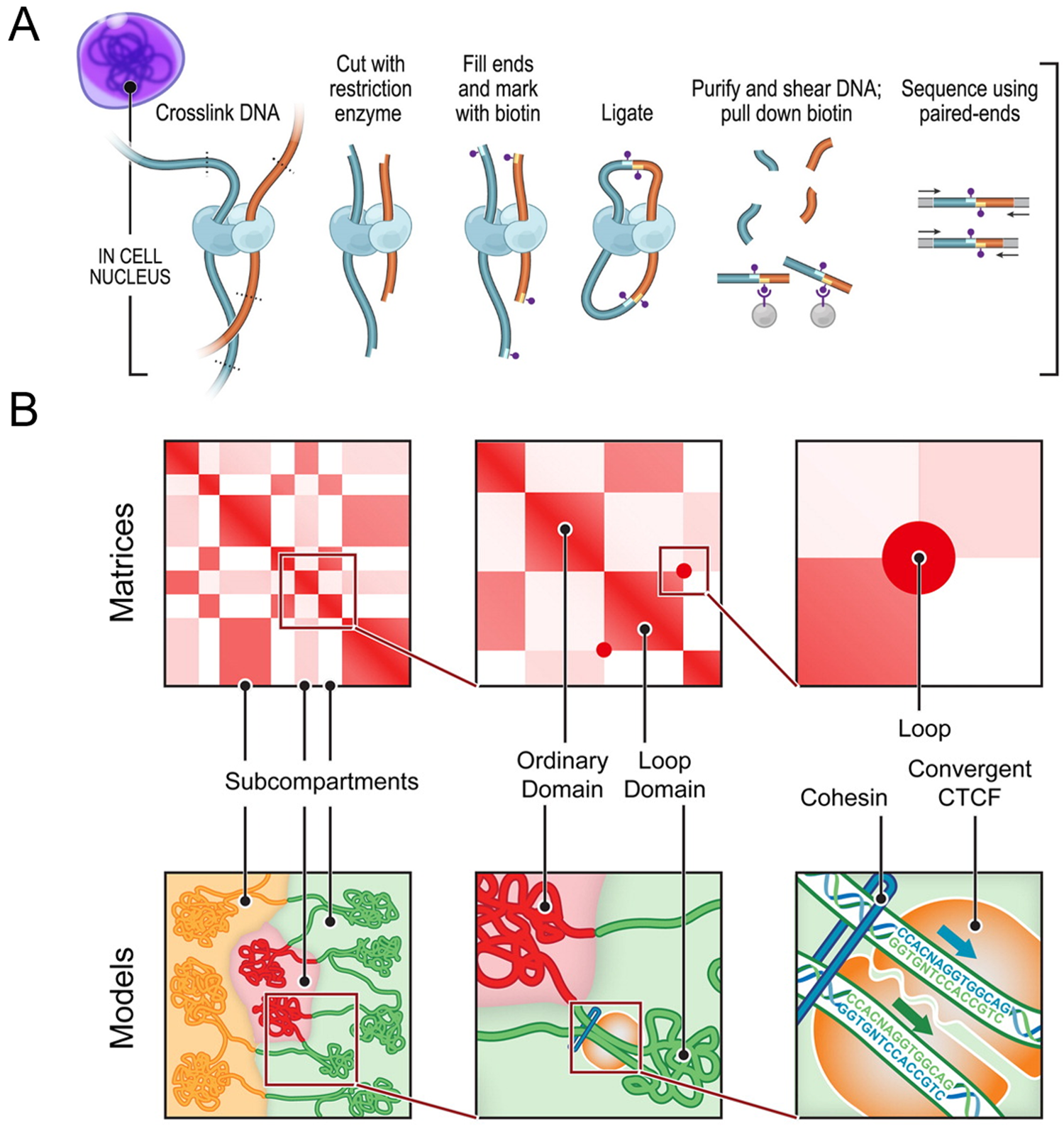
Figure 1: Chromosome conformation capture technology. (A) DNA-DNA proximity ligation assay of intact nuclei used during in situ Hi-C analysis. (B) Features capable of being revealed by Hi-C maps and corresponding cartoon representations, including subcompartments, domains, and loops. While Hi-C mapping can identify the presence of these features, exact spatial orientation is ambiguous. Figure adapted with permission from its original version [Reference Rao33].
Researchers have used 3C techniques to discover that chromosomes are packaged into territories and observe that individual chromosomes mostly interact with themselves, though they do have small regions of interaction with each other. Within a Hi-C map, it is possible to look at individual chromosomes and observe sub-features like compartments, topologically associated domains, and individual loops (Figure 1). This organization plays an important role in gene expression. For example, a loop may enable one gene to come in proximity with an enhancer that will then drive expression of that gene. On a linear scale, the enhancer is far away from the gene itself, but interaction is enabled within the loop [Reference Matthews3].
Visualizing Genomic Organization with Microscopy
Knowing the genetic composition of the genome is essential, but establishing how genes are organized with one another and their environment is equally important. Being able to visualize organization and structure on a sub-chromosomal level is necessary for understanding these relationships and how genes function. However, visualizing genomic structure at this level can prove difficult because of such a large and densely packed number of targets within the genome. There simply are not enough chromatically separable probes available to image them using conventional fluorescence microscopy methodologies. Fortunately, new approaches are beginning to allow for sequential labeling of targets using the same fluorescent probe for imaging.
Chromosome Conformation Capture Versus Imaging
Chromosome conformation capture techniques such as Hi-C are ensemble-sequencing techniques, providing an average structure of the genome from millions of cells. This provides researchers the ability to look at the entire genome at high resolution. While these techniques provide a good overview of the average cell, 3C data lose cellular context because they are based on ensemble data collection. In contrast, imaging provides data on individual cells resulting in an actual 3D representation of the conformation because distances within a genomic region are being measured directly rather than inferred, based on sequencing results. Imaging is also capable of showing relationships between multiple chromosomes within a single experiment at high resolution, which could be missed by 3C techniques. However, imaging is limited in comparison to 3C in the number of cells being analyzed, that is, tens or thousands of cells in comparison to millions. The advantage of imaging is that it provides single cell as opposed to ensemble data, enabling visualization of cellular context.
A Brief Introduction to Single-Molecule Imaging
Biological systems exist across a wide range of sizes. Light microscopy, particularly fluorescence microscopy, has been a useful tool for visualizing biological organization. However, traditional approaches are unable to resolve features below about 200 nm due to Abbe's diffraction limit [Reference Abbe4]. This is unfortunate because cells, including genomic structure, are highly organized at the nanoscale, and structure often informs function. To be able to visualize structures well below the diffraction limit using light microscopy, a variety of super-resolution techniques have been developed [Reference Hell and Wichmann5–Reference Gustafsson10]. These techniques have already made such a large impact on the field that they were the subject of the Nobel Prize in Chemistry in 2014 [Reference Betzig11–Reference Moerner13]. One such method, single-molecule localization microscopy (SMLM) [Reference Rust6], has proven to be a useful tool for imaging the genome at super resolution [Reference Nir14].
In SMLM, a diffraction-limited object is densely labeled with photoswitchable fluorescent molecules. In conventional fluorescence microscopy, the underlying structure is obscured due to Abbe's diffraction limit. With SMLM, in the presence of the correct photochemical conditions, these molecules are turned off and then turned back on in a stochastic manner. This allows the position of each molecule to be recorded during image acquisition. At the end of an acquisition, all the center points are then used to reconstruct a final super-resolution image (Figure 2). Extending this method further, it is possible to obtain 3D information by a variety of means. A common approach to 3D SMLM is the use of a cylindrical lens in the detection path, which generates an elongated point-spread function (PSF) in either X or Y, depending on the positioning of a molecule in Z [Reference Huang15]. This astigmatic approach is limited to using total internal reflection fluorescence (TIRF) or highly inclined and laminated optical sheet (HILO) illumination, and relies on point-spread-function engineering, restricting the depth of imaging from the cover slip to less than 5–10 µm.

Figure 2: Overview of SMLM. Schematic overview of single-molecule localization microscopy. Top left: Cartoon showing blurring of feature by conventional wide-field imaging. Right column: Fluorescent molecules are photochemically switched to a dark state; a sparse subset of molecules is switched back to a bright state, and their centers are localized computationally. This process of switching to a dark state, activating, and being localized is repeated many times to obtain the final super-resolution image. Bottom left: All localization molecules are compiled into one final super-resolution image with well-defined features compared to widefield.
An alternative to astigmatic imaging is biplane imaging [Reference Juette16], where a fifty-fifty beam splitter is placed in the detection path. This divides the light into two paths to be imaged on different parts of the camera. The second path is longer and uses a larger focal length lens to image onto the camera. This effectively separates the focal length of the two paths in Z (approximately 600 nm in practice), allowing two Z planes to be imaged simultaneously for the same field of view (FOV). Furthermore, prior to imaging, a calibration table is created based on the PSF of the fluorophores within each plane at known Z positions to allow the axial position of each molecule to be determined during imaging. With this approach, a single focal-plane acquisition provides axial information of 1 µm for a given focal position, and scanning the objective to image multiple focal planes allows for imaging volumes greater than 30 µm thick.
The underlying principle of SML relies on the ability to isolate a single molecule in a diffraction-limited region at a given time. There are two main methods for obtaining optical control over fluorophores that enables localization of molecules. Fluorescent proteins that switch from an “off” state to an “on” state with ultraviolet light (photo-activatable proteins [Reference Dickson17–Reference Patterson and Lippincott-Schwartz19]) or ones that shift emission spectra (photo-convertible [Reference Wiedenmann20]) can be used. A more widely used method uses organic dyes that, through a series of reversible light-driven reduction reactions, bind a side-group to the fluorophore, rendering it non-fluorescent [Reference Vaughan21–Reference Dempsey23]. The reversibility of the reaction enables a blinking behavior that allows a single fluorophore the opportunity to be localized multiple times during an experiment. While routinely used in super-resolution microscopy methods, such as (d)STORM, STORM, and GSDIM, the lack of available fluorophores with appropriate photoswitching properties makes imaging many targets in a single experiment quite challenging [Reference Dempsey24].
An alternative approach to SMLM using organic dyes without relying on photoswitching to generate blinking is a technique called Points Accumulation In Nanoscale Topography (PAINT) [Reference Sharonov and Hochstrasser25]. With this method and its derivatives, blinking is generated by the transient binding of a fluorophore to a target. When the fluorophore is bound, it appears in focus on the imaging camera, and the position can be localized. A popular use of this technique relies on DNA (DNA-PAINT [Reference Jungmann26,Reference Jungmann27]) barcoded antibodies and their complementary sequences bearing a fluorescent tag. The DNA probes are designed to be short enough so that during imaging they bind and fall off the DNA barcoded antibody, allowing only bound probes to be imaged and localized. This approach is advantageous compared to methods like (d)STORM when it comes to fluorophore selection, as fluorophores with high photon budgets (without regard for their photoswitching capabilities) can be used resulting in high localization precision. The drawback to DNA-PAINT is often the imaging time. Because it is reliant on the diffusion of probes, typical imaging times are much longer, with exposure times 5–10 times greater than (d)STORM. However, recent advancement in fluorogenic probes is making this less of an issue [Reference Chung28]. A final key advantage of DNA-PAINT is it allows for easy multiplexing [Reference Jungmann27] due to the nature of its probes (Figure 3).

Figure 3: Multiplexing with DNA-PAINT. (A) DNA-PAINT schematic. The process begins with DNA-labeled antibodies bound to the sample (A and B), shown here as primary labeled antibodies for simplicity. A solution containing oligonucleotides complementary to antibody A bearing fluorophores (A*) is applied to the sample during imaging. A* transiently binds and unbinds to A during image acquisition. A* probes are washed from the sample, so it no longer contains any fluorescent-emitting molecules. Antibody B is then labeled and imaged in the same manner using a different set of complementary oligonucleotides (B*). (B) DNA-PAINT images of microtubules (green) and clathrin (magenta), imaged sequentially.
Imaging the Genome with Single-Molecule Localization Microscopy
A natural extension of multiplexed imaging strategies like DNA-PAINT is OligoSTORM [Reference Nir14], which is the application of oligopaint probes to image the genome. This technique combines the multiplexing capabilities of PAINT with the speed of (d)STORM imaging, allowing for direct visualization of chromatin structure in situ. This technique has been used successfully to perform multi-chromosome walks. With this method, special probes made of DNA sequences that complement a genomic region are designed to label specific genes. These probes also bear a region for binding other fluorophore-labeled DNA strands that serve as imaging probes. The regions can bind longer DNA sequences for use in OligoSTORM imaging, or shorter sequences for OligoDNA-PAINT (Figure 4). The difference in the two options is that OligoSTORM relies on blinking of the fluorescent molecule to generate localizations, where the OligoDNA-PAINT localizations come from the transient binding of DNA on the sample. Having both options available also allows for the same region to be imaged twice if necessary. After developing a set of oligopaint probes, they can be imaged sequentially (Figure 4).

Figure 4: Probe design and workflow of OligoSTORM. (A) Oligopaint probe design. Probes contain a region of genomic homology and two flanking sequences, referred to as “Mainstreet” and “Backstreet,” which carry barcodes used for OligoSTORM and OligoDNA-PAINT. The design of the probes allows for each genomic region to be imaged twice if necessary. (B) Workflow of sequential rounds of hybridization. The sample begins with all oligopaint probes containing unique barcodes bound to the sample. Oligonucleotides complementary to barcode 1 and imaging strands are introduced to the sample, and barcode 1 is imaged. Oligonucleotides complementary to barcode 2, imaging strands, and toehold oligos for removing barcode 1 oligos are applied to the sample, and barcode 2 is imaged. This process is repeated, changing the toehold oligos to remove the previous round's barcode, until all barcodes have been imaged. (C) The overall workflow of an OligoSTORM experiment. It begins with the design and generation of a probe library. All probes are then hybridized to the sample in one round of hybridization. Mainstreet and Backstreet barcodes are then used to image each barcode sequentially using single-molecule localization microscopy. Data are drift corrected, and clusters are extracted using DBSCAN cluster analysis, and the final image is assembled. Figure adapted with permission from its original version [Reference Nir14].
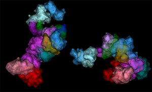
The broader workflow of these experiments involves the development of a library of many thousands of oligonucleotides and generation of OligoSTORM probes that are labeled on a sample. Fluidics are then used to label the probes individually so that each probe can be imaged by single-molecule localization. From there, data are drift corrected and analyzed so that a final image can be assembled for each genomic walk (Figure 4). This workflow has achieved localization precisions of ~20 nm in XY and 50 nm in Z, obtaining subsequent optical resolutions of ~25 nm in XY and 110 nm in Z using Bruker's Vutara SMLM platform. This methodology can provide a clear picture of analogous regions on multiple chromosomes, the relationships between sections of a single chromosome, and even finer details, such as individual loops (Figure 5). Analysis of these datasets enables generation of in situ Hi-C maps that exhibit strong correspondence to ensemble Hi-C maps, indicating the validity of image-based measurements and the overall capability of OligoSTORM to elucidate the organization of chromosomes. Furthermore, OligoSTORM data and analysis can be combined with ensemble Hi-C data to generate 3D genomic models at resolutions of 10 kb despite being imaged at much larger step sizes in a technique known as integrative modeling of genomic regions (IMGR) (Figure 5).

Figure 5: OligoSTORM imaging examples. (A) Several chromosomes traced in parallel. 8.16 Mbs of chromosome 19 was traced while also tracing chromosomes 3, 5, and 8 in uniform step sizes of 500, 250, and 100 kb, respectively. Both homologs of all chromosomes were captured. This was possible, in part, because imaging was conducted (in 100 nm increments) along the Z axis for up to 4 µm, well within the volumetric capability of the Vutara and sufficient to traverse the depth of PGP1f nuclei. (B) An isosurface rendering of maternal and paternal homologs of chromosome 19; fourteen unique barcodes are shown. (C) OligoSTORM and ensemble Hi-C data can be integrated to produce a 3D model of two homologous genomic regions in a single nucleus via integrative modeling of genomic regions (IMGR). IMGR uses rigid-body fitting and refinement through flexible fitting to achieve genomic resolutions of 10 kb or better for regions that have been imaged in much larger step sizes. Panels A and C adapted with permission from their original versions [Reference Nir14].
A Genomic Imaging Solution
Establishment of a robust acquisition and analysis pipeline complete with integrated fluidics is essential for performing large genomic walks. Bruker's Vutara SMLM imaging platform combined with integrated fluidics makes sequential imaging applications like OligoSTORM feasible for the large number of targets spatial genomics studies require. The microscope uses biplane detection making each acquisition 3D, allowing for imaging of the entire depth of the nucleus if necessary. The incorporation of the fluidics unit is critical for these types of experiments due to the large number of targets to be imaged. The fluidics unit has been carefully designed with multiplexing and single-molecule imaging in mind. Each unit has four large reservoirs for high-volume reagents, such as imaging and wash buffers, along with fifteen smaller reservoirs for more costly labeling reagents. These smaller reservoirs can be swapped out during an experiment, making imaging greater than fifteen targets possible (Figure 6).

Figure 6: Vutara ecosystem. (A) Left: Fully integrated fluidics unit that has been designed with single-molecule multiplexed and genomic imaging in mind. The unit contains four large washing reservoirs and fifteen small reservoirs for labeling reagents. The small reservoirs are swappable during an experiment, making imaging of greater than fifteen targets possible. Middle: The Vutara microscope for single-molecule super-resolution imaging. Right: An isosurface rendering of a topologically associated domain (blue) and compartment (magenta) visualized using SRX software. (B) Schematic of density-based spatial clustering of applications with noise (DBSCAN). Top left: Radius term is defined by the circles around the points. The minimum points for determining a cluster in this example is three, meaning each point must contain two additional points within its circle to be considered a core point of the cluster (blue dots). Dots reachable from a core point but not containing enough points to be a core point are also considered part of the cluster (red dots). Black dots represent points that are not reachable by any core points and are considered noise and are filtered from the final image. Top right: Cartoon representing all data points from an acquisition. Bottom right: DBSCAN is applied to the data, three clusters are identified; core points are represented by blue, grey, and dark blue dots. Red dots are reachable from a cluster and included in the final image on the bottom left.
The fluidics component is fully integrated into Vutara's SRX software at every step from acquisition to analysis. Beginning with the experimental setup, the user interface allows for full control over sequences and parameters, including flow rate, flow time, volume, and wait times. The acquisition setup also features a multi-location capture option that is useful for reducing cost and increasing throughput for experiments with long hybridization steps. After running an experiment, data can be visualized and analyzed according to probe number directly within SRX, which offers unlimited probe support.
Initial genomic imaging data can appear very noisy. SRX software offers built-in analysis tools that use the data associated with every localization to isolate signal from noise via cluster analysis. There are several algorithm options available for performing cluster analysis, including density-based spatial clustering applications with noise (DBSCAN) [Reference Ester29], ordering points to identify the clustering structure (OPTICS) [Reference Ankerst30], Delaunay analysis [Reference Alán31], and image-based clustering algorithms [Reference Bar-On32]. DBSCAN has been used to generate OligoSTORM data, and this algorithm uses particle distances and densities to assign clusters (Figure 6). Once localizations have been assigned to clusters, SRX offers a suite of statistical analysis options to calculate metrics. Some of these metrics include the number of particles in a cluster, volume, surface area, sphericity ratio, density of particles, and radius of gyration.
Bruker's Vutara SMLM imaging platform with SRX software provides a powerful system for 3D SMLM of the genome along with a wide range of other sample types. The ability to integrate fluidics with the system makes multiplexed imaging applications much more accessible, and SRX provides an all-in-one solution for data acquisition, visualization, and analysis.
Future Directions
Currently, progress is being made on integrating a workflow into SRX called ORCA (Optical Reconstruction of Chromatin Architecture) [Reference Mateo34]. ORCA uses oligopaints like OligoSTORM does but, rather than imaging at the single-molecule level, it takes sub-diffraction images at the wide-field level (Figure 7). All the fluorophores in a single genomic region are imaged as an ensemble rather than stochastically. The center of mass is determined from the image, and an ORCA walk is generated by connecting the center of masses. The technique uses small probe step sizes (2–10 kb) and is ideal for looking at smaller regions or single genes.

Figure 7: ORCA workflow and implementation in SRX. (A) An overview of ORCA workflow. A set of oligonucleotide probes is designed to label a genomic region of interest. Each segment carries a unique barcode and represents a single step of the ORCA walkthrough. Segments are imaged sequentially to build the 3D reconstruction of chromatin architecture. The 3D positioning of each segment is then used to build a distance map that is comparable to a Hi-C map. (B) A representative 3D reconstruction of chromatin architecture image visualized in SRX software. (C) A contact frequency map generated in SRX software by averaging the distance maps associated with ORCA walkthroughs of many cells. Panel A was adapted with permission from its original version [Reference Wang and Corces35].
When comparing STORM, OligoSTORM, and ORCA, decreasing the step size increases the sequence resolution. STORM gives an overview of the shape of the structure without sequence information, OligoSTORM adds in the sequence context to the structure, and ORCA results in a finer sequence resolution but does not provide the space-filling component that is obtained with OligoSTORM. The techniques are complementary, and their use depends on experimental capabilities, as well as the features being studied. ORCA is a good choice for a high-throughput study of a small genomic region, whereas OligoSTORM is preferred for taking larger steps to image a larger genomic region.
The ultimate goal is to have seamless integration within SRX of imaging data with standard genomic software platforms, and analysis for a variety of genomic imaging workflows, including ORCA and OligoSTORM. This will enable easier genomic modeling and Hi-C mapping of genomic data, helping to bridge the gap between single-cell imaging data and larger-scale data from ensemble methods.


