Introduction
Correlative microscopy refers to coordinated use of complementary techniques to study the same specimen, ideally on exactly the same area [Reference Loussert and Humbel1]. For biomedical applications correlative methods are often critical. Due to the hierarchically structured nature of bone and the inhomogeneous topographical quality of implant surfaces, multiple-length-scale 3D characterization techniques are needed to visualize bone–implant interfaces [Reference Binkley and Grandfield2]. Similarly, multiple techniques probing at different length scales are required to begin to understand the complexity of eukaryotic cells in both healthy and diseased states. Thus, correlative microscopy is an efficient way to complement and validate individual characterization techniques and to improve data analysis [Reference Wang3]. Figure 1 shows the relative capabilities, in terms of spatial resolution and elemental/chemical sensitivity of some microanalytical methods, including those employed in the work described in this article. For biomedical and health challenges, gaining a view of the full structural and chemical details at multi-length scales is essential for understanding the evolution of disease, proper diagnosis, and determining best treatment options. In this article we highlight two recent examples that used correlative microscopy methods in biomedical contexts.
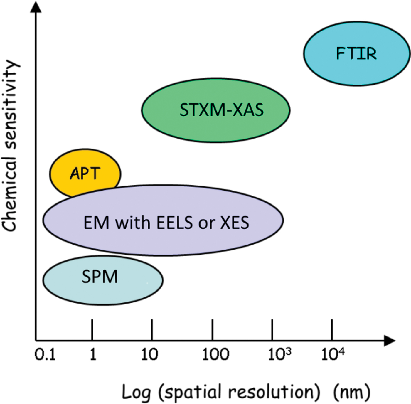
Figure 1: Spatial resolution and relative chemical sensitivity of certain microanalytical methods, including those used for correlative studies in this work. Note that techniques that are higher vertically correspond to methods that are more chemically sensitive.
Implants
Bone interfacing implants are used worldwide in the form of hip joint replacements and dental implants. Despite being generally successful, there is still an appreciable frequency of implant failures that demand revision surgeries. Degradation of the bonding between living bone and the implant device, called osseointegration, is the cause of many of these failures [Reference Grandfield4]. The physical and chemical properties of an implant surface, such as porosity, morphology, and chemical composition, are thought to play a crucial role in forming long-lasting load-bearing bonds [Reference Wang3,Reference Shah5,Reference Brånemark6]. The understanding of osseointegration has evolved as a consequence of many different microscopy and analytical studies of ever finer structures at the interface. Human bone has complex hierarchical structures with nanoscale building units of type I collagen and carbonated hydroxyapatite crystals. After a titanium implant is placed in vivo, new bone forms along the implant surface to generate a biomechanically functional integration. However, the mechanism of bone integration with nanostructured surfaces is not well understood. State-of-the-art research in this area has been generally limited to micro-scale morphological evaluations, with little compositional or nano-scale mapping at the interface. Correlative spectrometry and tomography can enable a deeper understanding of the hierarchical attachment mechanism of bone to implant.
Alzheimer's disease.
The accumulation of the peptide fragment amyloid-beta (Aβ1−42) within the brain is a characteristic hallmark of Alzheimer's disease (AD). There is evidence that metal ions, including Fe, play a crucial role [Reference Plascencia-Villa7]. The co-existence of iron and Aβ1−42 may enhance toxicity through redox-based chemistry and the generation of harmful free radicals, which can cause neuronal injury [Reference Honda8]. Thus, visualization of Fe-Aβ1−42 complexes and analysis of the Fe oxidation states therein, as well as analysis of the peptide, could provide insights into the mechanism of AD and possibly suggest approaches for treatment. Until recently, the type of iron associated with plaques was not well characterized. Using advanced electron microscopy techniques, several groups observed mineralized iron in the form of magnetite nanoparticles in Aβ plaque cores from post-mortem human cases of Alzheimer's disease [Reference Plascencia-Villa7,Reference Collingwood9,Reference Everett10]. Magnetite is not a normal feature of the human brain, so its presence suggests that aberrant iron redox chemistry might be involved [Reference Plascencia-Villa7,Reference Collingwood9]. Our work [Reference Telling11] extended this important study by using correlative electron microscopy and scanning transmission X-ray microscopy (STXM) to investigate relationships between iron biochemistry and AD pathology in the intact cortex from the brain of APP/PS1 transgenic mice, an established mouse model which over-produces Aβ peptide and reproduces the amyloid deposition characteristics of AD. We found a direct correlation of amyloid plaque morphology with iron type and levels, determined the oxidation states of nanoscale iron and their distribution in cortical tissue, supported the prior observation of magnetite involvement, and showed that Aβ-induced chemical reduction of iron in iron-amyloid complexes could occur in vivo.
Materials and Methods
Transmission electron microscopy. (TEM) is a versatile tool for probing the structure and composition of materials at near atomic resolution. In this work, TEM was used for imaging with conventional bright-field images based on mass-thickness contrast and also for high-angle annular dark-field (HAADF) imaging in scanning TEM (STEM), which provides an image intensity roughly proportional to the atomic number squared, enabling compositional contrast. Both approaches are highly useful for probing biomedical materials.
In addition to producing 2D images, TEM can be used to determine the three-dimensional morphology of objects using a technique called electron tomography (ET). By tilting a sample through a range of tilt angles and acquiring projection images at each tilt, one can use computer algorithms to reconstruct a 3D image with the resolution of the reconstruction dependent on the resolution of the individual images, the number of projections, and the range of tilt angles. In fact, HAADF-STEM tomography is an efficient technique to visualize the inhomogeneous microstructures of biomaterials and biointerfaces in three dimensions (3D) since it provides both nano-scale resolution and compositional contrast [Reference Grandfield12]. However, for a conventional thin lamellae TEM sample, the “missing wedge,” a limitation in tilt range as a result of sample thickness and shadowing at high angles, leads to two main issues: artifacts and elongation in the final reconstruction, and limited ability to combine the tilt-series with spectral information (for example, electron energy loss spectrometry, EELS). On-axis ET of a cylindrical sample removes the missing wedge and allows acquisition of high-fidelity, quantitative reconstructions of osseointegration [Reference Wang13]. Furthermore, if a cylindrical or needle-shaped sample geometry is used, on-axis ET becomes compatible with the collection of spectral information (for example, EELS or X-ray) since the specimen thickness remains constant at all tilt angles. TEM, STEM, and EELS analyses were done using an FEI Titan 80-300 TEM/STEM at McMaster University, operated at 300 keV.
Atom probe tomography (APT) is a 4D tomographic technique capable of mapping element distributions with atomic spatial resolution and parts per million chemical sensitivity. This technique is based on the evaporation of surface atoms triggered by a pulsed electric field [Reference Gault14]. With the incorporation of laser pulsing and improvements in sample preparation, APT has expanded its application base from metal and semiconductor materials to non-conductive biomaterials and minerals [Reference Langelier15,Reference Perea16]. The ions of various elements removed by laser pulsing are identified by a time-of-flight mass spectrometer via time-gated position-sensitive detectors. The resulting APT spectra (number of ions versus mass-to-charge ratios) enable the identification of chemical species. These are reconstructed into a 3D point cloud, where every point represents an elementally identified ion in the sample volume. This reconstructed volume can be further analyzed to extract and visualize the nanoscale chemical features of samples in 3D with Integrated Visualization and Analysis Software from the instrument manufacturer Cameca. However, the lack of chemical state information has always been a limitation of APT. By correlating APT with electron microscopy (i.e., ET) and spectroscopy (i.e. TEM-EELS and STXM), complementary analyses provide chemical state and crystallinity information [Reference Devaraj17]. APT was done using a Cameca LEAP 4000X HR Atom Probe at McMaster University.
Scanning transmission X-ray microscopy (STXM) is a synchrotron-based technique that routinely achieves 30 nm spatial resolution, with state-of-the art performance of 10 nm [Reference Hitchcock18]. By imaging at different photon energies, 3D (x,y,z) and 4D (x,y,z,E) data sets can be acquired, providing X-ray tomographic imaging (X-ray CT) and elemental maps through X-ray absorption spectroscopy (XAS), respectively. Details of the X-ray absorption near edge structure (XANES) spectra can provide information about the chemical state of the elements present. Multivariate statistical methods or forward fitting using reference X-ray absorption spectra on quantitative intensity scales can be used to generate quantitative maps of the chemical species present from “stacks” of full-area images at a sequence of photon energies. In this case the mapping was done by converting the measured 3D (x,y,E) data cube to optical density (OD), then fitting the OD stack to a set of reference spectra {i} extracted from distinct regions in the area measured. The (x,y,i) fitting coefficients are assembled into maps of the individual components (i), which can then be combined into a color-coded composite [Reference Hitchcock18]. In addition to identifying and mapping iron species from X-ray absorption spectra (XAS), magnetic properties can be characterized by X-ray magnetic circular dichroism (XMCD), where changes in XAS intensities are recorded with left and right circularly polarized X-rays. The XMCD signal arises from preferential excitation of electrons from core levels with orbital angular momentum >0 (e.g. Fe L23) into partly filled majority or minority spin valence energy bands. XMCD is sensitive to the direction and magnitude of the magnetic vector, and in the case of magnetite, also to the crystal site [Reference Pattrick19]. For the work described here photon energies from 280 eV to 730 eV were used. The XAS and XMCD studies were performed using the ambient STXM on beam line 10ID1 at the Canadian Light Source at the University of Saskatchewan in Saskatoon.
Results
Biomaterials Interfaces.
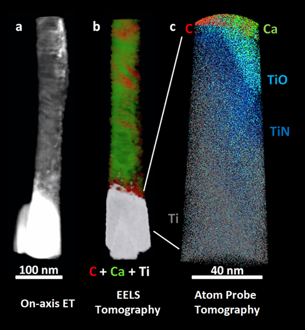
We have used chemically sensitive correlative imaging by X-ray tomography (CT), TEM, STEM, ET, APT, and STXM to investigate the 4D (3D plus composition) structure of the interface between human bone and a Ti dental implant, which had been in place for 47 months [Reference Wang3]. Figure 2 presents results from ET, EELS tomography, and APT of a FIB-machined needle-shaped sample that is about 80 nm in diameter. The Z-contrast from on-axis HAADF-STEM ET (Figure 2a) differentiates the phases in order of decreasing density: Ti implant (brightest), hydroxyapatite, and collagen/organic matter (darkest). There is evidence of continuous bone growth and integration with the surface of the laser-modified, commercially pure, titanium dental implant. This interfacial implant was shown to be rich in Ti oxide by EELS tomography, as shown in detail in reference [Reference Wang3]. Figure 2b shows the tomographic reconstruction of the series of EELS element maps on the same 80 nm needle. The reconstruction provides higher resolution elemental mapping of the interface than single raw maps from the tilt-series. Specifically, the reconstruction shows the Ca of the bone apatite (green) and the organic collagen (red). The needle was then FIB sharpened to about 40 nm diameter and analyzed by APT. The atom probe tomograph of Figure 2c shows that both Ca and C are in contact with an outer Ti oxide layer of the implant just outside a layer of TiN at the implant surface (O and N APT maps not shown). Confirmation of these phase designations was accomplished by analysis of the EELS and STXM data, as discussed below.

Figure 2: (a) On-axis ET, (b) electron energy loss tomography (EELS ET), (c) APT of the interface of human bone and a Ti dental implant. The TiO and TiN designations are related to detailed analysis of the O and N species from APT spectra [Reference Wang3]. (Adapted from [Reference Wang3]).
Correlative microscopy of a dental implant-bone interface.
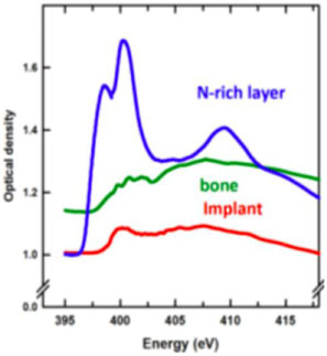
Detailed chemical speciation was provided by 2D TEM-EELS at the Ca L2,3 edge, as well as STXM studies at the C K, Ca L2,3, Ti L2,3, O K, and N K edges. Figure 3a shows a HAADF-STEM image of a bone-implant interface, and Figure 3b shows a STXM optical density difference map (OD400 eV-OD396 eV) where the N-rich region is bright and other regions show a near-background intensity. While the bone and Ti implant regions were identified from Figure 3a, the STXM OD difference image in Figure 3b clearly shows the TiN band inside the Ti implant. The color composite (Figure 3d) combines component maps generated by fitting a N 1s image sequence (50 images at photon energies between 395–420 eV) to the N 1s spectra of protein in bone (green), the Ti implant (red) and the TiN coating (blue) (Figure 3c). It is clear that the N signal in the APT data (Figure 2c) is spatially correlated with the TiN band measured by STXM. This band was probably generated from a laser hardening surface treatment of the machined implant in air [Reference Van Hove20].

Figure 3: (a) STEM image of a FIB-milled thin section of bone-dental implant interface. (b) STXM optical density difference map (OD400 –OD396. (c) N K-edge XANES spectra from regions indicated in (b). (d) STXM color-coded composite of the chemical component maps of the implant (red), bone (green), and TiNx layer (blue) derived by fitting a full N 1s stack (50 images from 395–420 eV) to the spectra in (c) (reprinted from [Reference Wang3] with permission from John Wiley & Sons). All data from STXM except (a) TEM.
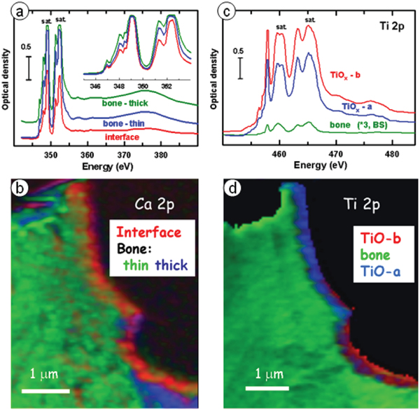
Figure 4 shows results from Ca L2,3 and Ti L2,3 STXM studies of the interface. The Ca L2,3 spectra measured by both EELS and STXM indicate the presence of multiple Ca-containing phases, with the Ca spectrum at the interface being similar to that of amorphous calcium apatite (ACP) while that of Ca in the bone was similar to that of hydroxyapatite (HA), based on detailed consideration of peak positions and shapes of the weaker Ca L-edge signals [Reference Wang3]. The Ti L2,3 signal was saturated in the region of the bulk implant, but not in the interface region or the bone. Two different Ti L2,3 signals were observed in different regions of the interface, with one having a significantly larger Ti3+ character than the other, based on the amplitude of the peak at 457.1 eV relative to the far Ti L23 continuum [Reference Wang3]. Other changes were observed in the details of the signal between 459 and 461 eV, a region well known to be sensitive to changes in the crystal structure of titanium oxides. Interestingly, a small but significant Ti L2,3 TiOx signal was observed throughout all of the bone region which was spectrally distinct from that of the titanium oxide in the interface region. This might indicate that migration of TiOx into bone can occur over long time periods. Since focused ion beam (FIB) milling can cause material redistribution, it would be useful to study a sample prepared without FIB to confirm that the Ti-in-bone was not an artifact of the FIB milling.

Figure 4: STXM speciation of bone-implant interface. (a) Ca L2,3 spectra from regions near interface. (b) Color-coded composite of component maps of three Ca-containing components derived by fitting a Ca L23 stack to the reference spectra in the insert to Fig. 4a. (c) Ti L2,3 spectra from two regions near the interface and in the bone. (d) Color-coded composite of component maps of three Ti-containing components derived by fitting a Ti L23 stack to the reference spectra in (c). Color coding in (b) and (d) matches spectral color coding in (a) and (c). (Adapted from [Reference Wang3].)
Alzheimer's Disease.
Electron microscopy and STXM were used to map protein aggregates and iron in tissue sections from APP/PS1 (Alzheimer-enhanced) mice and wild type mice. STXM was used to quantify and map iron oxidation states with nanoscale resolution. In addition, the magnetic properties of these iron deposits were studied using X-ray magnetic circular dichroism (XMCD). The latter results were found to mirror the magnetic properties of magnetite, consistent with previous work [Reference Plascencia-Villa7,Reference Collingwood9].
Correlative microscopy of amyloid structures.
We found that the cortex of APP/PS1 transgenic mice exhibited abundant iron deposits that co-localized with amyloid structures, but very few iron deposits were identified in cortical sections of wild-type mice. Figure 5 shows imaging results from the correlative TEM and STXM study of brain tissues of Alzheimer's mice [Reference Telling11]. The TEM images show the classic morphology of Aβ plaques, and the STXM Fe L2,3 map shows that Fe is co-located with these plaques (Figure 5E). Image cross-correlation analysis performed on the images shown in Figures 5D and 5E confirmed a strong correlation of pixel intensity between the images with a coefficient, R = 0.91 (20 nm pixel size), suggesting that the fibrils themselves contained iron as opposed to the presence of discrete iron foci within fibril aggregates.

Figure 5: Comparison of TEM and STXM micrographs showing a correlation of Fe with Amyloid-like fibril morphology. (A–C) TEM images from an unstained cortical section of transgenic mouse tissue measured by STXM. The high-magnification TEM image shown in (B) was obtained from the dotted area shown in (A). (D) shows TEM images of unstained fibrillar structures located in a nearby area of the same section. (E) shows a STXM-derived Fe L2,3 map (OD710–OD705) of the iron-containing fragment shown in (D). The higher-magnification TEM image shown in (F) (from dashed rectangle in (D)) is typical of Aβ plaques. (Adapted from [Reference Telling11].) All data from TEM except (E) STXM.
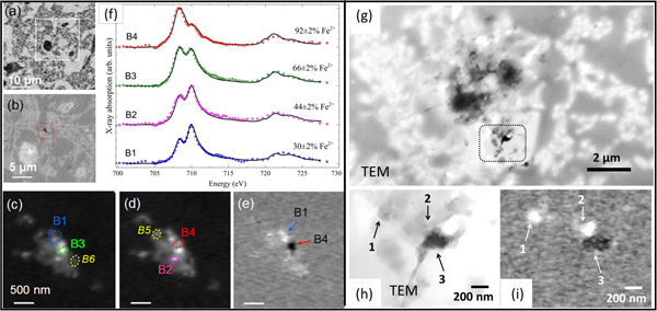
Figure 6 reveals the Fe oxidation state distributions in some Aβ plaques in more detail. Proximate but separate regions of high Fe(II) and high Fe(III) content are identified in a region of cortical thin section localized in Figure 6b (red box). Figure 6f shows Fe L2,3 XANES spectra of phases containing mostly Fe(III) to mostly Fe(II) in regions labeled B1 through B4 in Figures 6c to 6e, respectively. These results provide a profile of the oxidation states of both magnetic and non-magnetic iron phases present in each region of the iron deposit. Further XMCD analysis of these regions (not shown) revealed that the B1 region contained only a non-magnetic Fe(III) phase consistent with ferrihydrite; regions B4 and B6 contained a reduced form of magnetite together with a non-magnetic Fe(II) phase; while region B5 contained a heavily oxidized form of magnetite, which in its normal composition is a mixed Fe(II) Fe(III) species (Fe2+Fe3+2O4). The presence of different nanoscale iron oxides over a small spatial scale provides evidence for a possible redox cycling of the iron, possibly catalyzed by the Aβ deposit. Although the section shown in Figure 6(a–f) was too thick for TEM analysis, another similar area was identified that was sufficiently thin for correlative TEM and STXM (Figure 6 (g–i)). Here it can be seen that the dense particulate structure seen in the TEM image, correlates with iron in the Fe(II) oxidation state, consistent with the observation of low-oxidation state iron minerals such as magnetite and wüstite in Alzheimer's plaques.

Figure 6: STXM spectromicroscopy identification of local Fe oxidation state variations in nanoscale particulate iron in a cortical section containing Aβ plaques from a transgenic mouse sample. (a) X-ray microscopy protein map obtained by subtracting the resin background image (see supplemental to [Reference Telling11] for how the resin background was obtained) from an image obtained at the main protein absorption peak at 288.1 eV, showing the area surrounding an iron oxide deposit. Higher-magnification optical density image (b) of the boxed region in (a) showing the micrometer-sized iron deposit (dotted red box). Iron maps recorded using (c) the prominent Fe L3 peak (708 eV) and (d) the prominent Fe L2 peak (710 eV). (e) Iron oxidation distribution map [OD710–OD708], obtained by subtracting image (c) from image (d) showing localized regions of concentrated Fe(III) (bright contrast) and Fe(II) (dark contrast). (f) Corresponding Fe L2,3 X-ray absorption spectra obtained from the regions labeled B1–B4 in (c), (d), and (e). The solid lines for the spectra B1–B4 correspond to best fits to Fe(II) and Fe(III) X-ray absorption spectra. (g, h) TEM images of an unstained section of cortical tissue from the transgenic mouse tissue sample. The boxed area in (g) is shown at higher magnification in (h). (i) The corresponding iron oxidation distribution map [OD710–OD708] derived from STXM. Bright areas correspond to Fe(III) rich regions, and dark areas correspond to Fe(II) regions. The labels 1–3 indicate corresponding regions in the TEM image (h) and iron oxidation map (i). Most of the contrast in the TEM image (h) arises from density contrast by non-Fe components. (Adapted from [Reference Telling11].) All data from STXM except (g,h) TEM.
Discussion
The ability to perform measurements at several length scales with chemical sensitivity using correlative microscopy methods provides insights not available from any single method. Thus, in the bone-implant example, there are clear indications of several different Ti oxides at the bone-implant interface as well as small amounts of Ti oxide in the bone. The TiNx layer, which was observed in a very small region by APT, was unambiguously identified by STXM to be an intrinsic part of the implant surface structure. The correlative tomography workflow and associated TEM-EELS spectroscopy and STXM XANES spectromicroscopy has helped to visualize the inhomogeneous and hierarchical bone-implant interface. While the identification of Fe in the Aβ plaques could be accomplished by STEM-EELS (which was not available at the time of the study), the higher energy electron beam has been shown to cause chemical changes such as reduction of Fe(III) minerals [Reference Pan21]. The stronger spectroscopic signal and less damaging beam of STXM XANES analysis, combined with its XMCD capability, allowed measurements of the Fe chemical and magnetic state in typical TEM thin specimens.
Appropriate sample preparation is critical for these studies. It is often the case that a sample used for a lower-resolution method may need to be thinned to be suitable for a higher-resolution method. Still the correlative advantage is retained as long as the same sample region can be identified either from the intrinsic sample morphology or from fiducial markers such as letter grids. Of course the techniques used in the bone-implant study are not available to all researchers. Similarly the access to synchrotron STXM microscopes is limited. In both cases, advanced instrumentation is being acquired by many labs and more STXMs are being built (currently there are 20 operational with another 5 in development). Thus correlative approaches of the type exemplified in this article are likely to become more available in the near future. We note that this article summarizes the high points of references [Reference Wang3] and [Reference Telling11]. The interested reader should consult these references for more detail.
Conclusion
Correlative X-ray, electron, and ion microscopy approaches allow greater coverage of spatial resolution and chemical sensitivities. Such correlative microscopy often provides insights on materials structure, properties, and functions not attainable with any one technique alone. This article has highlighted two correlative studies involving STXM: an ET–APT–EELS-STXM study of a human bone-dental implant interface and a TEM–STXM study of Aβ plaques in the brain cortex of an APP/PS1 trans-genetic mouse. Together these results demonstrate the power of STXM and electron microscopy as complementary tools for correlative, multi-scale biomedical studies.
Acknowledgements
Financial support was from the Natural Sciences and Engineering Research Council of Canada (NSERC) Discovery Grant program. X.W. was supported by an Ontario Trillium Scholarship. Electron microscopy and atom probe tomography were performed at the Canadian Centre for Electron Microscopy at McMaster University, a facility supported by NSERC and other governmental sources. Prof. Anders Palmquist and Dr. Furqan Ali Shah at the University of Gothenburg are gratefully acknowledged for their significant role in the implant study cited in reference [Reference Wang3]. Scanning transmission X-ray microscopy data were acquired with the ambient STXM at the Canadian Light Source, which is supported by Canada Foundation for Innovation, NSERC, the University of Saskatchewan, the Government of Saskatchewan, Western Economic Diversification Canada, the National Research Council Canada, and the Canadian Institutes of Health Research.