


Introduction
The characterization of the three-dimensional configurations of dislocations is important to understand their influence on many important materials processes. Examples include the interaction and slip processes between individual dislocations and how these impact development of deformation microstructures, the interactions between dislocations and interfaces, and defect mitigation in epitaxial thin film growth. Moreover, the development of mesoscale dislocation simulation approaches, such as discrete dislocation dynamics (DDD), is driving a need for experimental approaches to validate these techniques (Bertin et al., Reference Bertin, Sills and Cai2020).
Although complex arrangements of dislocations are well-resolved by diffraction contrast techniques in transmission electron microscopy (TEM), particularly under weak-beam imaging conditions (Cockayne et al., Reference Cockayne, Ray and Whelan1969), information regarding feature height position is mostly lost in any single image since TEM is a projection technique. This challenge has motivated much interest in developing diffraction-contrast tomographic techniques suitable for dislocation imaging, as has been the subject of several recent reviews (Liu et al., Reference Liu, House, Kacher, Tanaka, Higashida and Robertson2014; Feng et al., Reference Feng, Fu, Lin, Wu, Huang, Zhang and Huang2020; Hata et al., Reference Hata, Furukawa, Gondo, Hirakami, Horii, Ikeda, Kawamoto, Kimura, Matsumura, Mistuhara, Miyazaki, Miyazaki, Murayama, Nakashima, Saito, Sakamoto and Yamazaki2020a, Reference Hata, Honda, Saito, Mitsuhara, Petersen and Murayama2020b).
One widely employed approach, which was pioneered by Barnard and co-workers (Barnard et al., Reference Barnard, Sharp, Tong and Midgley2006a, Reference Barnard, Sharp, Tong and Midgley2006b), is to apply intensity-based reconstruction algorithms, such as weighted back projection (WBP) or the sequential iterated reconstruction technique (SIRT), to diffraction contrast images collected over a wide tilt range but with finely spaced tilt increments. Since strain contrast is extremely sensitive to the diffracting conditions, images are usually obtained by tilting along a specific Kikuchi line, maintaining the diffracting vectors within the systemic row at fixed deviation parameters (Barnard et al., Reference Barnard, Sharp, Tong and Midgley2006a, Reference Barnard, Sharp, Tong and Midgley2006b; Liu et al., Reference Liu, House, Kacher, Tanaka, Higashida and Robertson2014), although this constraint has been relaxed in some analyses (Kacher & Robertson, Reference Kacher and Robertson2012). Intensity-based tomographic reconstruction approaches have been applied to a number of analyses of dislocations including dislocation networks in epitaxial films (Barnard et al., Reference Barnard, Sharp, Tong and Midgley2006a, Reference Barnard, Sharp, Tong and Midgley2006b, Reference Barnard, Eggeman, Sharp, White and Midgley2010), dislocations near indentation crack-tips (Sharp et al., Reference Sharp, Barnard, Kaneko, Higashida and Midgley2008; Tanaka et al., Reference Tanaka, Higashida, Kaneko, Hata and Mitsuhara2008), grain-boundary/dislocation interactions in metals (Kacher et al., Reference Kacher, Liu and Robertson2011; Kacher & Robertson, Reference Kacher and Robertson2012, Reference Kacher and Robertson2014; Chen & Yu, Reference Chen and Yu2019), and dislocation configurations in geological materials (Mussi et al., Reference Mussi, Cordier, Demouchy and Vanmansart2014, Reference Mussi, Cordier, Demouchy and Hue2017).
Although they have been applied to a number of cases, use of intensity-based reconstruction techniques for dislocation tomography does pose some challenges. First, since dynamical diffraction contrast associated with dislocations and other specimen features (such as thickness contours) does not satisfy the tomographic “projection requirement” [i.e., that the intensity vary monotonically with the projected property of interest (Midgley & Dunin-Borkowski, Reference Midgley and Dunin-Borkowski2009)], intensity-based reconstructions of diffraction-contrast images can suffer from imaging artifacts. Additionally, since many images are required to minimize errors in the intensity-based reconstructions, the acquisition of data can be tedious [e.g., requiring on the order of 50–100 images (Liu et al., Reference Liu, House, Kacher, Tanaka, Higashida and Robertson2014)], particularly given the constraint of maintaining constant diffracting conditions throughout the entire tilt series. More recently, it has been shown that intensity-based reconstructions can be performed using fewer images (e.g., 4 to 10) if the images are binarized into black and white pixels prior to tomographic reconstruction (Mussi et al., Reference Mussi, Carrez, Gouriet, Hue and Cordier2021a, Reference Mussi, Gallet, Castelnau and Cordier2021b).
An alternative approach, which we consider in this paper, is to draw on the prior knowledge that the observed curvilinear features are line objects, namely dislocations. With this knowledge, the problem can be simplified to measuring the projected two-dimensional dislocation line positions on the individual frames of the tilt series and then solving for the three-dimensional configurations of the dislocations based on the tilt geometry. Such an approach is similar in spirit to other object-based tomographic approaches, such as recent work reconstructing 3D distribution of precipitates and cavities through a simplified spherical representation (Field et al., Reference Field, Eftink, Parish and Maloy2020). A key advantage of such an object-based tomographic approach is that fewer images are required compared to intensity-based tomographic methods. Indeed, as has been demonstrated by application of the “stereo-pair” method to dislocation analyses (Basinski, Reference Basinski1964; Modéer, Reference Modéer1974; McCabe et al., Reference McCabe, Misra, Mitchell and Alexander2003; Eftink et al., Reference Eftink, Gray and Maloy2017; Jácome et al., Reference Jácome, Pöthkow, Paetsch and Hege2018; Oveisi et al., Reference Oveisi, Letouzey, Zanet, Lucas, Cantoni, Fua and Hébert2018), height information can be determined by measuring the image parallax from as few as two images collected at different tilts. In principle, however, one would expect improved precision and greater robustness to imaging ambiguities, such as those resulting from dislocation overlap, from analyses with datasets sampling more than two orientations.
In this article, we present a semi-automated approach for object-based tomography of dislocation structures and demonstrate this approach for dislocations observed in a deformed specimen of stainless steel. As we discuss, our approach can be broken into three stages: the initial extraction of dislocation line objects from the individual frames, the alignment and matching of these objects across the frames in the tilt series, and finally, the tomographic reconstruction to determine the full three-dimensional configuration of the dislocations. We demonstrate the method for a dataset collected from a dislocation network imaged by diffraction contrast scanning transmission electron microscopy (DC-STEM). Drawing on our theoretical basis for these reconstructions, we investigate the relative influence of different sources of uncertainty on the positional determinations.
Materials and Methods
Tomography Algorithm
Our object-based tomography approach is enabled by two innovations in data representation drawing on graph theory: (1) we employ a dislocation line segment-node representation for the dislocation network, using a data structure commonly employed in DDD simulations to represent our segmented image data, and (2) we employ an arc-length mapping scheme to relate the discretized lines to one another across the images.
Our tomography algorithm is broken down into three independent steps, as illustrated in Figure 1. First, the dislocation lines are extracted from each image of the tilt series and converted into a discrete representation composed of a set of straight line segments connected at nodes. For subsequent analysis, only this discrete representation is employed (i.e., we do not analyze the TEM images any further), and it is for this reason that we refer to our algorithm as being “object-based.” This contrasts with the intensity-based tomography approaches discussed above, which use a pixelized representation of the observed image intensities to perform the reconstruction. Next, the images and dislocation networks are aligned and matched with each other so that the origin and coordinate axes are consistent from image-to-image, and so that we are able to identify the same dislocation line across each of the images. Lastly, we perform the tomographic reconstruction to estimate the z-position at each point along the dislocation lines. We now discuss in detail each step of the semi-automated approach.

Fig. 1. Schematic representation of our tomography algorithm.
Our approach is implemented in MATLAB as the ObDiTo code (Object-based Dislocation Tomography). This code is available for use via the author's website (Reference SillsSills).
Line Extraction
During the line extraction step, the pixelized dislocation images are converted to a discrete set of line segments and nodes. The example in Figure 2 illustrates the approach for dislocations in 304L austenitic stainless steel observed using DC-STEM, as discussed in more detail below, but the approach can equally be applied to images collected using conventional or weak-beam dark-field transmission electron microscopy. There are two major phases to this line extraction step. In the first phase, we segment the image to identify a set of pixels associated with the observed dislocations. In our implementation, we accomplish this segmentation by first thresholding the image and then applying a “thinning” procedure, employing standard image processing procedures. We make use of several functions, denoted below by italics, that are available through the Image Processing Toolbox in MATLAB (R2020b). Unless otherwise stated, we use default parameters and settings for these functions. Other segmentation approaches optimized for curvilinear features, such as curvature-based ridge finding (Steger, Reference Steger1998) or convolutional neural networks trained on dislocation objects (Roberts et al., Reference Roberts, Haile, Sainju, Edwards and Hut2019; Holm et al., Reference Holm, Cohn, Gao, Kitahara, Matson, Lei and Yarasi2020), could also be employed. In the second phase of the line extraction, the skeletonized pixel representation is converted to an object structure defined by nodes and line segments. In the procedures below, the only place where manual input is necessary is when the skeleton is manually edited to correct errors in the pixel-based segmentation (Phase 1, Step 6).

Fig. 2. Dislocation line extraction algorithm. (a) Raw DC-STEM image of dislocations. (b) Step 2: Thresholded after denoising. (c) Step 4: De-fuzzed and cleaned up thresholded image. (d) Step 5: Line skeleton obtained by thinning the thresholded image. (e) Step 6: Skeleton after manually adding/removing lines. (f) Step 8: Final line objects with nodes and segments.
The detailed steps for these initial two phases, as depicted in Figure 2, are as follows:
Phase 1: Pixel-based segmentation
1. The image is de-noised by applying nonlocal means filtering via the imnlmfilt function.
2. The image is thresholded so that only pixels associated with dislocation lines remain. We use the local adaptive thresholding approach of Bradley and Roth (Bradley & Roth, Reference Bradley and Roth2007) via the adaptthresh function. The approach is quite simple: given a local neighborhood size around each pixel, a mean intensity within that neighborhood is computed and the pixel is thresholded as a foreground pixel if it is above some fraction α of this mean intensity.
3. The thresholded image is “de-fuzzed” by repeatedly applying a majority filter using the bwmorph function. This smooths out the edges of the thresholded regions. The filter is applied repeatedly until no pixels are changed.
4. The thresholded image is further “cleaned up” by removing “blobs” which are clearly not associated with dislocations, that is, are not long and thin. Specifically, our procedure removes a blob if its area is below a user-specified minimum value (using the bwareafilt function) or if the blob fills more than half of its bounding box (using the bwpropfilt function with the “extent” attribute).
5. The thresholded image is converted to a “skeleton” structure comprising a single row of pixels centered on each dislocation line. This is accomplished with a “thinning” algorithm (Lam et al., Reference Lam, Lee and Suen1992) via the bwmorph function (with the “thin” option). The thinning process may result in some minor imperfections in the skeleton, that is, pixel-sized holes. To remove these imperfections, we dilate the skeleton by buffering all foreground pixels with one pixel on all sides, and then thinning once more. This process produces the final skeleton.
6. The skeleton is manually edited to fix any incorrect features, such as missing lines and incorrectly identified lines. This is accomplished with a custom graphical editing tool we wrote in MATLAB.
At this point, we have a pixelized representation of the dislocation network, where each dislocation line is composed of a skeleton with the width of a single pixel. In the next phase, we convert from a pixel representation to an object representation composed of line segments connected at nodes. An important feature of the object representation is the distinction between physical nodes and non-physical nodes. Physical nodes are nodes that terminate dislocation lines where they meet a free surface and nodes where multiple dislocation lines meet, as shown in Figure 3. These nodes are physically meaningful in terms of the topology and spatial arrangement of the dislocation network. On the other hand, non-physical nodes, which are simply the discrete points along the dislocation line-object, are not topologically significant (adding and removing them does not change the network topology) and are arbitrarily located along the line. In our approach, we leverage the significance of physical nodes for object matching and image alignment.

Fig. 3. Schematic showing the basic features of our object-based tomography approach. “Top view” is the view as seen in the TEM. The dislocation network is decomposed into dislocation objects that terminate at physical nodes, with different objects denoted by different colors. In some cases, “fake” physical nodes may appear where lines cross in the TEM image.
Phase 2: Conversion to object representation.
1. The pixelized skeleton is converted to a line segment representation. First, we identify the “branch points” in the skeleton where more than one dislocation intersects via the bwmorph function. We then loop over branch points and hop from one pixel to another pixel until we encounter another branch point. During hopping, if we encounter more than l seg pixels, a node and dislocation segment is inserted.
2. The line segment representation is cleaned up by removing all dislocation objects below a minimum length L min. Here, we define a “dislocation object” as a section of line connecting two physical nodes. If one of the physical nodes on a line with length L < L min only has one connection (i.e., it intersects a free surface), then we simply delete that line. If both physical nodes have more than one connection and L < L min, then to delete the line we must merge the nodes together (i.e., we cannot simply delete the line) in order to conserve the network topology.
At the end of this process, the image has been converted to a structure characterized by a set of nodes with coordinates r and an array of segments S containing pairs of nodes. Line extraction must be performed on each image to be used for the tomographic reconstruction.
Object Matching
Before we can perform a reconstruction using the dislocation network line objects obtained using the procedure in the section “Line extraction,” we must match the dislocation objects identified in the individual frames to their corresponding objects across the full data series, a process we call object matching. In other words, we must identify the same dislocation object across each image. This procedure is not trivial to accomplish for several reasons. First, as the sample is tilted, the dislocation lines move, making their position from image-to-image slightly different. Second, as the sample is tilted, lines that are separate from each other in one image may overlap in another image. This introduces spurious physical nodes where it appears that two dislocations intersect each other, but in reality they do not (see Figure 3); we call these features “fake” physical nodes. Fake physical nodes change the apparent topology of the dislocation network, making it difficult to relate networks from different images to each other.
While, in principle, it should be possible to develop an automated procedure for object matching, given the above complications it is difficult. We chose instead to develop a graphical tool to allow a user to manually match physical nodes across images. To this end, we require that each dislocation line is uniquely identified by the pair of physical nodes that bound it. In other words, we require that two physical nodes that bound a dislocation object are never connected by more than one dislocation line. This approach is akin to viewing the dislocation network as a simple graph (no multiple edges, i.e., edges that connect the same nodes), comprising a set of edges connected at nodes. Each dislocation object is an edge of the graph, and its bounding physical nodes are the graph nodes. The requirement that there are no multiple edges in the graph seems restrictive, but since there is a high degree of flexibility in how each dislocation object is defined it should not be difficult to satisfy this requirement in practice. See Figure 3 for an example of how a network can be decomposed into dislocation objects. Using the manual object matching tool, physical node pairs are matched up across the images. The dislocation objects (edges) connecting those physical nodes are then extracted from the overall network. The user may match as many or as few physical node pairs as desired (i.e., the whole network does not have to be matched). Also, an edge does not have to be identified in every image from a tilt series (e.g., reconstruction is possible using as few as two images worth of information for a dislocation object).
Tomographic Reconstruction
In our tomographic reconstruction, we define an imaging coordinate system with the tilt axis in the y-direction, the z-direction opposite the electron beam direction, and the x-direction implied by the right-hand rule. The imaging plane is the x–y plane, so rotation about the tilt axis induces motion in the x-direction in the imaging coordinate system (see Appendix A). Determination of the z-height out of the imaging plane of each point on the dislocation lines is the fundamental goal. We assign one image as our reference image, which is used to define the configuration in which we will perform the reconstruction. For example, the coordinate of node i in the reference image with tilt angle ω ref is  $( x_i^{{\rm ref}} , \;y_i^{{\rm ref}} , \;z_i^{{\rm ref}} ) , \;$ and we seek to determine $z_i^{{\rm ref}}$. On the other hand, for image j the tilt angle is ω j ≠ ω ref, so the x-coordinate of node i in image j is $x_i^j \,\ne \,x_i^{{\rm ref}}$. Our basic approach for tomographic reconstruction leverages the relationship between z-position and x-position in the imaging coordinate system as the specimen is tilted. Specifically, basic geometry reveals (see Appendix A) for the same point on a dislocation line the z and x-coordinates are related as
 $$f_i^j = z_i^{{\rm ref}} {\rm sin( }\omega ^j-\omega ^{{\rm ref}}), $$
where  $f_i^j \equiv x_i^j -{\rm cos( }\omega ^j-\omega ^{{\rm ref}}) x_i^{{\rm ref}}$. Hence, the change in x-position as the tilt angle is varied is linearly related to the z-position in the reference image. If we extract the set of x-coordinates from all images, we can determine the z-coordinate $z_i^{{\rm ref}}$ through a linear regression of $f_i^j$ versus sin(ω j − ω ref).
Before we can proceed with obtaining  $z_i^{{\rm ref}}$ however, three challenges remain: (1) the images must be aligned so that their tilt axes are coincident, (2) we must orient the images so that the tilt axis is along the y-axis (since the tilt axis may be arbitrarily oriented in the x–y plane), and (3) we must determine how to find “equivalent” points on the same dislocation line from image-to-image. Challenge 1 is easily solved by noting that the centroid of the dislocation structure does not move as the sample is tilted. We can estimate the centroid of each image by computing the mean position among the set of physical nodes which have been matched across all images (recall that physical nodes do not have to be matched in all images). Let the set of physical nodes which have been matched across all images be ${\cal M}$. The resulting mean position for image j is then
 $$( \bar{x}^{\,j}, \;\bar{y}^{\,j}, \;\bar{z}^{\,j}) = \displaystyle{1 \over {N_{\cal M}}}\mathop \sum \limits_{i\in {\cal M}} ( x_i^{\,j} , \;y_i^{\,j} , \;z_i^{\,j} ), $$
where  $N_{\cal M}$ is the number of nodes in ${\cal M}$. We then align the images by subtracting the mean position of each image from all nodal coordinates within that image. To solve challenge 2, we must determine the orientation of the tilt axis relative to the vertical (y) axis of the images (we assume that the tilt axis is always in the plane of the image and that its orientation is the same in every image). The tilt axis will form an angle α with the vertical axis of the images. We estimate α by performing a linear regression of $x_i^{\,j}$ versus $y_i^{\,j}$ for the matched nodes in ${\cal M}$, the slope of which is related to α via the inverse tangent operator.
Resolving challenge 3 is the most difficult aspect of object-based tomography. The basic issue is that, in general, the nonphysical nodes obtained in each image are not directly related to each other, because they are the result of an arbitrary extraction process. For example, it is highly unlikely that nodes will be placed at the exact same spot on a given dislocation line across all images. But in order to utilize equation (1), we must collect the x-coordinate from each image at the exact same spot. To accomplish this, we need a mapping that relates all points on each dislocation line from one image to another. We establish such a mapping using the graph description of the dislocation network; within the graph for each image, we know that two dislocation objects correspond to the same dislocation if they share physical nodes. This reduces our mapping problem to relating the points within a given pair of objects (from different images) with the same (matched) physical nodes. To accomplish mapping within a single object, we introduce the notion of a relative y-arc length mapping. We define the y-arc length as the total absolute change in y-position over some trajectory through the x–y plane. We can state this mathematically by defining the y-position of the dislocation object parametrically as y(t), where t varies from 0 to 1 from the beginning to the end of the dislocation object. Accordingly, the y-arc length from t = 0 up to some position t′ on the object is
 $${\Upsilon ( }{t}^{\prime}) = \int_0^{{t}^{\prime}} {\left\vert {\displaystyle{{dy( t) } \over {dt}}} \right\vert } dt.$$
The relative y-arc length is then defined as
 $${\bar{\Upsilon }( }{t}^{\prime}) \,\equiv \,\displaystyle{{{\rm \Upsilon ( }{t}^{\prime}) } \over {{\rm \Upsilon ( }1) }},$$
that is, the y-arc length at t′ divided by the total y-arc length for the edge. In practice, we compute the y-arc length using the discrete segments in our networks by summing the absolute value of the difference in y-coordinates between the nodes bounding each segment (or interpolating between the nodes to obtain the y-arc length in the middle of a segment). In our mapping framework, we assume that two points of equivalent relative y-arc length on the same object are identical points in space. Because of the fact that all lengths in the y-dimension (parallel to the tilt axis) are conserved as the specimen is tilted, this mapping is exact as long as the dislocation line extraction is exact. Obviously, line extraction is inexact, so there is error in the y-arc length mapping. In Section “Uncertainty analysis,” we perform an uncertainty analysis to explore how sensitive the accuracy of the reconstruction is to error in the line extraction.
To summarize the above discussion, the steps of the tomographic reconstruction are as follows:
1. Shift all datasets so that their tilt axes are coincident. This is accomplished by computing for each image the mean position of all physical nodes which have been matched across all images, and then subtracting the respective mean position from each image.
2. Rotate datasets so that the tilt axis is coincident with the vertical (y) axis. The orientation of the tilt axis is determined through a linear regression of the (x,y) coordinates of the physical nodes which have been matched across all images.
3. Compute the relative y-arc length of each dislocation object in the aligned dislocation networks. This is done by summing the difference in y-coordinates of all segments in each edge.
4. For each node i in the reference image, determine $x_i^{\,j}$ for each image j using the relative y-arc length mapping. This means we determine $\bar{{\rm \Upsilon }}_i^{{\rm ref}}$, the relative y-arc length for node i in the reference image, and then determine $x_i^j = x( \bar{{\rm \Upsilon }}_i^{{\rm ref}} )$, where $x( \bar{{\rm \Upsilon }})$ is the x-position of the same edge in image j at relative y-arc length $\bar{{\rm \Upsilon }}$ obtained by interpolating the nodal data.
5. Determine the z-position of each node using equation (1).


This concludes the reconstruction algorithm. We emphasize that the essential ingredients of the reconstruction algorithm are: (1) the graph representation of the dislocation networks which enables us to relate the images together on the basis of physical nodes by matching edges of the graph (dislocation objects) up with each other and (2) the relative y-arc length mapping which allows us to unambiguously map between any point on a pair of matched objects.
Electron Microscopy
To illustrate the application of our approaches, we analyzed dislocations observed in a specimen of forged austenitic stainless steel (304L). Details regarding this material and its overall microstructure have been discussed previously (Sabisch et al., Reference Sabisch, Sugar, Ronevich, Marchi and Medlin2021). The TEM specimen for this work was prepared by electropolishing. After initial mechanical thinning to a thickness of 150 μm, the specimen was jet polished (Struers, Tenupol-5) in a solution of 10% perchloric acid and 90% ethanol at a temperature of −12°C, potential of 24.1 V, and current of 61 mA. The specimen was observed using an FEI Titan TEM, operated at 200 keV. Images were collected using the diffraction-contrast STEM approach (Phillips et al., Reference Phillips, Brandes, Mills and De Graef2011), with a convergence angle of 4.03 mrad and collecting the selected diffracted intensity using an annular dark-field (ADF) detector. We maintained a weak-beam diffracting condition (approximately 2.5 g) using a {111} systematic row. We employed an objective aperture to limit the signal reaching the ADF detector to that from the 2 g reflection. We have found that this condition gives a good balance of image contrast and image localization. The tomographic tilt series was conducted using a conventional two-axis double-tilt holder. We tilted about the {111} systematic row over a range of angles, making fine adjustments to the tilt to ensure that the diffracting conditions remained constant through the series. The maximum positive and negative tilt were limited by interference with the microscope's objective aperture.
Results
Reconstruction Algorithm Verification
To verify the details of our reconstruction algorithm—specifically the graph-based alignment and y-arc length mapping—we constructed synthetic TEM datasets by producing three-dimensional dislocation networks composed of straight line segments, and then “imaging” these networks via two-dimensional projections after tilting to various angles. This approach allows us to validate that our algorithm and code are correct since we know the exact z-coordinates of the synthetic datasets. It also allows us to assess sensitivity to various sources of uncertainty in the imaging and extraction processes. By analyzing synthetic datasets of varying degrees of complexity, including a snapshot obtained from a DDD simulation as shown in Figure 4, we have verified that our tomography algorithm is “perfect” in the sense that the exact solution is recovered in the absence of noise in the positional data. This result verifies that our algorithm is sound and that the y-arc length mapping is an appropriate approach for relating images to each other.

Fig. 4. Synthetic dataset from discrete dislocation dynamics simulation used for algorithm verification. (a) Top and (b) isometric views.
Uncertainty Analysis
Using our synthetic data, we can analyze the uncertainty of the reconstruction in the form of the amount of error in the reconstructed z-position relative to the actual z-position. We consider the error in reconstructing straight dislocation lines of length L. Each line is oriented so that its angle from the tilt axis in the plane x–y is θ and its angle out of the x–y plane is ϕ (see Fig. 5). Using this approach, we can assess how the uncertainty varies as the line orientation (θ, ϕ) varies. In each synthetic dataset, we insert 20 dislocation lines and introduce various types of noise into the projected images used for reconstruction, as discussed below. Lines were inserted into an area of approximately 2 L by 2 L. We repeat this process 1,000 times to fully populate an average error surface in (θ, ϕ) space.

Fig. 5. Line geometry used for error analysis.
Below we consider three different types of error: uncorrelated positional error, correlated shift error, and correlated rotational error. Uncorrelated positional error is modeled by randomly shifting each node within its respective image plane according to a zero-mean normal distribution with standard deviation δ us. This error simulates uncorrelated noise in the dislocation lines and errors in the line extraction procedures which may induce unphysical “fluctuations” in the line profile. Correlated shift error is modeled by randomly shifting each node on a dislocation object within the x–y plane by the same amount prior to tilting and producing a synthetic image. The shift vector for each line is obtained by sampling a zero-mean normal distribution with standard deviation δ cs. This error simulates shifting that may occur if the apparent positions of the dislocation objects shift relative to each other during tilting as a result of contrast variations. Finally, correlated rotational noise is modeled by randomly rotating each object within the image plane for each image. The amount of rotation is obtained by sampling a zero-mean normal distribution with standard deviation δ cr. Such errors could arise, for instance, in tomographic acquisitions obtained using a tilt-rotate holder rather than a conventional two-axis double-tilt holder.
To quantify the error induced by each type of noise, we computed the average error in z-height Ez of each dislocation line. We then binned up (θ, ϕ) space into bins of width 4.5° and averaged over the error of all replica lines within each bin. The resulting error surfaces are presented in Figure 6 with noise parameters of δ us/L = 0.01,  $\delta _{\rm cr} = 2^\circ , \;$ and δ cs/L = 0.01. Synthetic TEM images were spaced apart by 3° tilt increments using tilt ranges of ±3° (3 total images) and ±12° (9 total images). A segment length of l seg/L = 0.1 was used. The following conclusions can be drawn. First, the error magnitude drops by about an order of magnitude upon increasing the tilt range from ±3° to ±12°, demonstrating the importance of a wide tilt range. Second, the trends in (θ, ϕ) space are different for each type of error. Uncorrelated shift error is most significant near $\theta = 90^\circ$ and, to a lesser extent, near $\phi = 90^\circ$. In contrast, correlated rotation error is most significant when $\theta < 60^\circ$ and $\phi < 60^\circ$. Finally, correlated shift error does not exhibit any sensitivity to θ and ϕ. In terms of error magnitude, for the chosen error parameter values the reconstruction error is in the range of 0.01 L to 0.05 L when $\theta < 70^\circ$ and $\phi < 80^\circ$. When $\theta > 70^\circ$, the error due to uncorrelated shift noise increases precipitously, likely rendering an accurate reconstruction impossible for lines in this angle range. This is because it becomes incredibly difficult to clearly distinguish points on the dislocation line from each other, which manifests by the relative y-arc length mapping breaking down. We note that this problem is not unique to our algorithm; any dislocation tomographic reconstruction algorithm will suffer large errors when θ is close to 90°.

Fig. 6. Results from uncertainty analysis showing average error in z position divided by the line length, Ez/L, for different types of error with tilt series at 3° increments over tilt range [ − |ω|, + |ω|]. First column: uncorrelated shift noise with δ us/L = 0.01; second column: rotational error noise with  $\delta _{\rm cr} = 2^\circ$; third column: correlated shift noise with δ cs/L = 0.01. Top row: tilt range $\vert \omega \vert = 3^\circ$; bottom row: tilt range $\vert \omega \vert = 12^\circ$. Each image series had 20 randomly oriented lines with segment length l seg/L = 0.1.
Figure 7 shows how the number of images taken over a ±12° tilt series influences the average error when all sources of noise are applied simultaneously using the same noise parameters as above. First, we note by comparing the “9 images” result with the bottom row of Figure 6, obtained using the same conditions, that the different error modes seem to combine in an additive manner; the error surface obtained in Figure 7 is close to the sum of all errors in the bottom row of Figure 6. Second, Figure 7 shows that the error reduces at a slow rate as the number of images is increased. For example, increasing the number of images by six results in about a 1% reduction in average error. The region of large error near  $\theta = 90^\circ$ also shrinks as the number of images is increased.

Fig. 7. Error due to combined noise showing the influence of the number of images over a ±12° tilt series. Noise parameter values: δ us/L = 0.01,  $\delta _{\rm cr} = 2^\circ$, δ cs/L = 0.01.
Finally, in Figure 8, we show how the reconstruction error increases as the uncorrelated shift error increases, with values of δ us/L = 0.025, 0.5, and 0.1. Figure 8 shows that the average reconstruction error increases sublinearly as δ us/L is increased (i.e., doubling δ us/L does not double the reconstruction error). When δ us/L is largest, the reconstruction error is relatively insensitive to the line orientation angles (a flat error distribution), but is still largest near  $\theta = 90^\circ$. Based on these results and expected positioning errors in dislocation line extraction, we estimate the average reconstruction error to be about E z/L ≈ 0.1.

Fig. 8. Error due to combined noise showing the influence of magnitude of uncorrelated shift error, δ us/L, with a ±12° tilt series and 9 images. Other noise parameter values:  $\delta _{\rm cr} = 2^\circ$, δ cs/L = 0.01.
Dislocation Network in Forged 304L Stainless Steel
To illustrate the use of our algorithm, we apply it to dislocations observed in the forged 304 L stainless steel specimen. Figure 9 shows DC-STEM images of the specimen taken over a single-tilt series at tilt angles of −11.87, −2.38, 2.38, 7.11, and 11.87 degrees (an image was also taken at −7.11 degrees, but line extraction was difficult with this image due to contrast effects resulting from the proximity of this tilt condition to the ⟨110⟩ zone axis). The dislocation network in the sample is quite complex, as shown in Figure 9a. Extended dislocations/nodes are visible in a number of places owing to the low stacking fault energy of this stainless steel alloy (Meric de Bellefon et al., Reference Meric de Bellefon, van Duysen and Sridharan2017); this further complicates the reconstruction, which assumes perfect (unextended) dislocations. For simplicity, we consider a smaller portion of the image for tomographic reconstruction, the boxed portion of the image. We also mark in Figure 9 a few reference points A, B, and C within each image to help relate images to one another; we will continue marking these points in our analysis below.

Fig. 9. DC-STEM images of a forged stainless steel sample used for tomographic reconstruction. (a) Full field of view showing boxed portion used for tomography. (b–f) Boxed portion at tilt angles (b) ω = −11.87, (c) −2.38, (d) 2.38, (e) 7.11, and (f) 11.87 degrees. The labels A, B, and C show reference points for comparison with extracted lines (in Fig. 10) and tomographic reconstruction (in Fig. 13).
After matching up the same dislocation objects across all images, we used the physical nodes that were present in all images to re-center the networks and determine the orientation of the tilt axis. Note that one dislocation in the network (the “C” shaped line in the top left) was only fully visible in three out of five images, and so its physical nodes were not used during re-centering. The re-centered dislocation networks are shown in Figure 10. The dataset used to estimate the tilt axis inclination is shown in Figure 11, with all points for each physical node shifted by the mean x and y values and collected together. Note that there is considerable scatter in the data, indicating the degree of uncertainty in the line extraction.

Fig. 10. Re-centered dislocation networks with coincident tilt axes. Large markers denote physical nodes. Labels A, B, and C refer to positions marked on the original data in Figure 9.

Fig. 11. Determination of the tilt axis inclination α. Each data point corresponds to a physical node. If the dataset was perfect, all points should fall on a straight line.
Next, we perform the tomographic reconstruction on the matched dislocation objects. Examples of fits to equation (1) for two nodes are given in Figure 12, showing a node with (a) a good fit and (b) a poor fit. The poor fit in (b) results from the dislocation line being orthogonal to the tilt axis (i.e., θ ≈ 90°), resulting in a large uncertainty as shown in the section “Uncertainty analysis”. As a result, the z height of the node cannot be determined accurately. In general, when the dislocation line is not close to being orthogonal to the tilt axis, the fit to equation (1) is reasonably good.

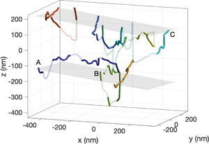
The final 3D reconstruction is presented in Figure 13 using the image with ω = 7.7° as the reference image. Each dislocation object is colored differently. Using the physical nodes connecting only one object (e.g., at a free surface), we also estimate the position and orientation of the TEM foil surfaces as gray planes obtained by linear regression. To differentiate nodes with a high degree of uncertainty, we have set some line segments to be transparent. We identify a node as being “uncertain” if any of the three following criteria are met: (1) the segments connecting the node form an inclination angle of θ > 80° relative to the tilt axis (y-axis in Fig. 13); (2) the R 2 value for the fit to equation (1) is less than 0.7 indicating a large degree of scatter in the extraction data; or (3) the y-intercept from the fit to equation (1) is greater than 40 nm (according to equation (1), the y-intercept should be zero). Criterion 1 accounts for the inherent uncertainty when θ is close to 90°. Criteria 2 and 3 account for inconsistencies in the data due to imaging or extraction uncertainties. We note that some of the lines are found to be “outside” the estimated foil thickness. This is a result of position error from the reconstruction.

Fig. 13. Tomographic reconstruction of the dislocation network. (a) Isometric and (b) “unfolded” views. Each graph edge is colored with a unique color. Line segments with large uncertainty are semi-transparent (see text). Gray planes denote estimated surfaces based on physical node positions. Labels A, B, and C refer to positions marked on the original data in Figure 9. Markers O and □ denote the nodes used for Figures 12a and 12b, respectively.
Examining the three-dimensional reconstruction, we see that the dislocation content is distributed through the thickness of the TEM foil, a fact that is not obvious from individual images. For example, based on a single image, the “box” structure in the lower right corner may be interpreted as an interconnected network feature. However, the reconstruction reveals that the far right (orange) line forming the box is in an entirely different plane. Another interesting feature is that the “hard corners” in several of the dislocation lines (e.g., the dark blue line) are not associated with significant changes in plane orientation.
Discussion
We have developed an object-based tomography algorithm with the following advantages over existing approaches: (1) Fewer images are required to attain the same level of positional accuracy (our error analysis shows good accuracy with as few as 3 images); (2) the technique is conceptually simpler than pixel-based approaches since the reconstruction derives from simple geometry; and (3) the technique is inherently consistent with the line nature of dislocations.
In its current implementation, our method is semi-automated and still requires several manual operations. Two primary challenges, which we discuss next, remain to be resolved before the approach can be fully automated.
One challenge is the automated extraction of dislocation line objects from TEM images. Often the contrast of the dislocation lines varies, resulting in “low spots” in intensity in the middle of lines. Also, it can be difficult to distinguish true dislocation lines from unphysical noise. In some cases, it is not possible to unambiguously identify dislocation lines by hand, let alone with an automated subroutine. When applied to the stainless steel dataset presented here, our extraction algorithm successfully extracts ~80% of the true dislocation line content while also extracting some unphysical “lines.” We employed a relatively simple, standard thresholding approach for segmenting the dislocations (Bradley & Roth, Reference Bradley and Roth2007). Further improvements could be made in the approach by employing segmentation algorithms specialized for curvilinear features characteristic of dislocation lines, such as curvature-based techniques (Steger, Reference Steger1998) or machine learning (Roberts et al., Reference Roberts, Haile, Sainju, Edwards and Hut2019; Holm et al., Reference Holm, Cohn, Gao, Kitahara, Matson, Lei and Yarasi2020). If the image thresholding is accurate, the final “thinning” step and conversion to segment-based representation is expected to be accurate as well. Hence, improvements to the segmentation algorithm should be a major focus going forward.
A second challenge for automation is relating the dislocation objects from one image to another. Because our approach utilizes a graph representation of the network to relate dislocation lines across images to each other, it requires that the dislocation networks from each image be topologically consistent. This means that physical nodes must be the same from image to image so that graph edges (dislocation objects) can be matched. Physical nodes associated with points at which the dislocation lines exit the foil are relatively easy to identify. On the other hand, physical nodes at the intersection of dislocation lines are more challenging to identify. This difficulty arises because the projection of two overlapping dislocation lines, which pass above or below each other but do not actually touch (e.g., the orange line in Fig. 13), will erroneously appear in any single image as a physical node. Distinguishing these “fake” physical nodes from true physical nodes is challenging. For the dataset analyzed here, such fake physical nodes were identified by hand and ignored. However, in principle, the tomographic reconstruction can help to identify fake physical nodes. Specifically, fake physical nodes are associated with multiple graph edges (dislocation objects). If they are true physical nodes, the z-height determined from each edge should be approximately the same. If instead the physical node is fake and not connected to one or more of the graph edges, the z-heights will differ significantly. Thus, it should be possible to iterate in the reconstruction, to systematically eliminate such “fake” physical nodes.
Of all the steps in our tomography approach, the object matching step is the most time-consuming because it requires manually identifying identical graph edges across images. In principle, this step could be (at least partially) automated using a graph network alignment algorithm; in graph theory, aligning (e.g., relating) graphs to each other is a common problem and many algorithms have been developed (Emmert-Streib et al., Reference Emmert-Streib, Dehmer and Shi2016; Trung et al., Reference Trung, Toan, Vinh, Dat, Thang, Hung and Sattar2020). However, graph network alignment is especially difficult when graphs are not topologically identical, such as the case here where fake physical nodes may pollute the topology of one image. Thus, the extension of graph network alignment algorithms to work robustly for complicated topologies will be critical to fully automating object-based dislocation tomography. An alternative approach is to use machine learning techniques. Altingövde et al. (Reference Altingövde, Mishchuk, Ganeeva, Oveiisii, Hebert and Fua2022) recently developed a convolutional neural network for matching dislocations in a stereo image pair. This technique could be extended to match dislocations across more than two images.
The error analysis we presented in the section “Uncertainty analysis” was focused on quantifying the error in the reconstructed z-positions for a straight dislocation line. This provides a simple case study to clearly demonstrate how the error is sensitive to the line orientation relative to the tilt axis. However, in practice, many users may be more interested in quantifying features of the dislocation network with curved lines, such as the dislocation density of each slip system, rather than the precise z-positions of lines. Quantifying our method's ability to extract such features as slip system density in an arbitrary network is more challenging and requires additional study. Based on the results in the section “Uncertainty analysis,” we can nonetheless conclude that when dislocation lines are nearly orthogonal to the tilt axis it becomes quite difficult to accurately extract any quantitative feature of the dislocation network.
Finally, we discuss the broader application of the object-based tomography technique as we have constructed it. Fundamentally, the technique presented above only works for 1D objects because it relies on the relative y-arc length mapping [equation (4)] to identify equivalent points on dislocation lines in each micrograph. This mapping only works for line objects, but these line objects could be features of multidimensional objects. For example, the method could reconstruct edges of grain boundaries, stacking faults, or stacking fault tetrahedra as long as the same edges are identified in each image. The method cannot reconstruct points away from the edges, however. Conceivably the method could be extended to reconstruct 2D surfaces by including a relative x-position mapping in addition to the y-position mapping, so that points in between the edges could be mapped as well. However, if the surface has a complex (e.g., nonsmooth) morphology this may be difficult to accomplish.
Conclusion
We have demonstrated a semi-automated, object-based method for dislocation tomography. This method draws on the prior knowledge that dislocations are line objects and as such the approach requires far fewer individual images in the tomographic tilt series than conventional intensity-based tomographic reconstruction methods. The method employs a dislocation node-line segment representation and an arc-length mapping scheme to relate the dislocation objects between individual frames. This approach can be straightforwardly applied to tilt series of dislocation images using any diffraction contrast technique. Key steps for further automating the approach include improving the line extraction processing and advancing graph network alignment algorithms to be robust to apparent topological inconsistencies resulting from the overlap of nonintersecting dislocations.
Acknowledgments
The authors thank Mark Homer for assistance with the TEM specimen preparation, Dr. Joe Ronevich for provision of the material, and Dr. Rohit Singh for discussions on graph network alignment. Sandia National Laboratories is a multimission laboratory managed and operated by the National Technology and Engineering Solutions of Sandia, LLC, a wholly owned subsidiary of Honeywell International Inc. for the U.S. Department of Energy's National Nuclear Security Administration under contract DE-NA-0003525. This paper describes objective technical results and analysis. TEM observations were conducted under the user program at the Molecular Foundry (Lawrence Berkeley National Laboratory), which is supported by the Office of Science, Office of Basic Energy Sciences, of the U.S. Department of Energy under Contract No. DE-AC02-05CH11231. Any subjective views or opinions that might be expressed in the paper do not necessarily represent the views of the U.S., Department of Energy or the United States Government.
Conflict of interest
The authors declare that they have no competing interest.
Appendix A: Geometry of tomographic reconstruction
To establish the relationship between the tilt angle ω and the z-height, consider the geometry in Figure A.1. In the reference “image,” a point on a given dislocation line has unknown z-height z ref and x-position x ref relative to the tilt axis and the plane normal to the electron beam direction (i.e., the imaging coordinate system). The line connecting this point with the tilt axis has length l and makes an angle ψ with the x-axis. This sample is then tilted by an angle ω about the tilt axis resulting in a new x-position x j in the imaging coordinate system. Our goal is to relate the change in x-position during tilting to the z-height in the reference image. Using basic trigonometry, we can establish the following relationships:
 $${\tan}\psi = \displaystyle{{z^{{\rm ref}}} \over {x^{{\rm ref}}}},$$
 $${\cos}\psi = \displaystyle{{x^{{\rm ref}}} \over l},$$
 $${\cos( }\psi + \omega ) = \displaystyle{{x^j} \over l}.$$
Fig. A.1. Geometry for performing the tomographic reconstruction.
Using the trigonometric identify cos(ψ + ω) = cosψcosω − sinψsinω in conjunction with equations (A.2) and (A.3) gives
 $${\cos}\psi {\cos}\omega -{\sin}\psi {\sin}\omega = \displaystyle{{x^j} \over {x^{{\rm ref}}}}{\cos}\psi. $$
Dividing by cosψ, using equation (A.1), and rearranging leads to our final result, equation (1).


 Open access