


Introduction
The three-dimensional (3D) morphological (e.g., size and shape) and spatial (e.g., orientation, connectivity, size or shape sorting, and porosity) characteristics of a system encode a wealth of information about internal processes and physical properties. As a result, when measured accurately, 3D attributes are important for a variety of scientific and industrial applications spanning a wide range of spatial scales. Unfortunately, the acquisition of 3D data often is nontrivial. Certain recent advancements, such as photogrammetry and/or laser scanning, have made it relatively easy to measure external, visible features (e.g., Daneshmand et al., Reference Daneshmand, Helmi, Avots, Noroozi, Alisinanoglu, Arslan, Gorbova, Haamer, Ozcinar and Anbarjafari2018; Medina et al., Reference Medina, Maley, Sannapareddy, Medina, Gilman and McCormack2020). However, in situ measurements of internal, embedded elements (e.g., fossils in a rock, or interlocked crystals that make up a solid) remain hard to obtain because it is inherently challenging to isolate (and subsequently measure) features of interest from their surrounding matrix. In cases where individual elements easily are disaggregated, retaining information about original spatial relationships may be difficult or even impossible.
It is possible to use stereology—a technique in which 3D properties are estimated from measurements made on two-dimensional (2D) sections by leveraging information or assumptions about underlying geometries (Stroeven & Hu, Reference Stroeven and Hu2006)—to determine indirectly certain properties, such as volume fraction of constituent phases, area of surfaces, and size distributions (DeHoff, Reference DeHoff1983). However, such indirect methods (with or without a priori knowledge) cannot effectively estimate a large range of morphological attributes (e.g., the number, shape, and spatial distribution of features; Tipper, Reference Tipper1976; DeHoff, Reference DeHoff1983). Additionally, stereology is inappropriate when measurements must be made without any geometric assumptions.
Today, tomographic imaging, or the acquisition of sections using either sound, light, X-ray, or other measurable electromagnetic property, provides the best opportunity to produce and analyze 3D data. At the micron-to-centimeter scale, there are two dominant tomographic imaging techniques: (a) X-ray computed tomography (X-ray CT) and (b) mechanical serial sectioning (Fig. 1). X-ray CT relies on the inversion of attenuated X-rays in order to produce 3D reconstructions. This technique is nondestructive, but it requires a density and/or phase contrast between features for differentiation. Serial sectioning is accomplished by mechanically separating (i.e, by slicing or grinding) and optically recording individual sections from a sample. Although serial sectioning is a destructive technique, it has the benefit of utilizing direct observations of color and texture for discrimination. Both techniques have the added drawback of producing large amounts of data—with each sample dataset being hundreds of gigabytes to several terabytes in size—that are computationally challenging to segment (i.e., to identify and isolate features of interest).
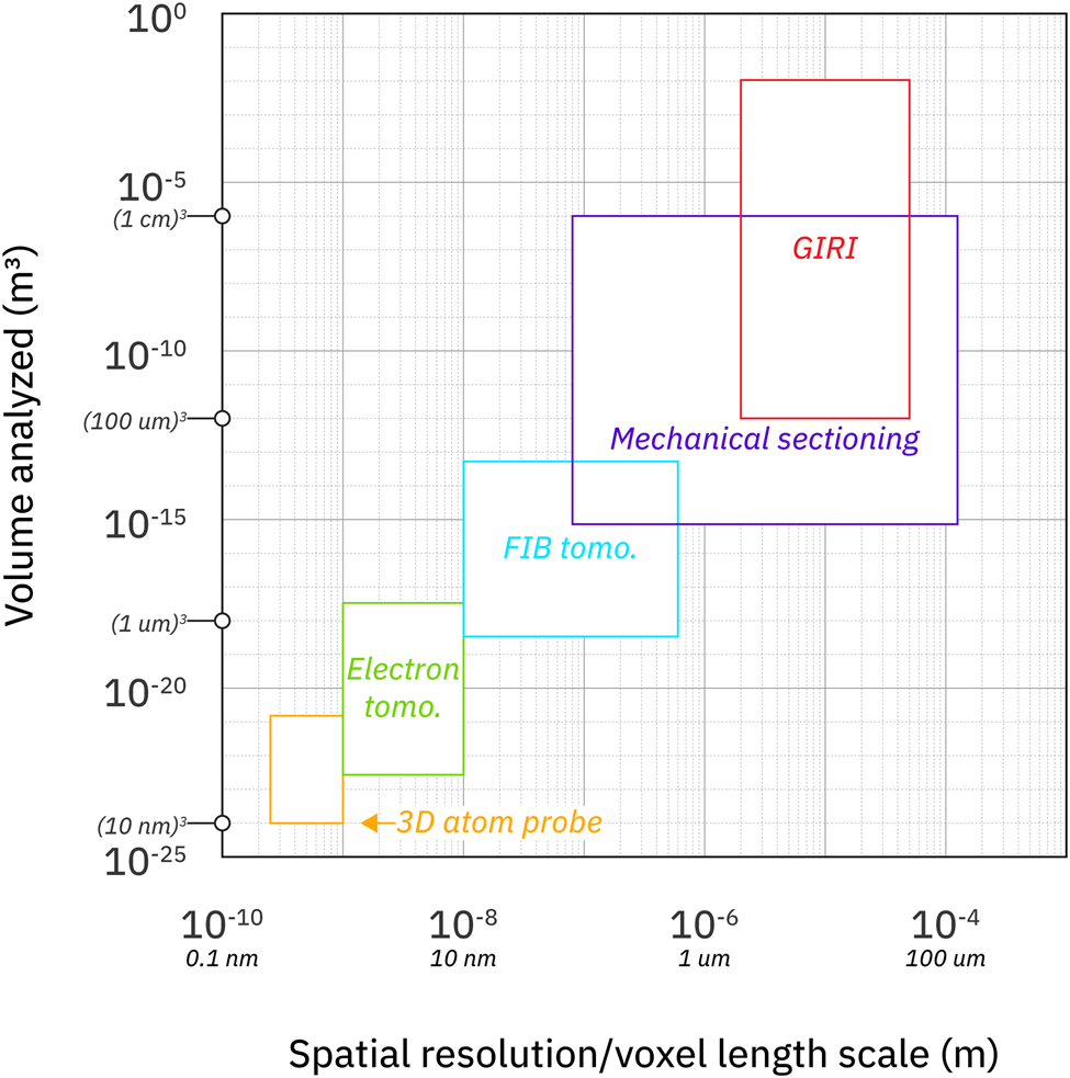
Fig. 1. Resolution versus volume analyzed of various tomographic techniques. GIRI expands the size of mechanically sectioned samples that can be imaged at high resolution (figure adapted from Cantoni & Holzer, Reference Cantoni and Holzer2014). Both axes are log-scale and equivalent SI units are in small italics.
Given the value of 3D data, all tomographic imaging techniques are indispensable and often complementary. For example, X-ray CT is an obvious choice in situations where destruction must be avoided, while optical imagery made with mechanical sectioning is ideal for samples with little to no material or density contrast. In this paper, we focus on serial sectioning as a tool for producing high resolution, large-volume reconstructions, with the intent of acquiring quantitative 3D metrics of samples at a scale and fidelity that cannot be attained with other, existing techniques. To that end, we present a new, automated methodology for serially grinding and imaging. In addition to addressing many shortcomings of previous methods, our technique dramatically increases the scale of sample volumes that can be probed at micron resolution.
The Grinding, Imaging, and Reconstruction Instrument (GIRI) at Princeton University is a one-of-a-kind apparatus that produces micron-scale data over a decimeter-scale field of view with minimal operator intervention. GIRI comprises a Computer Numerical Control (CNC) Mitsui MSG-818PC-NC surface grinder that is retrofitted with a misting apparatus, retractable rollers, and an imaging stage made up of lighting and a reprographic camera. To demonstrate how data from GIRI can be turned into 3D reconstructions, we present a neural network-based image processing pipeline that can, with some user input, rapidly and accurately segment images. We demonstrate GIRI's effectiveness in a series of case studies with novel results.
Background
In 1903, William Sollas, a professor of geology and paleontology at the University of Oxford, presented a paper to the Proceedings of the Royal Society in which he described a newly invented device that enabled researchers to study fossils using serially polished surfaces (Sollas, Reference Sollas VIII1904). The apparatus comprised a mechanical chuck designed to hold a sample and a rotating glass disk that was continuously fed with a combination of water and abrasive media. By incrementally lowering a mounted sample onto the glass disc, a user could both remove material and polish the sample face via mechanical grinding. The user then would either photograph or trace the freshly polished face for later serial reconstruction and analysis. Spacing between successive sections was reported to be as small as 0.25 mm (Sollas, Reference Sollas VIII1904). Until Sollas’ invention, 3D internal analysis of fossils largely had eluded paleontologists. Unlike biologists, who were able to slice specimens into a series of parallel thin (transparent) sections, scientists that studied fossils had to rely on mechanical processes that, at best, required 1 mm spacing between sections (Sollas, Reference Sollas VIII1904).
Sollas’ design has been modified numerous times throughout the 20th and 21st centuries (Jefferies et al., Reference Jefferies, Adams and Miller1962; Keyes, Reference Keyes1962; Hendry et al., Reference Hendry, Rowell and Stanley1963; Sandy, Reference Sandy1989; Alkemper and Voorhees, Reference Alkemper and Voorhees2001; Sutton et al., Reference Sutton, Briggs, Siveter and Siveter2001; Watters & Grotzinger, Reference Watters and Grotzinger2001; Maloof et al., Reference Maloof, Rose, Beach, Samuels, Calmet, Erwin, Poirier, Yao and Simons2010; Pascual-Cebrian et al., Reference Pascual-Cebrian, Hennhöfer and Götz2013), including, within 10 years of his 1904 presentation, by Sollas and his daughter Igerna (Sollas & Sollas, Reference Sollas and Sollas VI1914). Each iteration of the method has had to contend with the same set of operational concerns: (a) resolution, (b) field of view, (c) registration, (d) operation time and effort, and (e) sample destruction. Resolution determines the smallest feature that can be captured accurately; in serial grinding, resolution refers to both the spacing between successive slices and the sampling interval on freshly ground surfaces. Field of view corresponds to how much surface area is captured by imaging or recording; depending on the capture technique, optical distortion may limit how much of the field of view is dimensionally accurate (in both two and three dimensions). Registration describes how slices are aligned; accurate registration is required to avoid spatial distortion in the final reconstruction. Operation time and effort refers to the processes of sample preparation, grinding, and imaging. Finally, sample destruction is a fundamental characteristic of the technique, meaning that serial grinding may not be suitable for especially rare or precious samples.
Often, these operational concerns are interconnected. For example, an increase in sampling resolution (whether accomplished by decreasing the spacing between slices or by altering the imaging setup) can lead to a decrease in the field of view and/or an increase in sample processing time. Some, though not all, factors can be addressed by creative engineering. For instance, to align successive slices, Sollas proposed either shaping samples into parallelopipedons or, for very large objects, inserting cylinders of graphite into pre-drilled holes to serve as registration marks (Sollas, Reference Sollas VIII1904).
A relatively recent commercial example of serial grinding is an automated system known as Robo-Met.3D, which was first described by Spowart et al. (Reference Spowart, Mullens and Puchala2003) and has been sold since 2006. This device utilizes robotic elements for grinding and polishing and an inverted microscope for imaging (Ivanoff & Madison, Reference Ivanoff and Madison2020). Among other applications, Robo-Met.3D has been used to describe microstructures in metals and alloys, identify flaws in additively manufactured parts, and quantify fibers in composite materials. Certain instances of the device have been augmented to provide multimodal analyses, such as the inclusion of a scanning electron microscope (SEM) to produce backscattered-electron (BSE) and electron backscatter diffraction (EBSD) imagery (Chapman et al., Reference Chapman, Uchic, Scott, Shah, Donegan, Shade, Musinski, Obstalecki, Groeber, Menasche and Cox2019). Robo-Met.3D is optimized for small volume reconstructions (e.g., <1 mm3 up to <27 cm3, as according to Ivanoff & Madison, Reference Ivanoff and Madison2020) and, for sufficiently large samples, relies on photo montages made up of tens to hundreds of image tiles that have been stitched together.
Regardless of how serial data are collected, those data must be processed and reduced before they can be analyzed. Data take the form of an evenly spaced grid of cells known, in 2D optical imagery, as pixels (Figs. 2a, 2b). Each pixel contains a numerical value (multispectral images, such as true color photographs, often contain multiple layers, or channels, of pixels, with the final rendered output being some combination of three channels). These values can be differentiated using a process known as segmentation (Figs. 2c, 2d), in which each pixel is assigned to a predefined class (i.e., semantic segmentation) and objects of interest are identified and separated (i.e., instance segmentation). The ultimate goal of segmentation (semantic and/or instance) is to clearly delineate features of interest from their surroundings, thereby streamlining quantitative analyses. In its simplest form, segmentation involves careful manual tracing of features based on visual differences, which is a process that, while effective, is both time-consuming and prone to operator bias. More sophisticated segmentation methods involve computer algorithms that classify on the basis of numerical values. Simple algorithmic implementations of semantic segmentation, such as thresholding or k-means, operate on individual pixels. However, with increased textural variability resulting from high resolution imagery and/or spectral overlap between desired classes (Figs. 2c, 2d), methods that take into account surrounding pixel values are advisable. Such neighborhood-based techniques can provide additional contextual information (e.g., texture) for use in semantic segmentation, and, in turn, compensate for local heterogeneities (Figs. 2d–2g). To identify individual objects within an image, instance segmentation often relies on mathematical morphological operators (e.g., dilation or erosion) and connectivity (i.e., which pixels of a given class are touching one another). Recently, researchers have introduced machine-learning techniques that combine semantic and instance segmentation into a single, automated pipeline (e.g., Kirillov et al., Reference Kirillov, He, Girshick, Rother and Dollár2019). For a more comprehensive introduction to image segmentation, the reader is referred to Pal & Pal (Reference Pal and Pal1993).

Fig. 2. Image processing considerations. (a) True color image of a calcified fragment of Cloudina, an enigmatic Precambrian fossil (Mehra & Maloof, Reference Mehra and Maloof2018), located within a reddish carbonate matrix. The first zoomed-in region demonstrates that such images comprise a grid of pixels; the second zoomed-in region illustrates how each pixel is comprised of multiple channel values (here, red, green, and blue, or R, G, and B, respectively). The white outline illustrates a target segmentation of the image: a clear separation of two “classes” (i.e., fragment and matrix). (b) Comparative histogram of R, G, and B channel values of the two classes defined in a. Each channel in a digital image contains numerical values ranging from 0 to 2n. Here, each channel has a value between 0 and 216. The solid lines represent the R, G, and B values of the matrix, while the dashed lines represent the R, G, and B values of the fragment (i.e., those pixels bounded by the white outline). Note the overlap between the two classes. Such overlap makes image segmentation challenging. (c) Histogram of the first principal component (PC1) of the image in a. The dashed line illustrates a “threshold value.” Pixels in the PC1 image with values greater than the threshold are classified as fragment, while pixels with values less than (or equal to) the threshold are classified as matrix. (d) Image showing the output of thresholding on the PC1 image. A zoomed-in region—which should be classified as only matrix—illustrates the sort of “speckling” that occurs when a naive threshold is applied to classes that have overlapping values. (e) Example of superpixels generated from the image in a. The zoomed-in region demonstrates how such operations enable the calculations of neighborhood statistics (in this case, of the mean and standard deviation of R, G, and B values of each superpixel) for further image processing. (f) Probability map output from a hidden layer neural network, where each superpixel shown in e is assigned a value between 0 and 1, thereby indicating the likelihood that it is part of the fragment class. The network leverages the neighborhood statistics calculated for each superpixel. (g) Final segmentation output, produced using the probability map shown in f. Each superpixel is assigned the class with the highest probability value, resulting in an image that approaches the target segmentation outlined in a. (h) Diagram illustrating how slices are turned into 3D models. (i) A 3D tube. (ii) One planar cross section through the tube. The square grid depicts discrete sampling of the section. Each square can be considered to be a pixel. (iii) The section shown in ii is given a thickness corresponding to the vertical sampling interval. Each extruded pixel is referred to as a voxel. (iv) When multiple sections are stacked and each is given a thickness, a 3D model is formed. (v) Decreased vertical spacing between successive slices improves the fidelity of the resulting 3D model. (vi) Increasing the planar resolution also increases the model's accuracy with respect to the original form. Scalebar in a depicts 0.5 cm.
Following segmentation, 2D slice data must be converted to a composite 3D volume for measurement. In his 1903 paper, Sollas described how a layer of beeswax—with a thickness corresponding to the sampling interval—was laid onto a slice and then cut away to match the sectional contours of features. A complete 3D wax model could be built by stacking successive layers together (Sollas, Reference Sollas VIII1904). Today, such a process is undertaken digitally: the slices are loaded into software and assigned 3D coordinates that correspond to their relative real-world positions. To produce a volume, each section is given a thickness that corresponds to the spacing between two slices (Fig. 2h). The new, 3D pixels are referred to as volumetric pixels, or voxels.
Methodology
Grinding, Imaging, and Reconstruction Instrument (GIRI)
GIRI is located in a laboratory designed to maximize operational accuracy. The grinder is set on an isolated concrete slab that dampens outside vibration. The temperature is kept constant at 19.8 ± 1.5°C in order to limit the expansion or contraction of machine elements. A dehumidifier is programmed to keep the relative humidity at 35% to inhibit rust formation. The laboratory is equipped with both dust and mist collectors and is kept at positive pressure to keep contaminants out.
Surface grinding is accomplished using a Mitsui MSG-818PC-NC CNC surface grinder (Fig. 3). At its core, the Mitsui MSG-818PC-NC comprises a sample-bearing table (Fig. 3a, 2) along with a grinding wheel (Fig. 3a, 3) attached to a variable speed (i.e., 0–6,000 revolutions per minute) spindle. The table moves both longitudinally and transversely while the spindle moves vertically (perhaps counterintuitively, the machine axes for these movements are X, Z, and Y, respectively). Both the speed and step size of movement in all three axes can be set independently and the Mitsui is capable of moving in 1 μm (0.001 mm) increments in any direction. Validation experiments reveal that both the longitudinal and vertical axes are repeatable and precise to within 2 μm (Figs. 4a–4c). The Mitsui MSG-818PC-NC CNC is controlled via Quickset, a proprietary software that runs on an attached Windows computer (Fig. 3a, 4), and can be operated either manually or using G-code, a numerical control language (Kramer et al., Reference Kramer, Proctor and Messina2000). As part of the G-code, dedicated “M-codes” provide the ability to programmatically retrieve machine data, monitor inputs, and switch output relays.
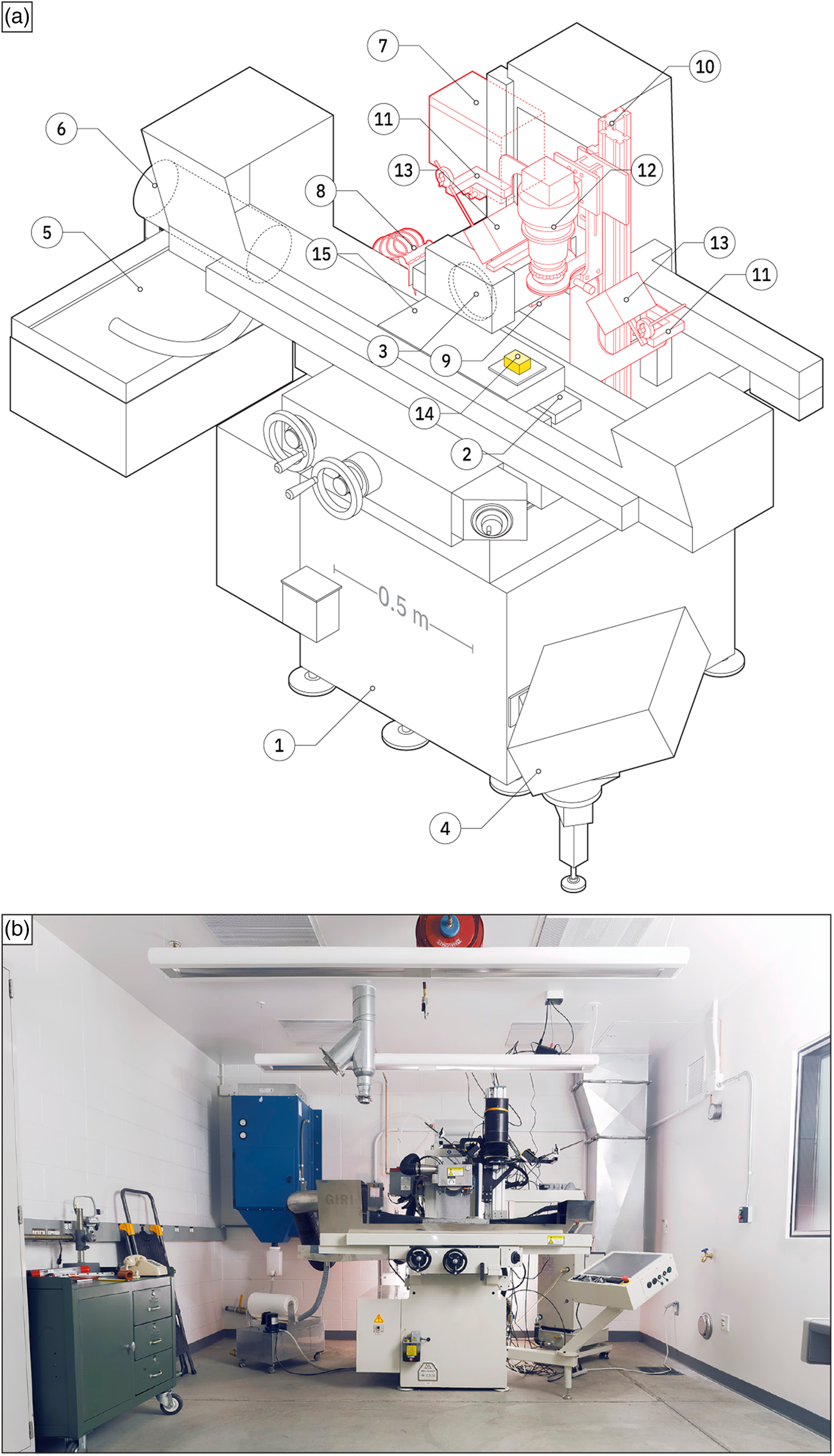
Fig. 3. GIRI elements. (a) An annotated drawing of various elements of GIRI, including: (1) Mitsui MSG-818PC-NC surface grinder; (2) table; (3) grinding wheel; (4) attached Windows computer; (5) coolant holding tank; (6) paper filter roll; (7) misting fluid holding tank; (8) nozzles; (9) retractable roller; (10) vertical rail; (11) arm to hold light(s); (12) reprographic camera system; (13) light; (14) sample, mounted onto a steel plate; and (15) magnetic chuck. Red lines denote retrofitted components. (b) An image of the grinding lab at Princeton University.

Fig. 4. Longitudinal and vertical axis validation experiments. (a) Left: Photograph of an Edmund Optics 50 × 50 mm dot pattern grid image target, where each circle has a diameter of 125 μm. Right: Plot depicting the measured distance between nearest dots as a function of distance from the center of the image. The absence of a trend indicates that the imaging system exhibits negligible distortion. (b) The horizontal positioning of features changes less than one pixel radius over the course of 100 grind cycles. The image target was repeatedly moved out of, then into, imaging position, simulating the table movements associated with each grind cycle. 1,000 circles were identified and tracked across each image. Left, the difference between the center location of each circle between successive images. This plot shows that the MSG-818PC-NC has sub-pixel precision. Right, the difference between the center location of each circle between the first and last image. This plot illustrates that there is no long-term horizontal drift associated with table positioning. (c) Plot showing the difference, in microns, between the prescribed and measured depths of ten steps ground into a single sample (in green and red), along with the results of a simple repeatability experiment, in which the same point on the sample was measured multiple times (termed the “zero measure”; in yellow, with numbers representing multiples of the same value). The depth of each step was measured with a Mitutoyo Absolute Digimatic depth gauge, which has a resolution of 1.27 μm. To explore the repeatability of the gauge, a single point on the ground surface was selected and remeasured a total of 27 times (standard deviation of 1.10 μm). Each step twice was measured in three locations: the left edge, center, and right edge. The average difference across all measures is 0.80 μm. Inset, on the left, a drawing depicting the 10 steps (each 1.5 mm deep) ground into the sample; on the right, a diagram showing how the locations of measurements are arrayed in the plot. Note that darker shades of green indicate multiple measurements with the same value. Scalebar in a depicts 0.1 cm.
Samples are ground using either diamond, silicon carbide, or aluminum oxide wheels of varying grit size. The material properties of a sample, such as hardness, porosity, and/or friability, dictate the selection of wheel material, grit size, spindle speed, and table speed, and many of these grinding parameters have been derived empirically using trial and error. For instance, carbonate rocks—especially those with large lithic grains that are liable to be plucked and drawn over the surface of a sample during grinding—may benefit from the use of aluminum oxide wheels as opposed to the 220–400 grit diamond wheels used for mineralogically hard samples (e.g., granites). At the same time, aluminum oxide wheels tend to wear away faster than diamond wheels, a property that must be accounted for while grinding. To improve surface finish, wheels are manually balanced prior to mounting onto the grinder. Periodically, wheels are trued and dressed, using a brake-controlled truing device for diamond wheels and a single point diamond for silicon carbide and aluminum oxide wheels.
To increase wheel life and improve surface finish, a coolant mixture made up of a water-based synthetic fluid (e.g., Astrogrind A) and deionized water, is directed across both wheel and sample during grinding. The coolant, which is held in a 49.2 L tank (Fig. 3a, 5), is captured and recycled through 10 μm filter media. The filter media comes spooled on a roll (Fig. 3a, 6), which is mechanically unwound and incrementally advanced while the grinder is in operation. As both evaporation and accumulating fine particulate matter slowly alter composition, the depth, pH, hardness, and alkalinity of the coolant are recorded daily and, if necessary, are adjusted by introducing new, dilute coolant.
The Mitsui MSG-818PC-NC is retrofitted with a misting apparatus comprising a 7.5 L holding tank and four, custom-made, independently adjustable combination air and liquid nozzles (Fig. 3a, 7, 8). The misting fluid is made up of a mixture of water soluble oil (e.g., Rustlick WS-11) and deionized water. When actuated, the misting fluid is fed from the holding tank into each nozzle, where it is combined with pressurized air and subsequently atomized over the freshly ground surface of a sample. Misting serves to improve image quality and reduce the appearance of grinder marks (when present). As with other GIRI parameters, the rate and direction of the mist are dictated by specific material properties of a sample. Typically, porous samples, which tend to quickly soak up residual coolant, and larger (i.e., with transverse dimensions exceeding 10 cm) samples, which may undergo uneven drying, require an application of mist, while more impermeable and/or smaller samples do not. Regardless of whether or not misting is employed, excess liquid on the sample surface can negatively impact imaging quality. To address this issue, a retractable roller, which removes any pooled liquid, is attached to the Mitsui MSG-818PC-NC spindle housing (Fig. 3a, 9). The roller, which is made of medium hard (60A durometer) silicone rubber, measures 1.9 cm in diameter, is 15.24 cm long, and is set between two spring-loaded armatures.
An imaging stage is mounted on a vertical rail that is bolted to the table of the Mitsui MSG-818PC-NC (Fig. 3a, 10). The vertical rail moves with the table along the X (transverse) axis. Additionally, the stage is mechanically linked to the spindle housing and, as the grinding wheel is raised or lowered, moves accordingly. To ensure perfect registration between sections, the table is returned to the same Z (longitudinal) coordinate before imaging (Fig. 4b). The imaging stage is made up of two horizontal arms for lighting and a height-adjustable mount for a reprographic camera system (Fig. 3a, 11, 12). Both the lighting and camera system can be upgraded independently of the MSG-818PC-NC, enabling GIRI to take advantage of future advances, including, but not limited to, improved optics, higher spatial or spectral resolution data capture, and/or nonoptical fluorescence (e.g., Manzuk et al., Reference Manzuk, Singh, Mehra, Geyman, Edmonsond and Maloof2022). Typically, lighting is provided by two Lowel Blender adjustable LED lamps (Fig. 3a, 13). The lamps are fitted with polarizing film inserts, which help reduce glare. To leverage sample response to different wavelengths of illumination, multiple Smart Vision LED Brick Lights, each emitting a specific wavelength of light, can be utilized instead (e.g., Manzuk et al., Reference Manzuk, Singh, Mehra, Geyman, Edmonsond and Maloof2022). In such instances, each light is actuated independently via serial communication and multiple photographs (each with exposure times tailored to the specific lighting conditions) are captured (Manzuk et al., Reference Manzuk, Singh, Mehra, Geyman, Edmonsond and Maloof2022). The camera system is a Digital Transitions RCam. The RCam is equipped with an 80 megapixel Phase One digital back that has a camera sensor measuring 4.04 × 5.37 cm and comprising pixels that are each 5.2 × 5.2 μm in size. If utilizing multiple wavelengths of light, the RCam instead is equipped with an achromatic 150 megapixel Phase One digital back, which has a camera sensor measuring 4.04 × 5.37 cm and comprising pixels that are each 3.76 × 3.76 μm in size (Manzuk et al., Reference Manzuk, Singh, Mehra, Geyman, Edmonsond and Maloof2022). Lenses are coupled to the digital back with a Schneider Kreuznach electronic shutter that is controlled using serial commands delivered over USB. The RCam can be fitted with different extension tubes to change the distance from the sensor to lens, enabling the system to utilize multiple focal lengths. Lenses are equipped with a circular polarizing filter to reduce glare and improve image quality. Appropriate working distance for each lens is achieved by moving the camera system up and down a track on the vertical rail. 1:1 macro imaging (corresponding to a resolution of 5.2 μm per pixel with a 4.04 × 5.37 cm field of view for the 80 megapixel back and a resolution of 3.76 μm per pixel with the same field of view for the 150 megapixel back) can be realized using a 120 mm Schneider Kreuznach macro lens, which exhibits negligible distortion from edge to edge (Fig. 4a). Larger fields of view, at the expense of resolution, can be achieved using lenses with shorter focal lengths (e.g., the 72 mm Schneider Kreuznach has a 18.9 × 14.2 cm field of view, with a per-pixel resolution of 18.2 μm on the 80 megapixel digital back). Alternatively, because of the Mitsui's sub-pixel longitudinal precision (Fig. 4b), as well as the distortion-free nature of the Schneider Kreuznach optics (Fig. 4a, inset), samples can be mosaicked and combined to produce large field of view images. The largest imageable area is 26 × 20 cm, while the maximum thickness of a sample is 21.5 cm (a limit dictated by the travel extent of the Mitusi's vertical axis).
An Allen Bradley Micro 830 programmable logic controller (PLC) serves as an intermediate interface between the Mitsui MSG-818PC-NC and a control computer that is located in an adjacent room. Two outputs on the PLC are wired to two inputs on the Mitsui MSG-818PC-NC; conversely, a single input on the PLC is wired to an output on the grinder (Fig. 5). In turn, the PLC is wired to the control computer using a RS232 serial-to-USB connection. The PLC also is connected to a combined temperature and humidity sensor that tracks both parameters over time to ensure that they stay within an acceptable range of values. Furthermore, an acoustic emission grinding sensor (Schmitt Industries SB5560), which can be used to ensure that a consistent amount of material is removed from each cycle, is wired to the PLC (Fig. 5). The data from these sensors are timestamped, stored on the control computer, and regularly backed up to a server on the local network. Via the timestamps, the data can be cross-referenced and used to troubleshoot any issues with the grinding process (e.g., a drop in image quality).

Fig. 5. GIRI schematic. (a) Simplified schematic showing connections between the Mitsui MSG-818PC-NC surface grinder, an Allen Bradley Micro 830 PLC, and a control computer. Italic text refers to operational commands. Arrows indicate the direction of communication. Red lines represent bidirectional data exchange. (b) A table of movement specifications for the Mitsui MSG-818PC-NC. The asterisk refers to the fact that the maximum vertical travel is dependent on the presence of the magnetic chuck (the backslash indicates the range of travel with and without the chuck, respectively).
A collection of custom Matlab scripts allow the control computer to connect and communicate with the PLC, and, in turn, directly interface with the Mitsui MSG-818PC-NC and any associated sensors. Through the Matlab scripts, an operator can: (a) begin a grind cycle, (b) pause and/or resume operation, (c) receive a command to take an image, and (d) activate and/or read from various sensors connected to the PLC. All serial communications, whether sent to or received from the PLC, are archived in digital logs.
Sample Preparation
First, a sample is cut down to size with a circular rock saw. If necessary, the cut-plane orientation, relative to the 3D-geographic orientation of the original sample, is recorded for later reference. Samples that are especially porous and/or friable are vacuum impregnated with epoxy (e.g., Fig. 9d). The sample then is affixed, flat-face down, to a 0.625-cm-thick ground steel plate using two-part epoxy (such as Devcon Two-Ton epoxy adhesive). Although the epoxy begins to harden within five minutes, the assembly is left to cure for 24 h so as to achieve maximum bond strength (Fig. 6a, steps 1 and 2).
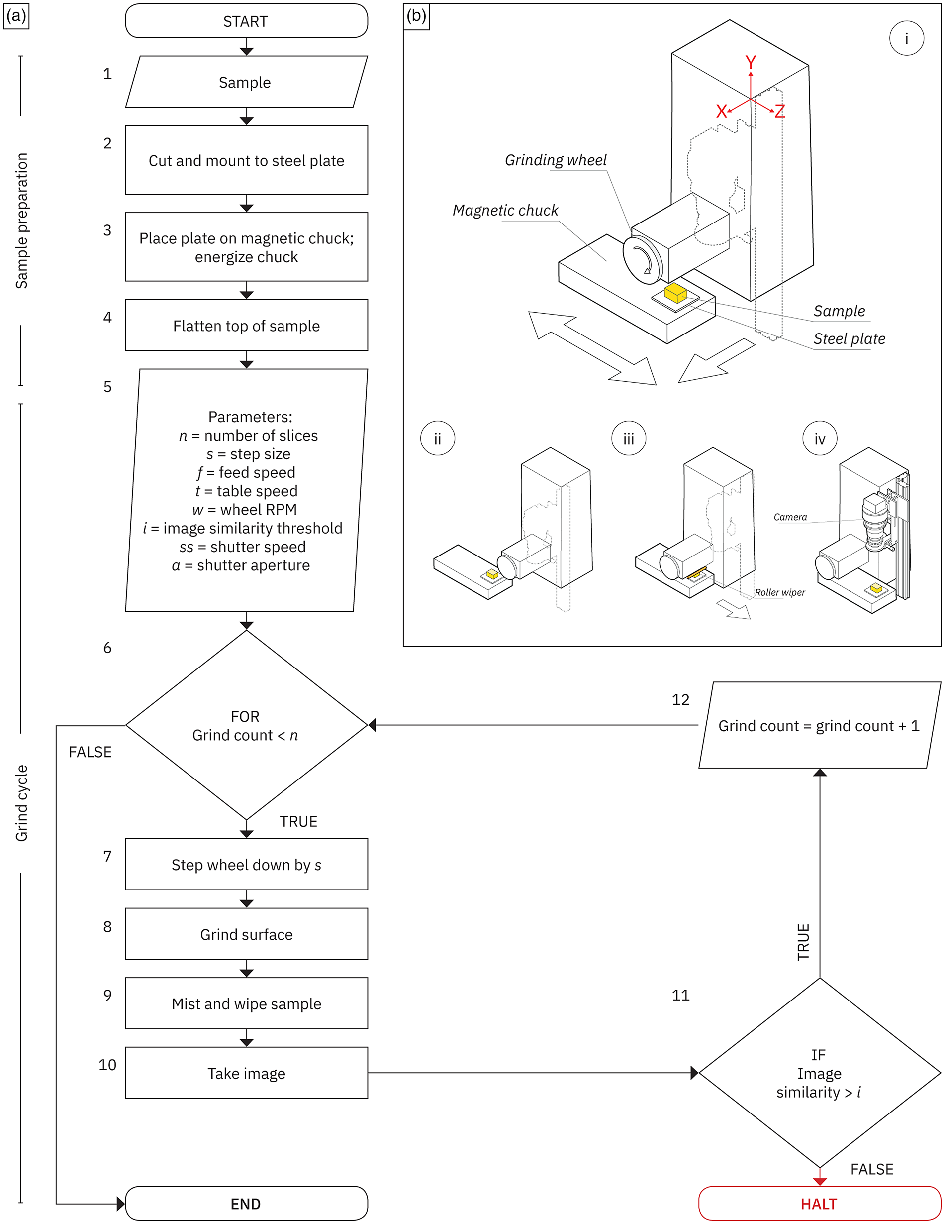
Fig. 6. The grinding procedure. (a) Flowchart depicting each step in the grinding process; steps are numbered on the outside upper left. (b) Diagram illustrating a single cycle of the grinding procedure. (i) Initial position of the sample. Large arrows indicate the direction of table movement. The dashed lines represent the silhouette of the vertical rail and attached camera. (ii) Location of the sample upon completion of surface grinding. If desired, the sample can be coated in mist at this stage of the grind cycle. (iii) Wiping procedure. Large arrow indicates the direction of table movement. (iv) Sample positioned underneath the camera for imaging. The lighting setup is not illustrated.
The steel plate is placed on a manually actuated magnetic chuck (Walker Ceramax 8 × 18; workholding surface dimensions: 20.3 × 45.7 cm; Fig. 3a, 14, 15), which is semi-permanently affixed to the grinder table. The top of the sample then is ground flat by plunge grinding in order to provide an area of adequate flatness and finish for focusing (Fig. 6a, steps 3 and 4).
Camera focus is verified utilizing an iterative procedure. First, Capture One, a software package designed specifically for the Phase One digital back, is used to put the camera into “live view” mode. Next, within the software, three regions on the flattened portion of the sample are identified as “focus areas” for evaluation. For each “focus area,” Capture One uses a proprietary algorithm to produce a graphical output (in the form of a horizontal bar) that visually indicates how well-focused the region is. A fine adjustment screw on the imaging stage—which moves the camera up or down 1/32″ per revolution—then is used to change the camera height relative to the sample, with the intent of maximizing the focus measure for all selected “focus areas.” In practice, the Capture One focus metric maintains its maximum value over a range of approximately two revolutions of the adjustment screw. To dial in the focus at a finer scale, a set of images is captured at 1/4 revolution increments within this two revolution range. The optimal camera height then is determined to be the position at which the image gradient magnitude is maximized. Finally, a test shot is taken to verify visually that the flattened portion of the sample is in focus.
Serial Grinding and Image Acquisition
Several variables are entered into a pre-written G-Code procedure before beginning a grind cycle (Figs. 6a, step 5 and 6b). These variables are: the desired number of grinds (i.e., number of slices), the step size (movement along the Y-axis, in inches), the transverse feed rate (movement along the X-axis, in inches per minute), the longitudinal, reciprocating, table speed (movement along the Z-axis, in inches per minute), and the wheel revolution speed (in revolutions per minute). Separately, a custom Matlab script that interfaces with the shutter controller via serial communication is used to set an initial shutter speed and aperture for the lens. If required, combinations of shutter speed and aperture for multiple exposures (e.g., under different wavelengths of light) also are input at this time. As previously noted, the value for each variable is derived empirically and depends largely on the material properties of the sample being processed. For instance, the typical rotational wheel speed is 3,000 RPM, but this value often is reduced for friable materials. Likewise, while the Mitsui MSG-818PC-NC is capable of moving vertically in 1 μm increments, a step size of either 20 or 30 μm often is chosen as a good compromise between fidelity and the time required for data collection.
Serial grinding commences after all required parameters are set and the camera focus is verified in Capture One. A typical grind cycle begins with the removal of surface material (Fig. 6b, i, ii). First, the grinding wheel is lowered along the Y-axis by the step size, after which the wheel and coolant feed are activated. Next, the table begins reciprocating along the Z-axis. Finally, as it continues to reciprocate, the table is moved along the X-axis so that the sample passes underneath the spinning wheel, thereby grinding down the surface. Once a pass over the entire surface is completed, the wheel, coolant, and table movement are stopped. Optionally, the misting procedure is initiated and the surface is coated with a thin layer of misting fluid. The retractable roller then is actuated and the sample passes below the wiper so as to clear any excess fluid and ensure an even sheen (Fig. 6b, iii). Finally, the sample is positioned under the imaging stage for photographing (Fig. 6b, iv).
The grinder then outputs a signal to the PLC, which in turn tells the control computer to capture an image. The camera and shutter are triggered via Capture One. Upon completing the exposure, Capture One downloads the image and stores it on the control computer. As only slight changes are expected between successive sections, a captured image can be compared to the previous grind's photograph to check for major, undesired deviations in image quality.
A structural similarity algorithm (SSIM) is used for comparison and validation. SSIM determines how similar two photographs (in this case, from the current and previous grind cycles) are on the basis of the luminance, contrast, and signal structure of each image (Wang et al., Reference Wang, Bovik, Sheikh and Simoncelli2004). SSIM produces a single number, which then is compared to a threshold value (typically 0.85, although this value can be adjusted prior to the grind cycle; Fig. 6a, step 5). If the SSIM value is less than the threshold value (or if a capture failed to download), the control computer throws an exception, stops the process, and alerts the operator via text message (Fig. 6a, 11). Phenomena that can result in lower-than-threshold SSIM values include, but are not limited to, changes in lighting (e.g., if one of the LED lamps were to unexpectedly shut off), incorrect sample positioning, or issues with the mechanical grinding process. Once alerted, the operator can address the problem, manually trigger an image capture, and then resume the automated grinding process. This procedure ensures that a valuable sample is not ground away without first creating a viable image archive. In the case of multiple exposures, the Matlab program automatically compares each image to its corresponding photograph from the previous grind cycle and tests the SSIM value against the threshold after every exposure.
If there are no issues with the recorded data, the control computer initiates the next grind cycle by having the PLC input a signal to the Mitsui MSG-818PC-NC. The grinding process then repeats itself. A 1,500 slice sample (at 30 μm per slice for a total thickness of 4.5 cm) takes approximately 5 days to grind and image; during this time, the operator only needs to replace machine fluids and clean the roller once every 24 h.
Image Processing Pipeline
Capture One downloads and stores photographs as .IIQs, a proprietary raw image format that preserves unaltered sensor data. While the raw image data are archived for long-term storage, they must be converted to 16-bit .TIFFs for use in image processing. Exposure, white balance, contrast, and brightness often are adjusted before conversion. The conversion from .IIQ to .TIFF has the downside of increasing image size by an order of magnitude. For example, a single .IIQ file that ranges in size from 50 to 80 MB may have a corresponding .TIFF file that is approximately 600 MB in size. Since individual .TIFFs are so large, it is challenging to load more than several hundred images into memory. Therefore, most processing is done on single images or small groups of images.
Following conversion, one to three representative .TIFFs are selected for use in training. The purpose of training is to identify objects of interest so that an algorithm can “learn” how to differentiate between features within each photograph. The GIRI image processing pipeline utilizes two different neural network architectures for classifying pixels (i.e., semantic segmentation): (a) a hidden layer pattern classification network that relies on an initial oversegmentation using superpixels (clusters of pixels that have similar color and texture values; Fig. 7a), and (b) a convolutional neural network (CNN; Fig. 7b) that segments images using a series of 3D filters. The choice of network is dependent on what features are being segmented. Generally speaking, samples with spatially extensive features of interest (e.g., fossils embedded within a fine matrix) are best for the hidden layer pattern classification network, while samples with finely detailed, texturally distinct—although not necessarily chromatically unique—features (e.g., different mineral phases within a granite) require a CNN.

Fig. 7. Neural networks used for image classification. (a) Schematic diagram of a hidden layer neural network. The input is a vector of numerical values (such as mean R, G, and B color values) calculated from a single superpixel. While the number of hidden layers (n layers) can vary, 50 is a typical value. The number of classes (n classes) is determined by a user prior to training. The output of the network is a list of probabilities—summing to 1—for each class. (b) Schematic diagram of a convolutional neural network. The input is a 33 by 33 pixel neighborhood made up of three (R, G, and B) channels. Following Havaei et al. (Reference Havaei, Davy, Warde-Farley, Biard, Courville, Bengio, Pal, Jodoin and Larochelle2017), the network takes advantage of two different scales of information by splitting into “global” and “local” pathways, each with a different number and size of convolutions. The two pathways are merged before classification.
The training procedure differs based on what neural network architecture is chosen. For the pattern classification network, the first step is to produce n superpixels for each training image utilizing the SLIC algorithm (Achanta et al., Reference Achanta, Shaji, Smith, Lucchi, Fua and Süsstrunk2012). Then, using a graphical user interface written in Matlab, a researcher assigns superpixels to different classes via clicking on individual regions. Finally, statistics for each class (including mean red, green, and blue values, covariance between the different channels, and entropy, which is a measure of texture) are compiled and then used for network training via backpropagation (Fig. 8, steps 5B–D). For the CNN, a researcher identifies and paints pixels associated with specific features in an image editing and/or analysis program such as Adobe Photoshop, GIMP, or Dragonfly. Each pixel within a painted region serves as a representative pixel for that class. The network training is done in Matlab, once again using backpropagation (Fig. 8, steps 5B–D).
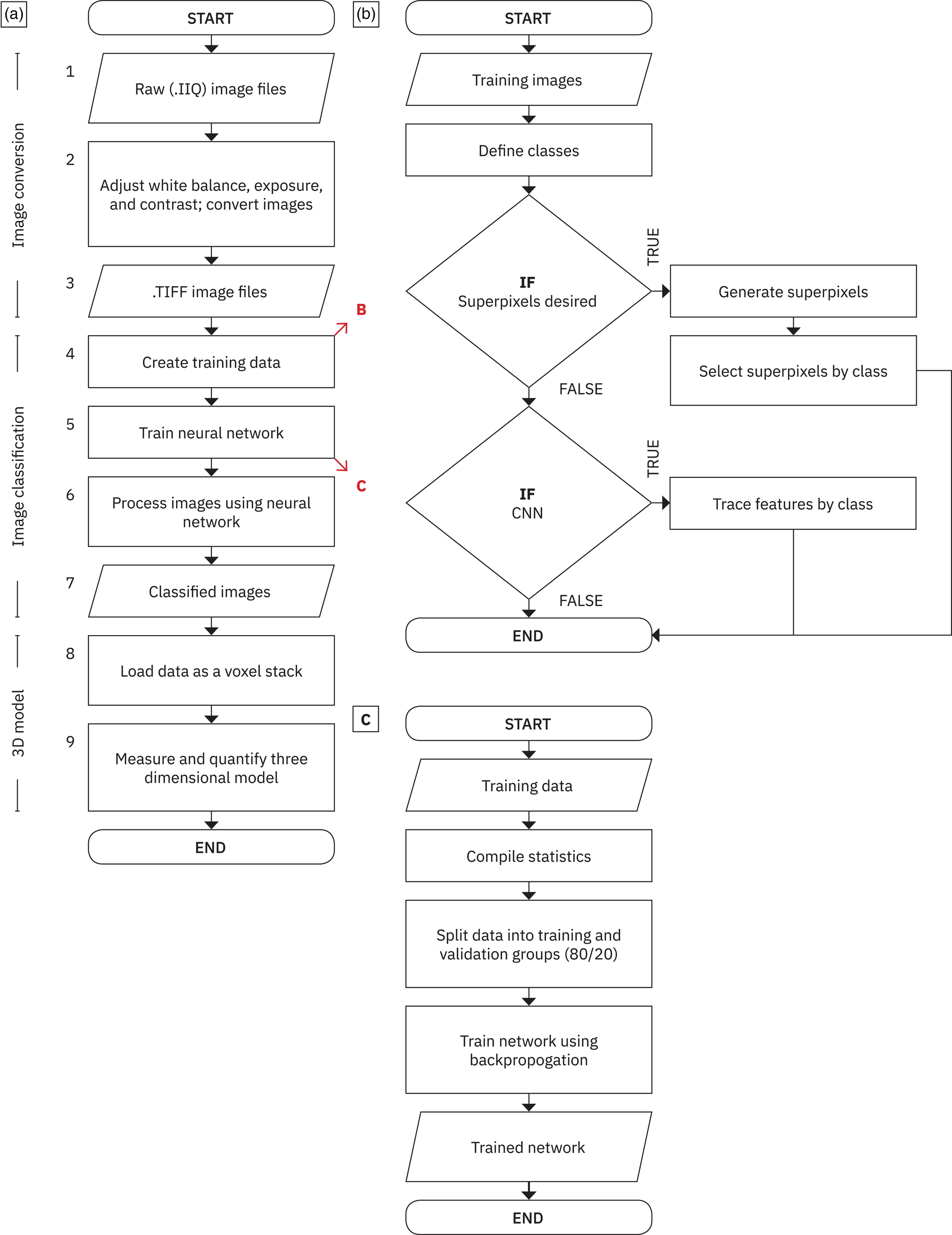
Fig. 8. Image processing procedures. (a) Flowchart illustrating a generalized process for turning raw image data into a 3D model for quantification; steps are numbered on the outside upper left. The red diagonal arrows with letters refer to the sub-procedures detailed in b and c. (b) Procedure for generating training data. (c) Procedure for training a neural network for segmentation. Essential to neural network training is the backpropogation algorithm. Backpropagation updates weights and biases (which are initialized randomly at the start of training) by first propagating inputs through the network, then computing an error metric, then propagating sensitivities (i.e., calculating the relative contribution of an element to the output) back through the network, and finally, using those sensitivities to update each element proportionally (Hagan et al., Reference Hagan, Demuth and Beale1996).
Following network training, the entire image stack is processed, one image at a time, with a forward pass through the trained neural network of choice. Both a probability map—which indicates the network's confidence that a pixel (or superpixel) belongs to a given class—for each class and a final classified .TIFF—which contains a single class value for each pixel—are output and stored (Figs. 2f and 2g, respectively). The classified .TIFFs then can be loaded into any 3D visualization software for measurement and analysis.
Results
Here, we present three case studies, each comprising a real-world example, a description of the morphological properties of interest, the results of various 2D and small-volume reconstruction experiments, and, finally, the analysis made with GIRI. Although these case studies deal with specific geologic materials, the morphological properties—along with the experiments—are generalizable, and applicable to a wide variety of scientific questions.
Shape Metrics of Objects and Porosity Granular Materials
Oolites are sedimentary rocks made up of laminated, ellipsoidal-to-spherical calcium carbonate grains known as ooids, which typically have diameters of less than 0.5 mm (although anomalously large “giant ooids” can grow to be over 2 mm in diameter). Oolites can serve as paleoenvironmental indicators (Bathurst, Reference Bathurst1972; Howes et al., Reference Howes, Mehra and Maloof2021) and hydrocarbon reservoir rocks (Lucia, Reference Lucia1995). The fluid storage capacity of an oolite is controlled by its porosity (i.e., the volume of void space divided by the total volume of a sample) and permeability. These parameters, which effectively describe the void spaces of a sample, are dependent upon the shape, size, and distribution of the solid fraction of a volume. In oolites, porosity and permeability can vary both spatially and temporally: hydrodynamic and biological forces can lead to local heterogeneities within the rock (e.g., grains sorted by wave action or burrows made by animals) while, over time, the precipitation of new calcium carbonate cements and/or the dissolution of existing grains and cements can change void spaces and interconnectivity. To accurately estimate porosity and permeability values, it is necessary to identify and segment both the grains and the multiple generations of cement that make up an aggregate. Once isolated, spatial statistics of the original grains can help constrain paleoenvironment, while morphological descriptions of both the cements and void spaces can aid estimates of the evolution of paleo-fluid migration and storage.
Small volume (e.g., millimeter scale) reconstructions can lead to inaccurate estimates of both porosity and permeability. For example, in the case of a Holocene oolite from Joulters’ Cay, Andros Island (Figs. 9a, 9b), porosity values measured from a 1 mm3 subvolume of the oolite can vary by up to 23%; this variation drops to 4.7% when examining 0.343 cm3 volumes (Fig. 9c). Estimates of absolute permeability, calculated using OpenPNM (Gostick et al., Reference Gostick, Aghighi, Hinebaugh, Tranter, Hoeh, Day, Spellacy, Sharqawy, Bazylak, Burns, Lehnert and Putz2016), span five orders of magnitude when looking at 1 mm3 subvolumes of the oolite (25th/50th/75th percentiles of 100 randomly drawn volumes: 714.5/2110.4/4411.2 mD; Fig. 9d). This variation is reduced with larger (i.e., 0.343 cm3) volumes, where the estimated permeability (25th/50th/75th percentiles of 100 randomly drawn volumes: 108.0/310.0/659.8.2 mD) is consistent with values reported for reservoir rocks (Bear, Reference Bear1988). Estimates of permeability and porosity made on small volumes will be especially bad for granular materials with very large grains. In the case of an Early Triassic oolite from the Great Bank of Guizhou in South China (Howes et al., Reference Howes, Mehra and Maloof2021), which contains so-called giant ooids, the median maximum Feret diameter of individual ooids is 4.4 mm (25th/75th percentiles: 3.7/5.5 mm). Therefore, a 1 mm3 volume would be too small to image a single ooid, precluding any accurate estimate of porosity or permeability.

Fig. 9. Oolite case study. (a) Slice through an oolite from Joulters’ Cay, Andros Island, the Bahamas. Ooids are white. The blue color is a result of epoxy impregnation, which is necessary because the sample is weakly cemented. Inset: a thin section image of the same oolite, illustrating the ooids, cements, and pores that make up the sample. (b) Three-dimensional reconstruction of the sample shown in a. (c) Porosity (volume of void over total volume; in percent) as measured on random subvolumes of the reconstruction shown in b. Three different sizes of subvolumes are used; as volume increases, the variability decreases. The porosity value for the entire volume shown in b is marked by the red dashed line. (d) A plot depicting permeability (in mD) values measured on random subvolumes of the reconstruction shown in b. Permeability values were calculated using OpenPNM (Gostick et al., Reference Gostick, Aghighi, Hinebaugh, Tranter, Hoeh, Day, Spellacy, Sharqawy, Bazylak, Burns, Lehnert and Putz2016). The calculated permeability value for the volume shown in b is depicted by the red dashed line. Scalebars in a and b depict 0.5 cm.
It is important to note that, due to a clear density contrast between solid and void space, modern oolites are excellent candidates for reconstruction via X-ray CT. However, even young rocks contain some amount of secondary cementation, which—owing to similar mineralogical and chemical properties between grains and cements (Fig. 9a)—may not be differentiated via X-ray CT, leading to measurement error. This problem only is compounded as primary void spaces are, over time, progressively filled with cement and/or sediment. Additionally, X-ray CT cannot distinguish between different growth rings in individual ooids (again, because there is no phase or density difference), which is an integral aspect of piecing together paleoenvironments (Howes et al., Reference Howes, Mehra and Maloof2021) or changes in primary and secondary porosity and/or permeability. For such applications, reconstructions based on optical imagery (acquired via serial grinding and imaging) are required.
Modal Makeup of Irregularly Shaped, Interlocking Crystals
We now turn to materials made up of interlocking crystals, where there is a need to better understand the size, shape, and concentration of each crystal. To date, complete and accurate morphological descriptions of crystals within granites (or other igneous rocks), which are required to produce and evaluate true crystal size distributions (CSDs), remain elusive. Often, CSDs are made using stereological corrections, which rely on a set of geometric assumptions (such as modeling minerals and bubbles as spheres; Armienti, Reference Armienti2008). Complementary to CSDs are modal analyses, which provide an accounting of the proportions of different minerals within a rock. Such analyses are accomplished by using either point counting (Neilson & Brockman, Reference Neilson and Brockman1977) on 2D thin sections or model estimates from whole rock geochemistry. Serial sectioning opens up the possibility of making 3D CSD and modal analyses. However, when individual crystals are millimeter scale, large volumes are required to produce reliable estimates of either CSD or modal mineralogy. For instance, when calculating the relative proportions of four different mineral phases within a granite, values do not converge in volumes smaller than 1 cm3 (Figs. 10a, 10b). Estimates of modal mineralogy can be up to 20% wrong even when averaging over multiple cm3 volumes (Fig. 10c).

Fig. 10. Granite case study. (a) Diagram illustrating three subvolume sizes: 1 mm3, 125 mm3, and 1 cm3. (b) Evolution of modal mineralogy as a progressively larger subvolume (growing from the center of the granite volume shown in a and f) is measured. Black arrows on the right of the figure depict the modal mineralogy for the entire volume. Estimates of modal mineralogy from mm3 volumes of crystalline rocks can be inaccurate. (c) Histograms showing that errors in estimates of modal proportion may persist even as increasing numbers of successive subvolumes are averaged together. For each size shown in a, 1, 2, and 5 samples are repeatedly (100 times) extracted and an average proportion for each phase is calculated. These averaged values then are subtracted from the true, known values, and the resulting error values are plotted as histograms. While taking a large number of subvolumes does lead to a smaller range of error, accuracy is predominantly controlled by volume size. (e) Slice through a granite from the Golden Horn Pluton. (f) Classified 3D granite volume. (g) Ternary showing the relative proportions of albite, orthoclase, and quartz. In order to plot the three phases shown in the ternary, the plagioclase volume is split into albite and anorthite using whole rock measurements of calcium to calculate the relative proportion of each phase. Inset left, graph illustrating how the mean relative proportions varies as each slice is measured, suggesting that there is a minimum volume that must be measured before acceptable results are attained. Inset right, box plot showing the wide range of relative proportions measured on each (individual) slice of the granite. Scalebars in e and f depict 0.5 cm.
The Eocene Golden Horn batholith in the North Cascades, Washington is a fossilized magma chamber in which hypotheses of high silica melt formation can be tested using 3D models made with GIRI. Granites from the Golden Horn can be segmented into four mineral phases: plagioclase, potassium feldspar, quartz, and “mafics” (an all-encompassing designation that incorporates biotite and hornblende, among other dark minerals). Modal analyses, calculated as a first step toward producing true 3D CSD of granites, reveal that the proportions of albite, orthoclase, and quartz (normalized to the sum of their volumes) are 45, 25, and 30%, respectively (Figs. 10e–10g). These values are comparable to modal values derived from large volume (0.3 m3) whole rock geochemical analyses. As the latter are model estimates—made with computed mineralogy (i.e., using the CIPW norm, which calculates the mineralogy of anhydrous magmas, to arrive at a final mineral composition, e.g., Kelsey, Reference Kelsey1965) and projection schemes with empirical corrections (Blundy & Cashman, Reference Blundy and Cashman2001)—an exact match should not be expected. Our reconstruction can be used to produce true 3D CSD, which then can be compared to other granite samples from the Golden Horn batholith. The presence or absence of size and/or geochemical trends within the resulting dataset can reveal whether settling and/or compaction occurred within the system, constraining how magma bodies (such as those under Yellowstone National Park) form and evolve.
Angles and Geometry of Pseudomorphs
Minerals are made up of repeating atom-scale lattices that impart specific symmetries, morphologies, and patterns of fracture to crystal forms. With pseudomorphs—crystals that retain the original shape, but not the chemistry or structure, of a mineral—the size of interfacial angles and description of axes of symmetry can be used to identify the precursor mineral. The correct identification of a pseudomorph can provide insight into the environmental conditions that existed at the time of crystalization. For example, cherts from the Barberton Greenstone Belt contain a pseduomorph that is purported to be after gypsum. It is proposed that the gypsum crystals formed within deep water sediments (de Wit & Furnes, Reference de Wit and Furnes2016). Pointing to the fact that, in the modern, the arrival of cold bottom waters to continental shelves in the North and South Atlantic result in gypsum crystal growth, researchers have used the presence of the pseudomorphs after gypsum to argue that Archaen ocean waters must have been cold (de Wit & Furnes, Reference de Wit and Furnes2016). Such cold waters would suggest that Earth had a cool climate 3.4 billion years ago. This hypothesis is controversial, as studies of oxygen and silicon isotopes have inferred that Earth's surface and oceans were extremely hot (e.g., 60–80°C) at the time (Knauth & Lowe, Reference Knauth and Lowe2003; Robert & Chaussidon, Reference Robert and Chaussidon2006).
When studying pseudomorphs, 2D cross-sections may not preserve the correct number of sides of a crystal or the true angles between those sides, leading to an incorrect determination of symmetry as well as crystal habit (Figs. 11a–11c). For example, out of 9,181 random 2D slices through a hexagonal crystal with sixfold symmetry, only 59% of the cross-sections exhibit six sides. Additionally, not every six-sided cross section is a regular hexagon (i.e., each internal angle measuring 120° and the sum of angles being 720°; Fig. 11c), thereby precluding an accurate reconstruction of symmetry, and, in turn, the original form.

Fig. 11. Pseudomorphs case study. (a) A hexagonal volume with four random cross sections. (b) The cross sections shown in a with their respective number of sides (top text), axes of symmetry (black dashed lines), and rotational symmetry specification (bottom text) notated. Note how it is possible to produce a hexagonal cross section with no axes of symmetry. (c) Histogram showing the angles measured on 9,181 cross sections through the hexagonal volume. Colors correspond to the number of sides in each cross section. The inset pie chart illustrates how often a shape with n sides appeared. The colored vertical lines show the expected angle value for a regular polygon with n sides. (d) Slice through a pseudomorph-bearing sample from the Barberton Greenstone Belt. (e) Model of a single, seemingly hexagonal crystal, with oriented cross sections in red. (f) Model of a single crystal that exhibits twinning. (g) Top, a single section through the crystal shown in e. Internal angles demonstrate that the section is not a regular hexagon. A 180° rotation is shown in dashed lines, illustrating that the section has twofold symmetry. No mirror planes can be identified. Bottom, three sections, ordered from top to bottom, through the crystal shown in f. The formation of twins can be seen in the second and third cross sections. The dotted line depicts the twin plane. Scalebars in d, e, and f depict 0.5 cm.
3D models of pseudomorphs (Figs. 11d–11g) reveal that cross sections—made perpendicular to the long axes of the crystals—have six sides. These hexagonal cross sections are not regular, lack clear mirror planes, and exhibit a twofold symmetry (Fig. 11g). By themselves, the cross sections are not diagnostic of any one mineral (e.g., both aragonite and gypsum exhibit similar pseudohexagonal forms). However, the reconstruction of a macroscopic centimeter-scale twinned crystal, with swallowtail twins on the 001 plane (Figs. 11f, 11g, bottom; Hurlbut and Klein, Reference Hurlbut and Klein1977), suggests that the pseudomorphs are, in fact, after gypsum.
3D Reconstructions of Large Volumes Both Extend and Complement Existing Analytical Methods
Automated mechanical serial sectioning is a well-established technique for generating 3D reconstructions of objects with low material contrast. GIRI extends the maximum volume (from 27 cm3 to an upper limit of 11,000 cm3) that can be imaged using mechanical serial sectioning (and does so while maintaining image quality, repeatability, and time efficiency). This extension is important because, as our case studies demonstrate, cm3-scale 3D reconstructions can provide critical information that might be missed by 2D or mm3 analyses of materials ranging from granular media to individual, macroscopic objects such as crystals. GIRI's large volume capabilities complement other tomographic techniques, which might present certain advantages, such as higher resolution (e.g., RoboMet.3D or FIB Tomo, Fig. 1), in situ observation (e.g., 4D X-ray CT, where the same volume is imaged over the course of an experiment), or nondestructive data collection (e.g., ultrasound or X-ray CT).
Concluding Remarks
The case studies in this paper provide only a limited illustration of GIRI's reconstruction capabilities. Our serial grinding and imaging technique can address questions in many different disciplines, from geology to material sciences to manufacturing. GIRI is of particular value to the analysis of heterogeneous phenomena, such as fracture networks, size or shape sorting, and permeability, whose properties might greatly vary over small (e.g., mm to cm) distances and which therefore can benefit from the large sample volumes that GIRI can image. Importantly, GIRI is an adaptable and extensible platform that, in the future, could see the addition of a variety of data capture technologies (e.g., Raman, XRF, and/or enhanced multispectral imaging) as required by researchers.
Acknowledgments
We thank F. Maehr and K. Kellerson at Millenium Machinery for helping design, fabricate, install, and troubleshoot GIRI. P. Siegel was instrumental in helping design the imaging stage. At Situ Studio, B. Girit, A. Lukyanov-Cherny, and W. Rozen played fundamental roles in the design and development of GIRI. We thank the late M. De Wit for providing us with the Barberton sample. B. Ferdowsi gave assistance with creating Voronoi packings for synthetic study. This paper benefited from discussions with M. Eddy, B. Ferdowsi, S. Maclennan, and T. Senden. This work was supported by NSF EAR 1028768 to A.C.M and funding from the Princeton Tuttle Invertebrate Fund.


 Open access