


Introduction
X-ray microcomputed tomography ( $\mu$-CT) is an established and indispensable tool to unveil the structure and composition of disordered and inhomogeneous materials (Kinney et al., Reference Kinney, Johnson, Bonse, Nichols, Saroyan, Nusshardt, Pahl and Brase1988; Banhart, Reference Banhart2008; Stock, Reference Stock2019). Despite the successful application of $\mu$-CT, there is a class of materials for which it is highly challenging to capture the degree of disorder and to determine the extent of microstructural heterogeneity in general. This class comprises thin sheet materials with enormous aspect ratios. Such materials occur, e.g., in batteries or fuel cells, where $\mu$-CT was successfully used to investigate their local microstructure variations (Harris & Chiu, Reference Harris and Chiu2015; Banerjee et al., Reference Banerjee, Hinebaugh, Liu, Yip, Ge and Bazylak2016). Furthermore, thin sheet materials appear in filtering applications and even as consumer products in daily use. Paper sheets also fall in this class and illustrate well large aspect ratios, as paper features areas in square centimeters or even square meters while it is only several micrometers thin or even less. Correspondingly, possible microstructure variations manifest themselves on length scales that may span seven orders of magnitude (Chinga-Carrasco, Reference Chinga-Carrasco2009). Thus, paper can be considered as a multi-scale material (Kent, Reference Kent1991; Vernhes et al., Reference Vernhes, Bloch, Mercier, Blayo and Pineaux2008; Simon, Reference Simon2020), particularly when variations in transversal and lateral directions are compared. The quantification of microstructure variations in both directions, i.e., variations on two different length scales, is crucial to predict the macroscopic behavior of paper sheets and of thin sheet materials in general. Using $\mu$-CT allows for resolving features on the sub-micrometer scale. Still, it practically limits the field of view captured with a single $\mu$-CT scan, which is several orders of magnitude smaller than the required lateral extension. Hence, it is highly desirable to explore how $\mu$-CT can be utilized in combination with statistical image analysis to characterize microstructures of such high aspect ratio materials, including their local variations. In the present study, we consider paper-based materials and their pore space as an elegant test bed for designing and performing a $\mu$-CT-based microstructure acquisition that is capable of revealing variations that laterally occur within a sheet. In general, paper materials consist of a complex network of fibers. When paper sheets form, the fibers tend to arrange into mats being one fiber thick that stack on top of each other. This forming process induces strong local variations in the microstructure of paper, which are typical for fiber-based microstructures in general (Dirrenberger et al., Reference Dirrenberger, Forest and Jeulin2014). The microstructure, in turn, strongly influences the effective macroscopic properties of paper. Thus, a quantitative understanding of relationships between the microstructure and effective macroscopic properties, as, e.g., the air permeance (Gurnagul et al., Reference Gurnagul, Shallhorn, Omholt and Miles2009), must account for these local variations.
For paper sheets, lateral mapping of locally varying properties such as thickness, basis weight, and transversally averaged mass density was already demonstrated (Dodson et al., Reference Dodson, Oba and Sampson2001a, Reference Dodson, Oba and Sampson2001b; Sung et al., Reference Sung, Ham, Kwon, Lee and Keller2005; Sung & Keller, Reference Sung and Keller2008; Keller et al., Reference Keller, Branca and Kwon2012). Such studies readily combine a lateral resolution as low as 100  $\mu$m with mapped areas of 25–100 mm $^{2}$ (Keller et al., Reference Keller, Branca and Kwon2012). To achieve mass density maps, $\beta$-radiography for basis weight determination is combined with laser profilometry for thickness mapping. Though already correlations between local thickness and basis weight can be elegantly extracted from these maps (Dodson et al., Reference Dodson, Oba and Sampson2001a; Keller et al., Reference Keller, Branca and Kwon2012), it is highly desirable to also incorporate details of the pore space, e.g., to establish relations between basis weight, thickness, and porosity (Dodson & Sampson, Reference Dodson and Sampson1999).
For properties associated with the pore space of paper, the impact of local variations on the so-called floc scale is not well established so far. Flocs are regions in which the fibers tend to aggregate more strongly than in adjacent regions and are non-regularly distributed across the paper sheets. Size and separation of such flocs can continuously vary between several micrometers and centimeters. Previous studies employing  $\mu$-CT scans intriguingly indicate that selected properties associated with the porous nature of the microstructure can be reliably captured with representative elementary volumes (REVs), see Rolland du Roscoat et al. (Reference Rolland du Roscoat, Decain, Thibault, Geindreau and Bloch2007, Reference Rolland du Roscoat, Bloch and Caulet2012), Defrenne et al. (Reference Defrenne, Zhdankin, Ramanna, Ramaswamy and Ramarao2017), and Aslannejad & Hassanizadeh (Reference Aslannejad and Hassanizadeh2017). Note that beside 3D imaging, synthetic microstructures modeling paper sheets are used to quantify REV sizes (Li et al., Reference Li, Yu, Reese and Simon2018). Such an REV, as defined in Kanit et al. (Reference Kanit, Forest, Galliet, Mounoury and Jeulin2003), is the smallest volume cutout from which certain (global) microstructure descriptors can be computed with a pre-defined accuracy. This pre-defined accuracy influences the REV size, see the detailed discussion in Section 5.2 of Rolland du Roscoat et al. (Reference Rolland du Roscoat, Decain, Thibault, Geindreau and Bloch2007). This means, in turn, that for a given REV size, the variability of microstructure descriptors does not completely vanish. Note that, instead of one large volume, a sufficiently large number of small volumes can be considered as representative for a given microstructure (Kanit et al., Reference Kanit, Forest, Galliet, Mounoury and Jeulin2003). Further investigations of REV sizes in the spirit of Kanit et al. (Reference Kanit, Forest, Galliet, Mounoury and Jeulin2003) can be found, e.g., in Fritzen & Boehlke (Reference Fritzen and Boehlke2011) for metal ceramic composites, in Stroeven et al. (Reference Stroeven, Askes and Sluys2004) for granular materials, or in Wimmer et al. (Reference Wimmer, Stier, Simon and Reese2016) for asphalt concrete.
In the present study, we go beyond the investigation of REV sizes and quantify local variations of microstructure descriptors in regions, which are smaller than the REV size. Moreover, we propose a  $\mu$-CT-based workflow to acquire sufficiently large and highly resolved image data of the microstructure to incorporate the floc scale, i.e., to reach out to variations that laterally occur within the sheet. For that purpose, we use model paper sheets with marked variations in the local basis weight. These variations are present not only at length scales accessible with submicrometer-resolved $\mu$-CT scans, but also beyond a centimeter, i.e., at the floc scale. To check whether the resulting data set is large enough to capture the local variations on the floc scale, we applied our workflow to a model paper before and after hard-nip calendering. The calendering technique is abundant in paper making and compresses the paper to smooth its surfaces. In our case, we use hard-nip calendering to modify the microstructure of paper sheets and its variation in a controlled way. As the model paper contains virgin fibers without additional fillers or coating, the calendering transforms local variations of the sheet thickness into local variations of the corresponding mass density (Sung et al., Reference Sung, Ham, Kwon, Lee and Keller2005). Along with a local densification, the surface roughness is also reduced. This is an effect, which has been elucidated in Sampson & Wang (Reference Sampson and Wang2020) based on theoretical considerations and supported by a data-based validation. Regions notably rich in fibers (flocs) are densified, while regions with fewer fibers (i.e., regions with a small local thickness) remain practically unchanged. Hence, calendering is expected to cause changes regarding local variations of pore space-related properties. If the image data obtained by $\mu$-CT and related to the uncompressed and compressed paper are sufficiently comprehensive, we should be able to reveal and explain the impact of the transition on the local porosity, thickness, and pathways through the pore space. Thus, based on our previously published approach for the statistical analysis of local variations in the microstructure of paper materials (Neumann et al., Reference Neumann, Machado Charry, Zojer and Schmidt2021), we will quantify the local variations of porosity and path length-related descriptors as well as the correlation between these quantities. Moreover, in the present study, we will also take into account an additional structural descriptor, namely the local thickness of the considered paper sheets.
The remaining part of the present article is structured as follows: first, we give a methodological overview, which includes descriptions of the materials and experimental measurements, the workflow to efficiently perform  $\mu$-CT scans for providing a comprehensive set of image data representing the microstructure, and a description of the methods used for statistical image analysis. Second, we quantify the influence on the paper materials induced by compression. We present results regarding experimentally determined macroscopic characteristics and results regarding changes in the microstructure obtained by statistical image analysis. In particular, methods of statistical image analysis are used to reveal whether the changes in the microstructure due to local compression can be unambiguously identified and explained. This is done on the basis of analyzing the (univariate) distribution of local structural descriptors of the pore space and of pairwise correlations between them. Moreover, we scrutinize the representativity of our data sets, i.e., we analyze the dependence of our results on the size of image data.
Materials and Methods
Material and Experimental Characterization
As a model system for our investigations, we consider the same paper material before and after compression. As an uncompressed reference material, we use a commercial, unbleached paper with a specific basis weight of 100 g/m $^{2}$. This value, which corresponds to the supplier specifications, was confirmed by a test in accordance to the corresponding ISO standard (ISO 536:2019, 2019). The paper consists of virgin fibers, does not contain intentional fillers, and has not passed any mechanical post-treatment. During the forming of such a paper, any local accumulation of fibers (flocs) leads to thickness variations in the sheet. Though these thickness variations are induced by local variations in the basis weight, the local mass density ought to show small deviations only. For obtaining compressed samples, several sheets of the reference paper were subjected to a hard-nip, steel–steel calendering with a line load of 90 N/m.
Each paper type underwent a basis characterization in terms of basis weight, caliper-based thickness, smoothness, and air retention times. The local basis weight was determined using  $\beta$-radiography as described in Kritzinger et al. (Reference Kritzinger, Hirn, Donoser and Bauer2008). Note that smoothness and retention times have been determined with the Bekk method (ISO 5627:1995, 1995) and the Gurley method (ISO 5636-5:2013, 2013), respectively.
Workflow to Acquire Large  $\mu$-CT Data Sets

3D imaging via  $\mu$-CT is an established method to explore the pore space of paper (Rolland du Roscoat et al., Reference Rolland du Roscoat, Decain, Thibault, Geindreau and Bloch2007, Reference Rolland du Roscoat, Bloch and Caulet2012; Aslannejad & Hassanizadeh, Reference Aslannejad and Hassanizadeh2017; Defrenne et al., Reference Defrenne, Zhdankin, Ramanna, Ramaswamy and Ramarao2017). When focusing on the pore space, the large spread of pore sizes requires a particularly balanced trade-off between resolution and field of view, i.e., the sample size. A high resolution aids to reveal smaller pores with diameters in the range of 1 $\mu {\rm m}$. Such an appropriate voxel resolution of 0.7 $\mu {\rm m}$ permits to scan a volume of approximately $2\, {\rm mm}^{2} \times {\rm thickness}$.
In such small volumes, it is challenging to capture a representative amount of larger pores with diameters in the order of 50  $\mu {\rm m}$ and beyond. The above-mentioned sample volume of approximately $2\, {\rm mm}^{2} \times {\rm thickness}$ is particularly small in comparison to fields of view in the 1–10 cm2 range that are considered to capture local variations including the floc scale (Sampson, Reference Sampson2001). To explore the microstructure of paper materials beyond these small volumes without sacrificing resolution, multiple sample volumes stemming from different positions of the paper sheet have to be measured (Rolland du Roscoat et al., Reference Rolland du Roscoat, Bloch and Caulet2012; Aslannejad & Hassanizadeh, Reference Aslannejad and Hassanizadeh2017; Defrenne et al., Reference Defrenne, Zhdankin, Ramanna, Ramaswamy and Ramarao2017).
A large number of scans implies an enormous effort when the currently prevalent  $\mu$-CT setup for paper is employed (Rolland du Roscoat et al., Reference Rolland du Roscoat, Decain, Thibault, Geindreau and Bloch2007, Reference Rolland du Roscoat, Bloch and Caulet2012; Aslannejad & Hassanizadeh, Reference Aslannejad and Hassanizadeh2017; Defrenne et al., Reference Defrenne, Zhdankin, Ramanna, Ramaswamy and Ramarao2017; Machado Charry et al., Reference Machado Charry, Neumann, Lahti, Schennach, Schmidt and Zojer2018). Moreover, the latter scanning setups can be considered as inherently inefficient. The effort and lack of efficiency are readily spotted when inspecting prevalent setups more closely. During scanning by $\mu$-CT, samples are attached to the sample holder to prevent any motion during scans or rotations. The measurement aims at collecting projections of the sample at different rotation angles. These rotations occur with respect to the vertical axis. If the paper would move during the scan, features which become involuntarily displaced in the projections would lead to a loss in resolution of the reconstructed 3D image. Paper samples are usually attached to the sample holder in an upright standing position. The upright position orients the paper perpendicular to the X-ray beam such that the beam hits the largest possible cross-sectional area for each rotational angle. However, regardless of the orientation to the beam, the sample volume fills only a small fraction of the actually scanned volume due to its particularly high area-to-thickness aspect ratio.
In the following, we propose a workflow related to sample preparation and scanning that holds the promise to reduce the effort associated with scan multiple volumes, enhances the efficiency of each scan, and suppresses possible motion of paper samples. The key idea is to prepare samples in a multilayer configuration inspired by Schröder et al. (Reference Schröder, Bender, Osenberg, Hilger, Manke and Janek2016), as shown in Figure 1. Several paper strips of  $10\, {\rm cm} \times 1.7\, {\rm mm}$ were cut from a paper sheet with the laser cutter. The latter technique allows not only for a precise control of the strips extension and uniformity, and it also keeps the regions affected by cutting at a minimum. Two long strips of paper were stacked and folded in the center. Kapton strips were inserted between the layers and the resulting stack was put into a Kapton tube. Kapton is a polyimide thin film that is transparent for X-rays, i.e., it does not contribute to absorption contrast. The diameter of the tube is chosen to exactly fit the diameter of the X-ray beam, such that the cross-section of the beam is optimally exploited regardless of the rotation angle of the sample. The intercalated Kapton layers prevent the paper strips to touch each other. Furthermore, these layers and the tube wall immobilize the paper strips by preventing slipping or bending. The final configuration, see Figure 1a, poses several benefits:
• A single scan results in several virtual volumes at once, which enables us to overcome the inefficiency of scanning stand-alone paper samples.
• The paper stack is sufficiently immobilized in the tube, thus avoiding the use of an intrusive yet X-ray-stable adhesive.
• By moving the content of the tube along the main vertical axis, additional scans can be readily obtained without the need of time-consuming sample changes.
• It is possible to overlap consecutive scans, which allows us to create larger virtual volumes.
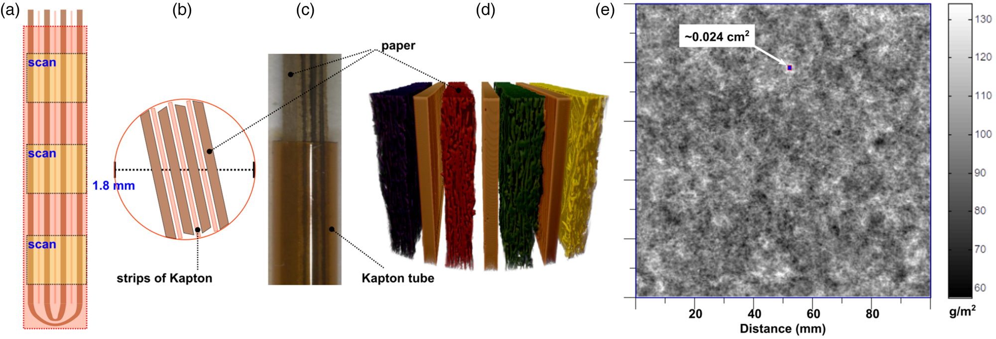
Fig. 1. Paper strips in a Kapton tube (a–d). Overview of the paper strip alignment within the tube (a,b). Optical image showing the paper and Kapton strips inserted in the tube (c). 3D visualization of binarized image data inside the Kapton tube (d).  $\beta$-radiograph of the uncompressed sample (e).
It is worth pointing out that this sample preparation also enables us to keep the registration of the scanned volume with respect to the paper sheet (Fig. 1e). This, in turn, allows us to (i) relate the orientation of the reconstructed 3D images to the machine and cross-direction and (ii) to deliberately pick and compare regions from the paper sheet.
We successfully employed this sample setup at two synchrotron radiation  $\mu$-CT facilities. The uncompressed paper samples were imaged in the absorption mode with an energy of $20$ keV, at the TOMCAT beamline (Stampanoni et al., Reference Stampanoni, Groso, Isenegger, Mikuljan, Chen, Meister, Lange, Betemps, Henein and Abela2007) of the Swiss Light Source at the Paul Scherrer Institute. For this purpose, a CMOS camera (pco.edge, $2560 \times 2160$ pixel) with a magnification of 10 was used. This leads to a field of view of $1.7 \times 1.4\, {\rm mm}^{2}$ and a final voxel size of 0.65 $\mu {\rm m}$, where 1501 projections were recorded over an angular range of $180^{\circ }$ with an exposure time of 250 ms. The tomographic reconstructions were performed by means of the Gridrec algorithm (Marone & Stampanoni, Reference Marone and Stampanoni2012). In total, 150 volumes were obtained in 27 scans that covered a totally scanned area of approximately 2.9 cm $^{2}$ (Fig. 1). Note that for those 27 scans, the measurements were performed with a different number of samples per scan. More precisely, 22 scans were obtained with six samples per scan, four scans with four samples, and two scans with one sample. The compressed samples were imaged in inline phase contrast mode at the P05 beamline of the PETRA III storage-ring at DESY in Hamburg (Haibel et al., Reference Haibel, Beckmann, Dose, Herzen, Ogurreck, Müller and Schreyer2010; Wilde et al., Reference Wilde, Ogurreck, Greving, Hammel, Beckmann, Hipp, Lottermoser, Khokhriakov, Lytaev, Dose, Burmester, Müller and Schreyer2016). The synchrotron beam was generated with an undulator and monochromatized with a double crystal monochromator to an energy of $20$ keV. After transmitting the sample, the monochromatic X-rays were transformed into visible light using a CdWO4 scintillator. The optical lens system in combination with a CMOS camera (KIT CMOS, $5120 \times 3840$ pixel) covered a field of view of $3.29 \times 2.46\, {\rm mm}^{2}$. The resulting pixel size of the system was $0.64\, \mu {\rm m}$, where 2400 projections were recorded over an angular range of $180^{\circ }$ with an exposure time of 60 ms. Furthermore, four samples were measured in each scan with a distance of 40 mm between the sample and the scintillator. For the tomographic reconstruction of the sample, the MATLAB-based (The MathWorks, USA) library Astra Toolbox (Van Aarle et al., Reference Van Aarle, Palenstijn, De Beenhouwer, Altantzis, Bals, Batenburg and Sijbers2015, Reference Van Aarle, Palenstijn, Cant, Janssens, Bleichrodt, Dabravolski, De Beenhouwer, Batenburg and Sijbers2016) was used. In total, we obtained 52 volumes in 13 scans. For these volumes, a two times binning was used to give a resulting voxel size of 1.3 $\mu {\rm m}$.
Figure 2 shows 2D slices of the grayscale images representing the microstructure of the considered uncompressed and compressed paper materials. Here, one can observe that the differently performed measurements lead to different types of contrast, which, in turn, require different methods for segmentation, i.e., for the classification of individual voxels as cellulose material or its complementary void space. While the contrast in the images showing the uncompressed paper sheets allows for a segmentation based on absorption contrast by means of indicator kriging (Oh & Lindquist, Reference Oh and Lindquist1999) as in Machado Charry et al. (Reference Machado Charry, Neumann, Lahti, Schennach, Schmidt and Zojer2018), this is not possible for the image data representing the compressed paper sheets. In the latter case, the absorption contrast between cellulose and void space is low. However, a clear phase contrast at the boundary of the cellulose allows for a segmentation using a random forest classifier within the FIJI Weka Segmentation plugin (Schindelin et al., Reference Schindelin, Arganda-Carreras, Frise, Kaynig, Longair, Pietzsch, Preibisch, Rueden, Saalfeld, Schmid, Tinevez, White, Hartenstein, Eliceiri, Tomancak and Cardona2012; Arganda-Carreras et al., Reference Arganda-Carreras, Kaynig, Rueden, Eliceiri, Schindelin, Cardona and Seung2017). For resolving the pore structure and the thickness, we determined top and bottom surfaces of the binarized volumes with the rolling ball approach (Sternberg, Reference Sternberg1983) that has already been used for 3D image data of paper materials (Svensson & Aronsson, Reference Svensson and Aronsson2003; Sintorn et al., Reference Sintorn, Svensson, Axelsson and Borgefors2005; Chinga-Carrasco et al., Reference Chinga-Carrasco, Axelsson, Eriksen and Svensson2008; Machado Charry et al., Reference Machado Charry, Neumann, Lahti, Schennach, Schmidt and Zojer2018) and battery electrodes (Kuchler et al., Reference Kuchler, Prifling, Schmidt, Markötter, Manke, Bernthaler, Knoblauch and Schmidt2018). For the present study, we re-binned the image data of the uncompressed sample such that the voxel sizes of both samples coincide. Doing so, we ensure that the results from statistical image analysis are comparable to each other.
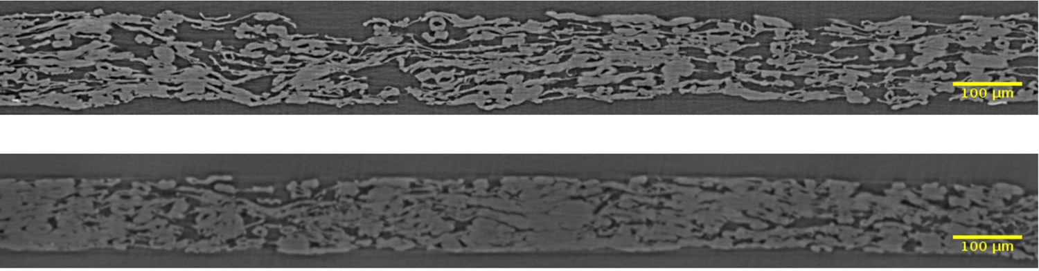
Fig. 2. Cross-sections of greyscale images obtained by  $\mu$-CT, which represent the microstructure of the uncompressed (top) and compressed (bottom) sample, respectively.
Statistical Image Analysis
Using methods of spatial statistics (Ohser & Schladitz, Reference Ohser and Schladitz2009; Chiu et al., Reference Chiu, Stoyan, Kendall and Mecke2013), we quantify local variations in the uncompressed and compressed paper sheets. For this purpose, we determine spatially resolved microstructure descriptors by partitioning all binarized data sets into non-overlapping cutouts. These cutouts, which serve as local inspection regions, are square-shaped in the lateral direction and contain the entire thickness of the paper sheet as described in Neumann et al. (Reference Neumann, Machado Charry, Zojer and Schmidt2021). The side length of the squares is varied between  $30$ and $330\, \mu {\rm m}$. In total, for statistical image analysis, we take 306 and 352 cutouts in the uncompressed and compressed case into account, respectively. This means that in both cases, we use an area of more than $30\, {\rm mm}^{2}$ for our analysis. As microstructure descriptors, we consider spatially resolved thicknesses, porosities, and mean geodesic tortuosities. Note that the mean geodesic tortuosity $\tau _{0}$ quantifies the length of shortest transportation paths through the pore space. More precisely, for a given cutout, we compute the mean value of the length of shortest transportation paths going from the inner surface of the paper sheet intersected with this cutout through the pore space to the outer surface of the sheet. Then, $\tau _{0}$ is defined as this mean value divided by the local thickness of the sheet. For further details regarding mean geodesic tortuosity, we refer to Stenzel et al. (Reference Stenzel, Pecho, Holzer, Neumann and Schmidt2016) and Neumann et al. (Reference Neumann, Hirsch, Staněk, Beneš and Schmidt2019). In general, for $r> 0$, the descriptor $\tau _{r}$ is analogously defined (Neumann et al., Reference Neumann, Machado Charry, Zojer and Schmidt2021), but only paths which can be passed by balls of radius $r$ (in $\mu {\rm m}$) are taken into account. In this study, we particularly consider $\tau _{0}$ and $\tau _{3.0}$. The statistical analysis of local microstructure descriptors provides the variability of local thicknesses, local porosities, and the local tortuosities $\tau _{0}$ and $\tau _{3.0}$ for paper sheets before and after compression. The pairwise interdependence between local porosities and both local tortuosities as well as local thicknesses is quantified by means of correlation coefficients.
Results
Changes in Macroscopic Properties
To begin with, we consider macroscopic properties of the samples before and after compression in order to quantify the compression-induced changes. The experimentally measured values are shown in Figure 3. This figure comprises the values of the basis weight, the caliper-based thickness, the Bekk smoothness parameter, and the Gurley retention time.
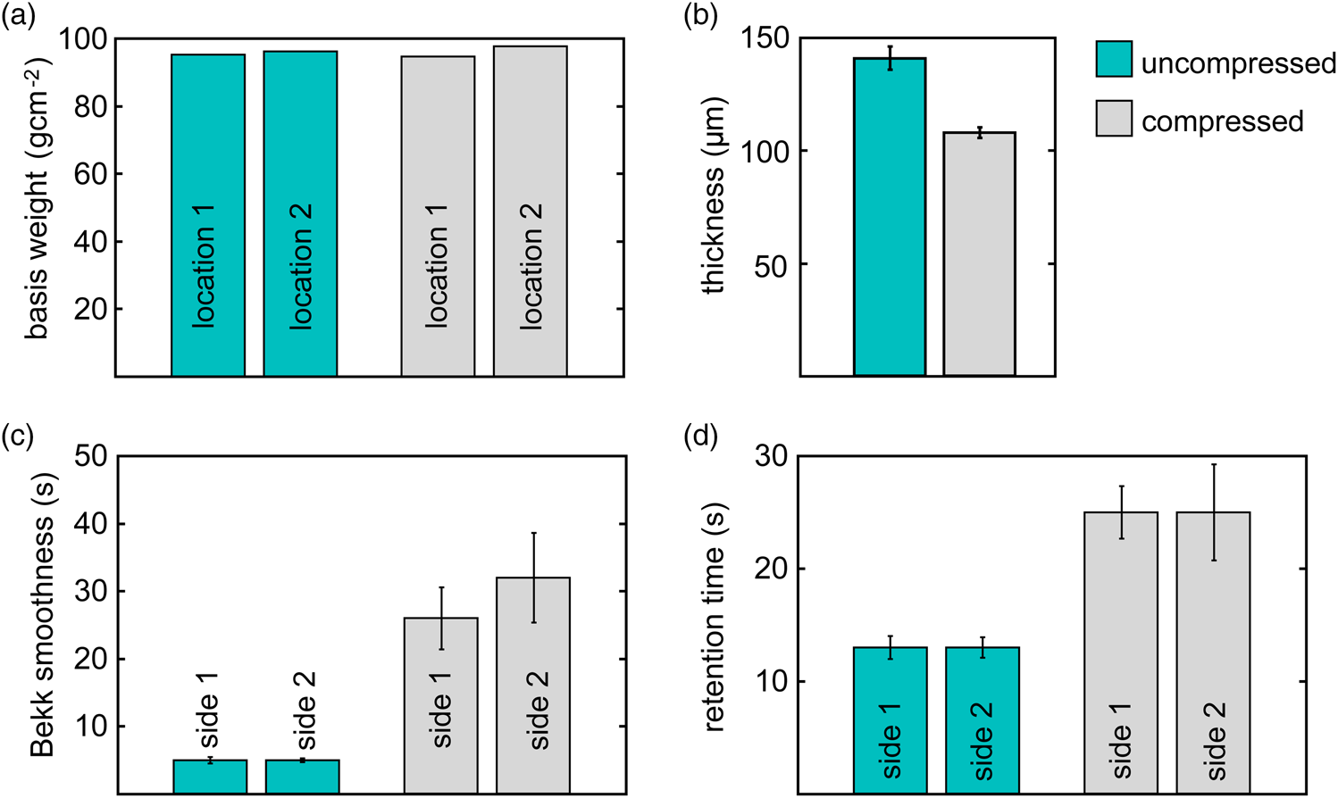
Fig. 3. Comparison of uncompressed (blue) and compressed paper (grey) in terms of (a) basis weights (measured at two different locations), (b) caliper-based thickness, (c) Bekk smoothness parameter, and (d) Gurley retention time. The Gurley retention time and the Bekk smoothness are measured with respect to the two boundary sides of the paper sheets (side 1 and side 2 which correspond to bottom and top surface), while the basis weights are measured at two different locations of the paper sheets. The error bars show the corresponding standard deviations.
The basis weight measured (at two different locations) for the samples before and after compression stays essentially the same at approximately 100 g/m $^{2}$, see Figure 3a. The variation of the basis weight was assessed by inspecting the power spectra of the $\beta$-radiographs (Norman & Wahren, Reference Norman and Wahren2020) with a size of $10\times 10$ cm $^{2}$. The radiograph of the uncompressed sample is exemplarily shown in Figure 1e; all further $\beta$-radiographs and the related power spectra are provided in Supplementary Material. The power spectra reveal a larger variation in the compressed sample across all length scales between 0.2 mm and 2 cm. Below 1.2 mm, i.e., on length scales observable within the field of view of $\mu$-CT scans, the variation is only subtly enhanced after calendering. This implies that calendering did not strictly preserve the local mass density, but did not profoundly alter the lateral fiber arrangement either.
The smoothness of surfaces is characterized using the Bekk method. The Bekk smoothness parameter informs on the time (in seconds) for a fixed volume of air to leak between the surfaces of a paper sample and a smooth glass. According to Figure 3c, the Bekk smoothness parameters associated with top and bottom surface strongly increase after calendering, which is in line with the intended purpose of calendering. Remarkably, the variation of the smoothness parameters increases with calendering as well. Formerly dominating air-leakage pathways permitting large volume fluxes are likely replaced by a large variety of leakage pathways carrying considerably less air volumes. The caliper-based thickness (Fig. 3b), i.e., the apparent thickness associated with the most protruding regions of the paper sheets, shows a marked reduction after compression from 141 to 108  $\mu {\rm m}$. Also, the measured variation of thickness reduces due to the surface smoothing.
The Gurley retention time shown in Figure 3d is inversely proportional to the volume flux of air that each of the two paper samples permits. Regardless whether air is transported from the top to bottom surface (side 1 in Fig. 3d) or vice versa (side 2 in Fig. 3d), compression leads to a twice as high retension time and a marked enhancement in variation. The corresponding decrease in volume flux indicates a substantial change in the pore space available for air transport.
Local Changes of the Microstructure
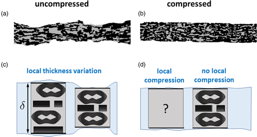
To relate this profound reduction in volume flux to local properties of the pore space, we turn to the inspection of the microstructure. Illustrative cutouts taken from the 3D microstructure of each of the two paper samples are shown in Figures 4a and 4b and emphasize the most striking differences between them. The uncompressed sample shows a marked corrugation of the surface that is, at least in part, caused by a spatially fluctuating number of vertically stacked fibers (black regions in Fig. 4a). Correspondingly, less fibers lead to a reduced local thickness  $\delta$ in that region, as illustrated in Figure 4c. In contrast, the compressed sample shows rather smooth surfaces and an apparently constant and overall reduced thickness. Beyond thickness reduction and smoothing, hard-nip calendering is expected to compact the paper transversely, such that the most protruding fiber-rich regions are compacted in the vertical direction. The less a feature protrudes beyond the final thickness, the less the paper is locally compacted. The microstructure of regions, in which fibers do even not protrude at all, are essentially preserved. In this way, calendering transforms regions of different thicknesses into regions of different degrees of compression and, thus, of different mass densities. Figure 4d illustrates that this compression acts locally. Depending on the location, the sample is compressed to a fraction of the original thickness of the sample. Some regions are not compressed at all and hence preserve their original thickness and structure. Turning back to the cross-section of the compressed sample shown in Figure 4b, we may indeed discern between regions with a high density of fibers (indicated in black) related to a marked compression and regions with a lower density of fibers, representing small if not even absent compression. To substantiate these observations, we perform statistical image analysis where the focus is on four selected, local microstructure descriptors which have been introduced above: thickness, porosity, mean geodesic tortuosity, $\tau _{0}$, related to all pathways, and mean geodesic tortuosity, $\tau _{3.0}$, associated with high-volume pathways exhibiting a minimum diameter of 3 $\mu {\rm m}$. This image analysis provides (i) the univariate distributions of these quantities, (ii) the pairwise interdependence between them, and (iii) their dependence on the number and size of the local inspection regions. While the former two quantitatively assess the impact of calendering, the latter will inform us, whether the data set has been representative for the paper sheet.

Fig. 4. Cross-sections of the binarized 3D images showing the microstructure before and after compression by hard-nip calendering (a,b). Fibers are represented in black, while the inner pores are represented in grey. The cutouts are 0.64 mm long. Schematic illustration of the local microstructure (c,d) showing local thickness variations before calendering (c) and locally varying degrees of compression after calendering (d). While thinner regions with the unaltered local structure may persist, regions with a larger local basis weight will be densified. For these densified regions, symbolized by the question mark, the compression-induced change of the microstructure is a priori unknown.
Figure 5 compares the univariate distributions of the selected local quantities in terms of the probability density functions for cutout sizes of  $90$ and $330\, \mu {\rm m}$. Each panel displays the distribution for the uncompressed sample in the upper half and the corresponding distribution for the compressed sample in the lower half. Note that we determined the probability density functions by diffusion-based kernel density estimation (Botev et al., Reference Botev, Grotowski and Kroese2010). A first inspection suggests that calendering induced profound changes in the local thickness, local porosity, and in $\tau _{3.0}$. To quantify the interdependence between the local microstructure descriptors, we determined the correlation coefficients between path length-related descriptors and local porosity as well as local thickness. This set of correlation coefficients, shown as functions of the cutout size in Figure 6, suggest a marked difference in the microstructures.
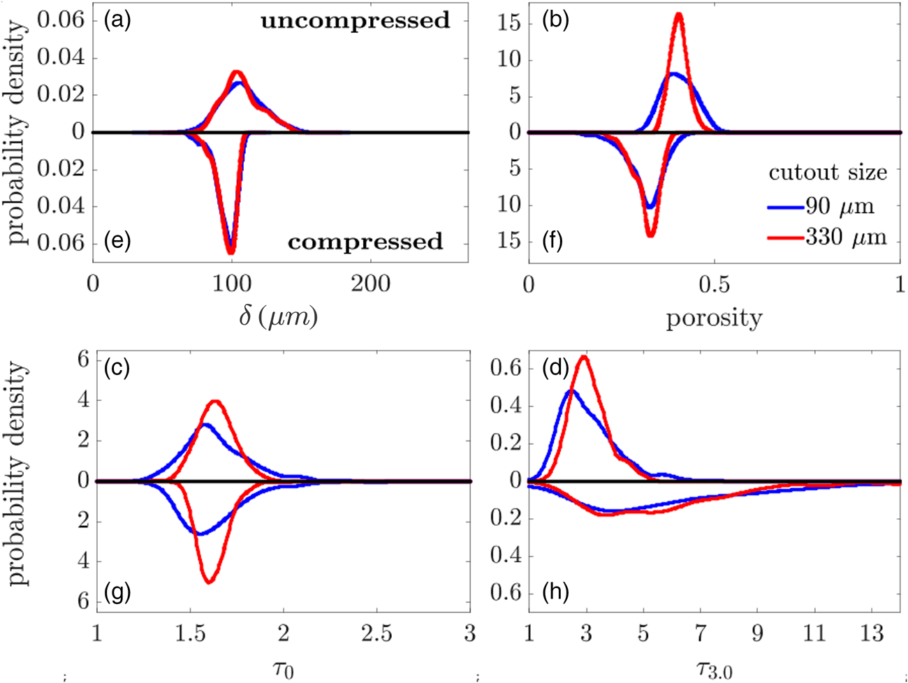
Fig. 5. Univariate distributions of four local descriptors before and after compression for cutout lengths of 90 $\mu {\rm m}$ and 330 $\mu {\rm m}$. In each panel, the probability densities in the upper panel refer to the uncompressed sample and the ones in the lower panels to the compressed sample. The descriptors considered here are local thickness (a,e), local porosity (b,f), and the local mean geodesic tortuosities $\tau _{0}$ (c,g) and $\tau _{3.0}$ (d,h).
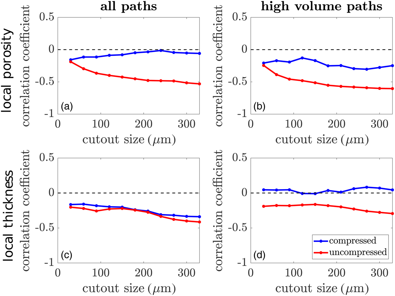
Fig. 6. Comparison of correlation coefficients between pairs of local microstructure descriptors before and after compression. Correlation coefficients between local porosity and  $\tau _{0}$ (a) respectively $\tau _{3.0}$ (b), as well as between local thickness and $\tau _{0}$ (c) respectively $\tau _{3.0}$ (d) are shown for various cutout sizes.
However, before inspecting the differences between the paper samples revealed by univariate distributions and correlation coefficients more closely (as will be done in the following section), it is important to evaluate first whether the estimated local distributions are representative for the samples. This is a crucial aspect, since, in case that the number of local inspection regions used for our statistical image analysis is too low, we may, e.g., miss regions of pronounced fiber aggregation or regions in which fibers are particularly loosely packed. Therefore, the obtained statistical results might be biased by the location of the inspection regions. We test the requirement of considering sufficiently many local inspection regions. For this purpose, the discrepancy between the distributions computed with all cutouts and the distributions computed with a subset of all cutouts, i.e., 306 cutouts for the uncompressed sample and 324 for the compressed sample, is determined. For this purpose, we consider a fixed cutout size of 330  $\mu {\rm m}$. The results are shown in Figure 7, where the discrepancy is measured in terms of the Kolmogorov distance. Note that the Kolmogorov distance between two probability distributions is defined as the supremum distance of the corresponding cumulative distribution functions. In Neumann et al. (Reference Neumann, Machado Charry, Zojer and Schmidt2021), we used the Kolmogorov–Smirnov test based on the Kolmogorov distance to validate a parametric model for the joint distribution of local porosity and local path length-related descriptors. Figure 7 shows that for all microstructure descriptors, a number of at least 200 cutouts has to be considered such that the Kolmogorov distance is below 0.05. Due to the increasing variability of local microstructure descriptors with decreasing cutout size, this statement remains valid for cutout sizes below $330\, \mu {\rm m}$. Moreover, we provide .mp4-files as Supplementary Material showing the evolution of the univariate distribution of each descriptor, when—step-by-step—more local inspection regions are incorporated until all available cutouts are used in the end. The corresponding file names are listed in Table 1.
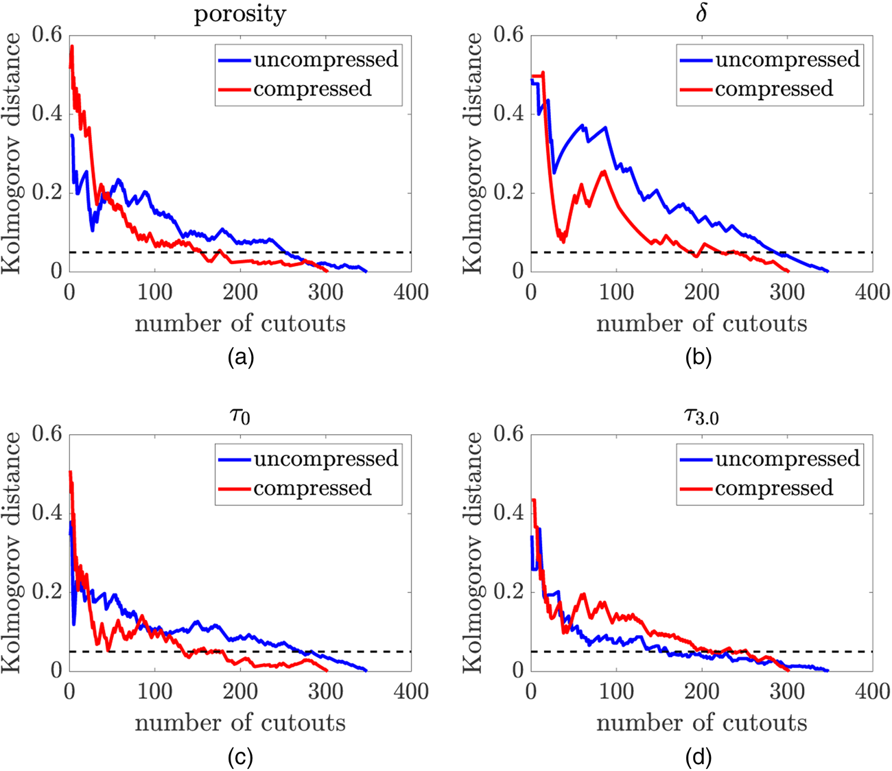
Fig. 7. Discrepancy between the distributions of the local microstructure descriptors porosity (a), thickness  $\delta$ (b), and the path length-related descriptors $\tau _0$ (c) and $\tau _{3.0}$ (d) computed with all cutouts and the corresponding distribution computed with a subset of cutouts. For this purpose, a fixed cutout size of $330\, \mu {\rm m}$ is considered. The $x$-axis indicates the number of cutouts taken into account and the discrepancy is quantified by means of the Kolmogorov distance for both the compressed and the uncompressed sample. The black dotted lines represent the level of Kolmogorov distance of 0.05.
Table 1. Filenames related to given geometrical descriptors in the uncompressed and compressed case.

Not only the number, but also the size of the cutouts is expected to have an impact on the univariate distributions of local microstructure descriptors. For example, Sampson (Reference Sampson2001) illustrated that the variance in local basis weight decreases with cutout size. For all four local descriptors, considered in the present article, the mean values in dependence of the cutout size are shown in Figure 8, where the  $0.95$- and $0.05$-quantiles are additionally given for quantifying the variability. The complete univariate distributions are provided in Supplementary Material.

Fig. 8. Mean values of local porosity (a), local thickness (b), local tortuosities  $\tau _{0}$ (c), and $\tau _{3.0}$ (d) over the considered cutout sizes. The areas between the $0.95{\text-}$ and $0.05{\text{-quantiles}}$ are shaded, i.e., for a given cutout size, $90\percnt$ of the corresponding local microstructure descriptors are contained in these shaded areas.
Discussion
Distributions of Local Microstructure Descriptors
The univariate distributions of local microstructure characteristics reveal profound differences between the two samples: the distributions of local thicknesses (Figs. 5a and 5e) and local porosities (Figs. 5b and 5f) fully corroborate the expected impact of calendering (Chinga et al., Reference Chinga, Solheim and Mörseburg2007; Vernhes et al., Reference Vernhes, Dubé and Bloch2010). The probability density function of the local thickness takes its maximum at approximately 110  $\mu {\rm m}$ for the uncompressed sample and at approximately 100 $\mu {\rm m}$ for the compressed sample, respectively. Beyond that, however, the probability density function of the compressed sample sharply decreases after the maximum value. In other words, the local thicknesses do not exceed 120 $\mu {\rm m}$ after compression. However, note that—interestingly—variations toward smaller values of the local thickness behave similar for the compressed and uncompressed case (cf. also Fig. 8b). This markedly changed variability of the local thickness is fully in line with the caliper-based thickness probing and with the visual inspection of the cutouts in Figures 4a and 4b. In terms of local porosity, compression causes a decrease of mean local porosity from 0.43 to 0.34. The slightly skewed distribution in Figure 5f suggests that the pores are not uniformly compressed. A glance on the pores found in the cutouts, shown as gray regions in Figures 4a and 4b, suggests that, in particular, large pores undergo a disproportionately large compression.
Beside porosity, also the length and thickness of pathways through the pores, i.e., the sinuosity and capacity of pathways, are expected to affect the volume flux of air and, hence, the Gurley retention time. We expect that calendering introduces changes in location, length, and thickness of local pathways, which affects the morphology of transportation paths as follows. First, in average, the paths—all paths as well as paths exhibiting a diameter of at least  $3\, \mu {\rm m}$—become longer. Second, the variability of the lengths of transportation paths is increased. Three major reasons lead to these assumptions: (i) the practically unchanged regions will pertain their local tortuosities; (ii) for the other regions, the following two complementary (limiting) cases suggest that the tortuosity ought to increase due to local compression. When, e.g., hypothetically assuming a uniform transversal compression of pore space and fibers alike, the length of established pathways can be shown to shrink less than (or equally as) the local paper thickness. Then, the mean geodesic tortuosity increases with increasing degree of compression. When, however, rather assuming an exclusive transversal compression of the pore space, i.e., assuming rigid fibers, the local porosity shrinks. In this case, additionally to the afore-mentioned mechanism, the topology of the pore space is not necessarily preserved either, e.g., because fibers getting in contact may block pathways. Then, the tortuosity rises due to the known negative correlation between porosity and tortuosity (Neumann et al., Reference Neumann, Machado Charry, Zojer and Schmidt2021). Our assumption regarding the increased local variations of the length of transportation paths is based on a third argument. Namely, (iii) as calendering introduces regions of different degrees of compression, compared the arguments (i) and (ii) mentioned above, the local variations in tortuosity and the overall mean geodesic tortuosity are expected to increase.
The distributions of  $\tau _{0}$ associated with all pathways (Figs. 5c and 5g) do not suggest marked changes under compression. Compression changes the sample-averaged value of $\tau _{0}$ merely from 1.64 to 1.63 and induces a bit more skewed distribution as well as a slightly reduced variance of $\tau _{0}$. In stark contrast to this, the descriptor $\tau _{3.0}$ related to high-volume pathways is strongly affected by compression (Figs. 5d and 5h). Compression leads to a profound increase of high-volume path lengths. The sample-average of $\tau _{3.0}$ increases almost by a factor of two from 3.08 to 5.94 for the largest cutout size of $330\, \mu {\rm m}$. The sample variance of the path lengths increases even more impressively, as path lengths exceeding the local thickness by more than a factor of ten non-negligibly contribute to the distribution of $\tau _{3.0}$. This implies that an overwhelming fraction of the pathways is oriented parallel to the paper surface. Considering a mean local paper thickness of approximately 100 $\mu {\rm m}$, there are pathways spanning lateral distances of more than 1 mm.
Pairwise Interdependence Between Local Descriptors
With the insights gained above, we now rationalize the similarities and differences regarding the pairwise interdependence between local microstructure descriptors, which were found for the uncompressed and compressed paper. At first, we focus on the correlation coefficients between path length-related descriptors and local porosity. Note that the correlation coefficients between local porosity and both path length-related descriptors,  $\tau _{0}$ and $\tau _{3.0},\;$ are negative (Figs. 6a and 6b) as expected in general for any porous material. With the growing size of the cutout, which is used as an inspection region, the correlation coefficient decreases for the uncompressed sample and stabilizes for large cutout sizes. This confirms the hypothesis conjectured based on maximum cutout sizes of $150\, \mu {\rm m}$ in Neumann et al. (Reference Neumann, Machado Charry, Zojer and Schmidt2021), where a detailed discussion about the influence of the cutout size on the interdependence between local porosity and local path length-related descriptors is provided, see Section 4 of Neumann et al. (Reference Neumann, Machado Charry, Zojer and Schmidt2021). The stronger variation of local microstructure descriptors induced by compression might be the reason that the correlation coefficients between local porosity and $\tau _{3.0}$ are still slightly fluctuating for large cutout sizes of the compressed sample (Fig. 6b). Remarkably, the absolute values of correlation coefficients decrease strongly after compression. This effect is stronger for $\tau _{0}$, where the correlation is nearly vanishing, compared to the results obtained for $\tau _{3.0}$. Recall that we observed only small changes in the univariate distribution of $\tau _{0}$, see Figure 5. In combination with the low correlation between local porosity and $\tau _{0},\;$ this suggests that—after compression—the topology of pathways remains nearly unchanged, while the porosity is reduced. This also explains that the negative correlation between local porosity and $\tau _{3.0}$ is stronger for the compressed compared to the uncompressed sample, since, by definition, more pores are required for the high-volume paths. The most critical condition to form such high-volume pathways is the ability to form an appropriately sized vertical connection between the fiber sheets (Sampson, Reference Sampson2003; Sampson & Urquhart, Reference Sampson and Urquhart2008). These findings suggest that the doubling of Gurley retention times upon calendering is caused, at least in part, by a marked reduction in porosity and by a reduction of transversal pore connections in high-volume pathways.
Moreover, we analyze the correlation coefficients between local thickness and path length-related descriptors. The results are shown in the lower panels of Figure 6, where one can observe a negative correlation between local thickness and path length-related descriptors. This means that—in average— $\tau _0$ and $\tau _{3.0}$ decrease with increasing thickness. An exception is $\tau _{3.0}$ in the compressed sample, where almost no correlation is observed. Before we discuss these results in detail, recall the results of Figure 5 showing that the local thickness variation is strongly reduced upon calendering. When considering all paths, i.e., the descriptor $\tau _{0},\;$ the correlation coefficients before and after compression are almost indiscernible (Fig. 6c). The reason for this might be a combination of two effects. First, as also suggested by the univariate distributions and by the correlation coefficients between local porosity and $\tau _{0}$, the topology of pathways remains unchanged after compression. Second, the impact induced by changes of local porosity is compensated by changes of the local thickness. Turning from $\tau _{0}$ to $\tau _{3.0},\;$ the negative correlation becomes slightly less pronounced before compression and vanishes after compression (Fig. 6d). Note that for the computation of path length-related descriptors of a given cutout, we consider those paths, the starting point of which is located within the cutout. However, the paths themselves might leave the cutout. Our results have shown that the high-volume paths (normalized by the local thickness) become longer after compression. This means that these paths will leave the cutout in which they start with high probability and thus the absolute values of the correlation coefficients between the local thickness and $\tau _{3.0}$ are negligibly small. We conjecture that the small deviations of the correlation coefficient around zero are artifacts of the estimation.
Influence of Local Inspection Regions
The discussion, provided above, shows that our statistical analysis allows us to unambiguously discriminate between the two paper samples. In this section, we address the influence of number and size of local inspection regions with an emphasis on the representativeness of data used in the present study. First, we show that the number of cutouts is chosen sufficiently large to reliably determine the univariate distributions of local descriptors. In a second step, we discuss the influence of the cutout size, i.e., the size of the local inspection regions, on these univariate distributions.
The results presented in Figure 7 as well as the evolution of univariate distributions, estimated from an increasing amount of data (Table 1), show that—regardless of the sample (before or after compression) and regardless of the considered local descriptor—at least 200 cutouts were necessary for a reliable estimation of the corresponding univariate distributions. We observe that the local thickness appears to be especially sensitive to the actual location of the cutouts the distribution is composed of. This observation underlines that our tomographic measurements probed indeed distinct regions. Moreover, we can conclude that for a reliable quantification of local variations based on statistical image analysis as performed in the present study, we require highly resolved image data representing an area of least  $200 \times ( 330\, \mu {\rm m}) ^{2} = 21.78\, {\rm mm}^{2}$. The close relationship between effective macroscopic properties and geometrical microstructure characteristics in general (Torquato, Reference Torquato2002) and path length-related descriptors in particular (Stenzel et al., Reference Stenzel, Pecho, Holzer, Neumann and Schmidt2016; Neumann et al., Reference Neumann, Stenzel, Willot, Holzer and Schmidt2020), let us strongly conjecture that the same size of image data is necessary to quantify local variations of macroscopic properties of the considered paper sheets, such as, e.g., their air permeance. Note that the necessary number of cutouts for a reliable determination of the univariate distributions of local microstructure descriptors itself depends on the underlying microstructure. This means that the given value of $21.78\, {\rm mm}^{2}$ cannot be considered as a universal constant for all paper materials.
The results with respect to the influence of the size of local inspection regions on the mean values and corresponding  $0.95$- and $0.05$-quantiles are presented in Figure 8. One can observe that the strongest decrease of the variability occurs when increasing the cutout size from $30$ to $90\, \mu {\rm m}$. But even if the domain of uncertainty between the considered quantiles becomes smaller with increasing cutout size, it remains relatively large for the cutout size of $330\, \mu {\rm m}$. Note that this variability of microstructure descriptors for cutout sizes of $330\, \mu {\rm m}$ does not contradict the results obtained in Rolland du Roscoat et al. (Reference Rolland du Roscoat, Decain, Thibault, Geindreau and Bloch2007), where REV sizes between $200 \times 200\, \mu {\rm m}$ and $330 \times 330\, \mu {\rm m}$ in the lateral direction are determined using methods developed in Kanit et al. (Reference Kanit, Forest, Galliet, Mounoury and Jeulin2003). As already mentioned in the Introduction, the microstructure characteristics computed from the REV in Rolland du Roscoat et al. (Reference Rolland du Roscoat, Decain, Thibault, Geindreau and Bloch2007) still exhibit a certain variability.
Conclusion
Our multilayer stack configuration allows us to feasibly and efficiently obtain large microstructure data sets of paper by  $\mu$-CT at a resolution that permits a detailed analysis of the pore space. Each scan provides multiple, virtual volumes at once. Inserting the paper stack into a Kapton tube prevents not only the use of any adhesives, but also allows us to readily scan other paper regions without changing the sample. The total area comprised by the individually scanned volumes reaches the order of square centimeters.
Applying the proposed multi-layer stack configuration to paper material before and after calendering allows us for a data-driven investigation of the sample size, which is necessary to reliably extract the distribution of local microstructure descriptors. We consider local porosity, local thickness, and local path length-related descriptors. Our main conclusion is that, for reliably quantifying local variations of the paper materials considered in the present study, an area in the order of  $20\, {\rm mm}^{2}$ is required. This supports the results of Kritzinger et al. (Reference Kritzinger, Hirn, Donoser and Bauer2008), who have shown that—even if regions at different locations are considered—an area of several square millimeters is required to reliably determine the distribution of local thickness for coated paper sheets. Moreover, our results are in line with Dirrenberger et al. (Reference Dirrenberger, Forest and Jeulin2014), who have demonstrated that the analysis of fiber-based materials generally requires gigantic REVs.
Beside the issue of representativity, our study reveals quantitative insights regarding the influence of calendering on local microstructure descriptors. In particular, high-volume pathways, being predominantly responsible for the volume flux of air, are strongly affected by compression. An overwhelming fraction of each of these pathways is oriented parallel to the paper surfaces. Compression suppresses the forming of appropriately sized transversal openings between the fiber sheets such that pathways must cover much larger distances prior finding a suitable transversal connection.
Supplementary material
To view supplementary material for this article, please visit https://doi.org/10.1017/S1431927621012563.
Acknowledgments
The authors gratefully acknowledge financial support from the Christian Doppler Research Association, Federal Ministry for Digital and Economic Affairs, and the National Foundation for Research, Technology, and Development, Austria.


 Open access