
From Weinreich, Labov, and Herzog (Reference Weinreich, Labov, Herzog, Lehmann and Malkiel1968:188) onward, it has often been observed that the grammar of a speech community is more regular than the grammar of individuals (cf. e.g., Ashby, Reference Ashby2001:13). It appears that the same is true of patterns of language change, based on more recent studies of individual speaker behavior in real time. That is, the overall trajectory of change of a linguistic variant in a speech community appears to be more regular than the trajectories of change for individual speakers in the community. Again, from at least Weinreich et al. (Reference Weinreich, Labov, Herzog, Lehmann and Malkiel1968:113) onward, it has been observed that the trajectory of community change is an S-curve: “the overall changes … display an S-shaped curve despite the variation in the behavior of individual words, speakers, texts, geographical regions, or social classes over the trajectory of the change” (Blythe & Croft, Reference Blythe and Croft2012:281). But individual speaker trajectories are quite different, even if the cumulative outcome for the community is an S-curve.
We examine certain types of variation in the behavior of individual speakers and its relationship to community change and present a mathematical model that accounts for the patterns, based on the model presented in Baxter, Blythe, Croft, and McKane (Reference Baxter, Blythe, Croft and McKane2006, Reference Baxter, Blythe, Croft and McKane2009; see also Blythe & Croft, Reference Blythe and Croft2012). The observed variation in individual trajectories is not as regular as the recurrent S-curve of community change. However, there are certain patterns related to an individual's lifespan from childhood to maturity that appear to be relatively robust (e.g., Bailey, Reference Bailey, Chambers, Trudgill and Schilling-Estes2002; Bailey, Wikle, Tillery, & Sand, Reference Bailey, Wikle, Tillery and Sand1991; Labov, Reference Labov1994; Nevalainen, Raumolin-Brunberg & Mannila, Reference Nevalainen, Raumolin-Brunberg and Mannila2011; Sankoff & Blondeau, Reference Sankoff and Blondeau2007; Tagliamonte & D'Arcy, Reference Tagliamonte and D'Arcy2009). Our model suggests explanations for certain patterns of language change across the lifespan and their relationship to community change.
We model patterns of individual speakers as they age, that is, language change across the lifespan (Sankoff & Blondeau, Reference Sankoff and Blondeau2007), focusing our attention on three patterns that have been reliably observed and certain explanations offered for those patterns. One explanation is essentially individual: changes in a speaker's flexibility in their linguistic behavior as they age. The other explanations are essentially interactional: who a speaker interacts with, how much she accommodates to the linguistic behavior of her interlocutors, and how she weights different variants of a sociolinguistic variable.
We model three patterns. The first is the apparent time construct, widely used to extrapolate real time changes from a sample of behavior of speakers of different ages collected at a single time (Bailey, Reference Bailey, Chambers, Trudgill and Schilling-Estes2002; Labov, Reference Labov1963; inter alia). The apparent time construct is based on a particular assumption about individual trajectories in a language change, namely that an individual speaker changes her linguistic behavior reflecting a community change through adolescence, but then more or less ceases to change her behavior afterward. To the extent that this observation is correct, it is attributed to a physiological/cognitive reduction of linguistic flexibility postadolescence. In fact, it has been documented that adult speakers also may adjust their linguistic behavior with respect to an ongoing community change, although on the whole the apparent time construct remains a reasonably accurate gauge of an ongoing change (Bailey, Reference Bailey, Chambers, Trudgill and Schilling-Estes2002:329–330; Wagner, Reference Wagner2012a:377).
The second pattern is the adolescent peak (Cedergren, Reference Cedergren and Lowenberg1988; Labov, Reference Labov2001:446–465; Tagliamonte & D'Arcy, Reference Tagliamonte and D'Arcy2009). The adolescent peak is an anomaly in the otherwise S-curved trajectory of community change found in apparent time studies. It is assumed to result from an individual trajectory of change reflecting the child's primary exposure to different speakers at different stages of childhood (first caregivers, later older peers).
The third pattern is one that has been only recently remarked upon. There appear to be two contrasting ways in which adults adjust their linguistic behavior with respect to an ongoing community change (Nevalainen et al., Reference Nevalainen, Raumolin-Brunberg and Mannila2011; Sankoff & Blondeau, Reference Sankoff and Blondeau2007:580). The first is by gradual change in variable use of the incoming and outgoing variants over time. The second is more categorical behavior on the part of individual speakers, with individual speaker change happening rapidly (if a speaker changes at all). We argue that these two ways in which change over the lifespan takes place reflect in part differences in the degree to which speakers accommodate to their interlocutors in the speech community.
MODELING LANGUAGE CHANGE IN THE SPEECH COMMUNITY
Human society and social behavior, including language, is a good example of a complex adaptive system. A complex adaptive system can be characterized by the following traits (Beckner, Blythe, Bybee, Christiansen, Croft, Ellis, Holland, Ke, Larsen-Freeman, & Schoenemann, Reference Beckner, Blythe, Bybee, Christiansen, Croft, Ellis, Holland, Ke, Larsen-Freeman and Schoenemann2009:1–2). The system consists of multiple entities—speakers, in the case of language—interacting with one another. The behavior of the entities (speakers) evolves adaptively on the basis of past and present interactions, and future behavior is determined by past and present interactions. The system is complex in that a range of competing factors influence the behavior of the interacting individuals and hence the system as a whole. In the case of language, a wide range of physiological, cognitive, and social factors interact to produce the behavior of individual speakers and hence of the speech community as a whole.
The variationist approach to language change treats language as a complex adaptive system. Speakers interact with each other in a speech community. Their linguistic behavior is “outward bound” (Labov, Reference Labov2012:265, 267): it responds to the linguistic patterns experienced in their speech community. As a result, a speaker's linguistic behavior is variable, affected by the interaction of many different factors, social, language-internal, and otherwise. A speaker's language behavior changes over time in response to the patterns of variation of linguistic behavior to which she is exposed. In this respect, the variationist approach to language change is an example of a usage-based model (Bybee, Reference Bybee2001, Reference Bybee2007, Reference Bybee2010), in which speaker knowledge about her language is variable and responds to interactions with other speakers (that is, language use). Language change at the community level results from the cumulative effect of language behavior at the level of linguistic and social interactions among individuals.
The mathematical model proposed by Baxter et al. (Reference Baxter, Blythe, Croft and McKane2006, Reference Baxter, Blythe, Croft and McKane2009) is based on an evolutionary model of language change proposed by Croft (Reference Croft2000) that integrates usage-based and variationist approaches to language change. The central hypothesis of the model is that language change emerges from the replication of linguistic structures in utterances produced by speakers. Language use is inherently variable: replication generates variation in both phonological and morphosyntactic structure. Language change in a speech community is the cumulative effect of the evolution of the tokens of linguistic structures (called “linguemes” by Croft) as they are replicated by speakers as they interact with each other over time. Croft's model shares features with other complex adaptive system models of language change, such as Wedel's (Reference Wedel2007) model of the acquisition of phonological regularity and Stanford and Kenny's (Reference Stanford and Kenny2013) model of vowel chain shifts. All of these models include acquisition through interactions with other speakers; knowledge about language variation including representation of exemplars of language use by the speaker; and feedback from interactions, leading to changes in speaker knowledge about their language over time.
Four mechanisms of language change
Baxter et al. (Reference Baxter, Blythe, Croft and McKane2009:269–272; see also Blythe & Croft, Reference Blythe and Croft2012:272–277) derived four mechanisms of language change from their model of speaker interaction and language change. They called these mechanisms replicator selection, neutral interactor selection, weighted interactor selection, and neutral evolution. Replicator selection and neutral evolution are found in population genetics, but the two types of interactor selection are specific to models of cultural evolution with human agents producing cultural artifacts such as linguistic forms.
The mechanism that corresponds to fitness in population genetics models is called replicator selection by Baxter et al. (Reference Baxter, Blythe, Croft and McKane2009:269–270). Differential, that is, asymmetric weighting of variant replicators by speakers, leads to differential replication of the replicators, so that one replicator (variant) is propagated and the other falls out of use. Although the model (or the mathematics) does not say anything about what brings about the differential weighting of linguistic variants, we hypothesize that it represents differential social valuation of variants by speakers. This mechanism is associated with the classic Labovian sociohistorical model, though Labov himself noted that it was proposed by linguists before him (Labov, Reference Labov2001:24).
In addition to replicator selection, there are also two mechanisms for selection based on properties of the interactor, not the replicator: neutral interactor selection and weighted interactor selection. Neutral interactor selection occurs when differential replication of a linguistic variant by a speaker may occur as a consequence of different rates of interaction with other speakers, even if the variants produced by them are equally weighted (that is, no replicator selection is operating; Baxter et al., Reference Baxter, Blythe, Croft and McKane2009:270–271). Another way of describing this mechanism is that how I speak depends on who I talk to and how often I talk to them. Neutral interactor selection models social network structure, an important factor in many theories of language change (e.g., Milroy [Reference Milroy1987], although she incorporates replicator selection into her theory as well). Neutral interactor selection is symmetric: since it is simply how often a pair of speakers interact with each other, its effect is the same on both speakers.
Weighted interactor selection, on the other hand, is an asymmetric mechanism of interactor selection, in which a speaker accommodates (Giles, Reference Giles1973; Giles & Smith, Reference Giles, Smith, Giles and St Clair1979) more to her interlocutor in her linguistic behavior than the other way around (Baxter et al., Reference Baxter, Blythe, Croft and McKane2009:271). More generally, a speaker may accommodate more to one interlocutor than another, even if she interacts equally often with both of them. Weighted interactor selection is a plausible model of the leader-follower or adopter theories of diffusion of innovations (Rogers, Reference Rogers1995), which have also been proposed to play a role in language change (e.g., Labov, Reference Labov2001:356–360, Milroy & Milroy, Reference Milroy and Milroy1985; Nevalainen et al., Reference Nevalainen, Raumolin-Brunberg and Mannila2011; Sankoff & Blondeau, Reference Sankoff and Blondeau2007).
Finally, change can happen in finite populations of replicators by the stochastic nature of the replication process (whereby variants are produced). Rates of variants can fluctuate, and if this fluctuation goes to 100%, then the variant has replaced its competing variant. This process is called neutral evolution or genetic drift in population genetics; we call it “neutral evolution” to avoid confusion with linguistic drift (Sapir, Reference Sapir1921), which is an entirely different concept (cf. Baxter et al., Reference Baxter, Blythe, Croft and McKane2009:270). One important feature of neutral evolution is its sensitivity to the frequency of the variants: a more frequent variant is more likely to become fixed in the population than a less frequent variant. As a consequence, neutral evolution is a plausible model of the frequency effects documented in usage-based approaches to language behavior (e.g., Bybee, Reference Bybee2001, Reference Bybee2007, Reference Bybee2010).
A model of speaker interaction and change
Baxter et al. (Reference Baxter, Blythe, Croft and McKane2009) and Blythe and Croft (Reference Blythe and Croft2012) use a model incorporating these different mechanisms to examine theories of new-dialect formation and the S-curve trajectory of community change, respectively; the description of the model that follows is a summary of Baxter et al. (Reference Baxter, Blythe, Croft and McKane2009:272–277). The Baxter et al. model assumes that linguemes are independent, that is, it does not model interactions between linguemes such as chain-shifts (in contrast to Stanford & Kenny [Reference Stanford and Kenny2013]). Linguemes occur in variants; that is, a lingueme is a sociolinguistic variable. The speech community is made up of N speakers. Each speaker's knowledge about her language (her grammar) includes the frequency of use of each variant.
Speakers interact with (that is, talk to) one another and replicate variants in the process. The likelihood of interaction of speakers is given by a matrix G ij for speaker i interacting with interlocutor j; this matrix represents the social network structure of the speech community, and hence neutral interactor selection. (Stanford & Kenny [Reference Stanford and Kenny2013:125–127] also model network structure, but indirectly via a spatial grid in which speakers move around and interact with colocated speakers.) Speakers replicate (that is, produce) a lingueme a certain number of times in the interaction, and the variant(s) of the lingueme that they replicate is the result of a probabilistic function of the representation of the frequency of the variants in the speaker's mental grammar. Differential weighting of the variants, that is, replicator selection, plays a role in the speaker's selection of which variant to replicate. In the simplest case, one variant is selected by all speakers with an increased probability, which is controlled by a parameter that we will call b.
After the interaction, the speakers' grammars are updated; this corresponds to the feedback effect in the complex adaptive system. The updating process involves two variables. The first variable λ represents the weight assigned to the heard variants relative to the current grammar. That is, λ represents a speaker's receptiveness to changing her grammar; it corresponds to how flexible a speaker is in adjusting her linguistic behavior to the language she hears around her. As a small fraction λ of the grammar is replaced after each interaction, the influence of previously heard tokens is reduced. We can therefore also think of λ as controlling how long tokens are remembered. The amount of the grammar occupied by a token decays as exp(-λn), where n is the number of subsequent interactions that the speaker takes part in.
The second variable governing the updating of the speakers' grammars is the weight that a speaker assigns to her interlocutor's utterances compared to her own. The weight assigned by speaker i to interlocutor j's utterances is described by the matrix H ij. This matrix represents the degree of accommodation that the speaker makes to her interlocutor and hence weighted interactor selection. The speaker's grammar is thus updated until the next interaction.
Baxter et al. (Reference Baxter, Blythe, Croft and McKane2009) use this model to evaluate Trudgill's (Reference Trudgill2004) theory of new-dialect formation. Trudgill's theory advances two hypotheses about new-dialect formation as a result of the coming together of speakers from different source dialects (in this case, different parts of the United Kingdom) in a new speech community. The first is a “majority wins” rule: the variant that is the most frequent is the one most likely to be propagated in the new dialect (Trudgill, Reference Trudgill2004:113–115). The second is that no differential social valuation of variants or of speakers plays a role in the process of new-dialect formation. In terms of Baxter et al.'s (Reference Baxter, Blythe, Croft and McKane2009:271–272) mechanisms, Trudgill's theory argues that only neutral evolution and neutral interactor selection operate in new-dialect formation.
Baxter et al. (Reference Baxter, Blythe, Croft and McKane2009) tested Trudgill's theory using their model and data from the Origins of New Zealand project. The model confirms Trudgill's first hypothesis, that the majority variant is most likely to be propagated in new-dialect formation without any other social factors influencing propagation. As we have noted, one trait of neutral evolution is that the most frequent variant in the population is most likely to propagate. However, neutral evolution and neutral interactor selection alone (Trudgill's second hypothesis) are highly unlikely to lead to the fixation of the New Zealand English dialect in the time interval that the New Zealand English dialect actually formed, given other (empirically determined, but generous) values of relevant variables in the model. One reason for this is that the time for neutral interactor selection increases linearly with the population size.
Blythe and Croft (Reference Blythe and Croft2012) used the same model to examine the temporal trajectory, rather than the time scale, of community language change. When one variant successfully competes against another variant in being propagated across a speech community, the trajectory of the change is an S-curve (the full length of the S-curve may not be documented, and changes may cease before they have gone to completion; Blythe & Croft [Reference Blythe and Croft2012:278–281]).
Labov (Reference Labov2001:450) presented an equation yielding an S-curve for community change:
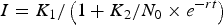 $$I = {K_1}/\left( {1{\rm} + {K_2}/{N_0} \times {e^{ - rt}}} \right)$$
where K 1 = maximum possible change in one year, K 2 = limits of the sound change, N 0 = initial year, r = rate of change, t = time (in years). This equation uses variables representing only community-level values: rate of change in the community and two variables related to the population using (or tokens of) the new variant, one being an arbitrary limit per year of change in population/token frequency for the new variant and the other set at 100%. In contrast, in Baxter et al.'s (Reference Baxter, Blythe, Croft and McKane2009) model, community-level change properties are an emergent property of individual speaker interactions and individual speaker social weighting of variants and interlocutors. Since we are interested in both individual language behavior across the lifespan and its trace in community change, Baxter et al.'s (Reference Baxter, Blythe, Croft and McKane2009) model is more suitable for our analysis.
Blythe and Croft (Reference Blythe and Croft2012) argued that the only selection mechanism that consistently produces an S-curve trajectory is replicator selection, that is, differential weighting of the linguistic variants themselves. Neutral evolution and neutral interactor selection (social network structure) produce highly fluctuating trajectories. Weighted interactor selection normally produces strong fluctuations; it can produce an S-like trajectory, but only under very specific assumptions representing social structures that are not characteristic of known speech communities (Blythe & Croft, Reference Blythe and Croft2012:287–291). Finally, the time length for replicator selection does not have the same sensitivity to population size that interactor selection does. Blythe and Croft's result implies that whatever else is going on in the propagation of a competing variant in a speech community, it must include differential weighting of the variants in order to produce the ubiquitous S-curves that are repeatedly observed.
In this article, we focus on the relationship between community change, that is, the population-level pattern of language change (the S-curve), and individual change. In particular, we examine hypotheses regarding the role of receptiveness (λ) in the apparent time effect and the role of social network structure (G ij) in the adolescent peak. We find that receptiveness does lead to the apparent time effect, but the adolescent peak is much less sensitive to social network structure than has been proposed. Finally, we examine individual paths of change and find that they result from the interaction of the rate of change (controlled by b) and degree of accommodation by a speaker to her interlocutors (H ij).
THE APPARENT TIME CONSTRUCT
Evidence and explanations for the apparent time construct
The apparent time construct has long been used to allow sociolinguists to make inferences about language change in progress from a single synchronic sample of speaker behavior. If there is a difference in linguistic behavior across speakers of different ages, then it is possible to infer that there is an ongoing change, with older speakers representing the earlier stage of the language and younger speakers representing the later stage. Although speakers are quite adaptive in their linguistic behavior up through adolescence, after adolescence flexibility in linguistic behavior drops off significantly, although adolescent and adult change can still occur (see Clark [Reference Clark2003:391–399] for a survey from an acquisition perspective, and Bailey [Reference Bailey, Chambers, Trudgill and Schilling-Estes2002] for a survey from a sociolinguistic perspective); we will examine patterns of postadolescent individual speaker change in this section. Hence a speaker's adult linguistic behavior, even decades later, reflects her linguistic behavior, and the linguistic behavior of the speech community, at the time of her adolescence or early adulthood.
The relationship between community change and individual change across the lifespan, particularly postadolescence, is addressed more directly by studies in which the linguistic behavior of a sample of speakers from a community are analyzed by age cohort (i.e., the input to an apparent time analysis) and across at least two different time points (i.e., a study in real time). These studies fall into two types: a panel study, in which the same speakers are tracked down and interviewed at a later time (or times); or a trend study, in which a new set of speakers is sampled at a later time, with a similar social profile to the set of speakers sampled at the first time.
Table 1 summarizes the results of several surveys of linguistic variables in apparent and real time. The studies summarized in Table 1 also sample speakers across the full lifespan, including middle age and old age. In these studies, data is presented that allow us to compare the behavior of the same age cohorts (or in the case of some panel studies, the same individuals) across at least two different time intervals (in many of the studies, the authors do not make this direct comparison). In one larger-scale panel study (Nahkola & Saanilahti, Reference Nahkola and Saanilahti2004), the panel data are given in aggregate, rather than by individual.
Table 1. Changes in adult individual linguistic behavior during a community change

Study: TR trend study; PA panel study, data aggregated by age cohort; PI panel study, individual data; n numerical data, % percentage data, gr graphed data only, f change in format frequencies (continuous variable).
Ages: number of age cohorts whose behavior is reported across at least two different times (TR, PA); or number of individuals whose data is reported across at least two different times (PI).
Times: number of different time samples.
In interpreting Table 1, one issue is that most studies do not indicate whether differences in speaker behavior from one time point to the next are significant (in fact, almost all studies give only percentage data). As a consequence, in presenting the results of our survey of studies of apparent and real time, we use a difference in linguistic behavior of 10% (that is, a speaker changes her use of a variant from X% to X + 10% or more) as significant, following in part the significance results in Sankoff and Blondeau (Reference Sankoff and Blondeau2007).Footnote 1
In more than half of reported cases of individual changes of variants undergoing community change, adults do not change their behavior by more than 10% after adolescence. Although Trudgill (Reference Trudgill1988:37) did not give numerical or percentage data for his restudy of Norwich, he stated that changes in adult linguistic behavior are “in most cases rather small,” and adults did not participate in more recent changes diffusing through the Norwich speech community. These observations imply that on the whole, the apparent time construct is supported (Bailey, Reference Bailey, Chambers, Trudgill and Schilling-Estes2002:324; Bailey et al., Reference Bailey, Wikle, Tillery and Sand1991; Wagner, Reference Wagner2012a:377). When adults are advancing, three patterns appear: all adults are advancing by a similar degree; older adults are advancing by a lesser degree than younger adults; and there are even cases of adults retreating from a community change. There are no reported instances to our knowledge of older adults advancing to a greater degree than younger adults in a community change. Finally, there is a more complex pattern revealed by the panel study of Montréal French /r/ that will be discussed and modeled later.
Modeling apparent time
To recapitulate, Baxter et al.'s (Reference Baxter, Blythe, Croft and McKane2006, Reference Baxter, Blythe, Croft and McKane2009) model starts with a community of N interlocutors; a pair of interlocutors are chosen to interact based on social network structure G ij; the effects of the interaction depend on the receptiveness λ of the interlocutor to change their behavior, the differential weighting b of the competing variants—necessary to produce the S-curve of language change—and to the differential weighting H ij given to their interlocutor's productions; the model evolves over a large number of interactions. To model apparent time, we modified Baxter et al.'s (Reference Baxter, Blythe, Croft and McKane2006, Reference Baxter, Blythe, Croft and McKane2009) model to allow the parameter λ, which controls receptiveness, to change over a speaker's lifetime and to allow speakers to die and be replaced by new speakers.
For the apparent time construct to be possible, this change should happen in such a way that a speaker's ability to change is greatest in childhood and adolescence and is considerably reduced in adulthood. For simplicity, the way that λ changes as a function of a speaker's age was made the same for every speaker. Because speakers in the population have a variety of ages at any given time, a range of λ values are present in the population. As we have already discussed, in real populations, some speakers change more than others, even among those having the same age. However, this approximation is sufficient to capture the aggregate behavior across the whole population.
There are many possible choices for this λ function. We chose to model the receptiveness λ as a function that decays smoothly with age. In this way, we do not artificially impose a change in cognitive behavior or abilities of speakers at a specific age. We seek a function that decays sufficiently quickly that speakers' linguistic malleability becomes significantly reduced after a certain age (though not necessarily completely eliminated), but slowly enough that speakers remain adaptable into late adolescence. One suitable function is an exponentially decaying function (see (2)), where a is the age of the speaker concerned, and β controls the speed of the decay.
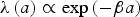 $$\lambda \left( a \right) \propto {\rm exp}\left( { - \beta a} \right)$$
To choose a sensible value of the parameter β, we simulated a speaker of a certain age, who initially uses a conventional variant almost exclusively, and who applies a replicator selection boost b to a second variant, while also interacting with a large population who exclusively use the new variant. The algorithm proceeds as in the main model, except that the single speaker only hears the new variant from her interlocutors. These conditions allow us to estimate the maximum change a speaker of a given change is able to make in their remaining lifetime. An example is shown in Figure 1a. A speaker below a certain threshold age is able to reach categorical usage of the new variant. Older speakers, on the other hand, initially move toward the new variant, but are not able to complete the change. We repeated the experiment for three values of the replicator selection strength, b, covering a broad range of feasible values (.001, .01, and .02). For each value of b, we also tried a broad range of rates of speaker interaction, 100 times per year, 10,000 times per year, and the more likely rate of 1000 interactions per year. Despite the large variation in parameter settings, we see that in all cases speakers older than about 25 years hardly change. The threshold age depends strongly on the parameter β and weakly on the strength b of the replicator selection, and on other details such as how many interactions a speaker participates in per year. The results for this decay function depend only weakly on the parameter H (a value of .02 was used in the results shown). We chose the parameter β = .4, as this gives fall-off at approximately 15 to 20 years of age, using reasonable values for the other parameters.
Figure 1. Final grammar value reached as a function of initial age, for a speaker of one variant immersed in a population of the new variant. (a) Speaker's λ value decays exponentially with parameter β = .4. Curves for three different replicator selection strengths, b = .001, .01, .02, (blue, red, and green, respectively) are shown. (b) Speaker's λ value decays as a power law with parameter γ = 2.0. Curves for the same three replicator selection strengths, b = .001, .01, .02, (blue, red, and green, respectively) are shown. In both plots, speaker uses the given lingueme in 1000 interactions per year (solid lines), producing 10 tokens in each interaction. Curves for 100 interactions per year (dotted) and 10,000 per year (dashed) are also shown. Initial usage of 1% is marked by the gray line. (Note: Color images can be viewed online at http://cambridge.journals.org/LVC.)
The disadvantage of using function (2) is that the fall-off may be too dramatic: speakers are able to change only a very little during adulthood. We can instead consider a power law decay function (3).
 $$\lambda \left( a \right) \propto {a^{ - \gamma}} $$
Choosing γ = 2 for this function again gives a fall-off in speaker response at around 15 to 25 years of age (though the precise age is more dependent on the replicator selection parameter b). Now, however, adult speakers remain able to continue to change, albeit much more slowly as shown in Figure 1b. Even adult speakers are able to change their usage by a few percentage points. Unlike the exponential decay, the amount of change adults are able to make depends on the accommodation parameter H. In the example shown, we used a moderate value of H = .02. Larger values would allow adults to change even more. As we will see, using either function (2) or function (3) gives qualitatively similar results, indicating that the exact choice of the decay function does not unduly influence our results.
For the main model, the full population is fixed at a certain size N. In the presence of replicator selection, the behavior of the model does not depend on population size, except for statistical fluctuations, which are larger for small populations. For the simulations described in the remainder of the article, we used a population size of N = 1000. This is large enough to give good statistics, representative of large populations, but not so large that model simulations become unduly onerous. Periodically one speaker is chosen to be removed and is replaced by a new speaker. (New speakers are given an age of 1, corresponding to roughly the age at which they may begin participating in the speech community.) The probability that a speaker of age a will be removed is given by an exponentially increasing hazard function exp(ωa) (Gompertz, Reference Gompertz1825). With ω = .085 this function results in a good approximation of the age distribution found in the United States, as evidenced by the 2009 mortality statistics (Arias, Reference Arias2014); see Figure 2. The mean longevity is 80 years. When a new speaker is created, she is essentially a “blank slate,” without any predefined grammatical knowledge. In her first conversation, she will take whatever tokens she hears from her interlocutor to set her initial grammar value. Subsequently she will interact as normal, adapting to her own utterances and those of their interlocutors. Apart from the first interaction speakers produce tokens probabilistically based on their current grammatical knowledge, as we have described. For this initial investigation, we chose the simplest network of social interactions possible: every speaker is equally likely to speak to every other, that is, the nondiagonal entries in the matrix G ij are all equal. Similarly, the accommodation weights H ij were also set to equal the same value H. In order to choose an appropriate order-of-magnitude estimate for the frequency of interaction, we refer to estimates made in Baxter et al. (Reference Baxter, Blythe, Croft and McKane2009:282) that a speaker may hear a million or more tokens of a given linguistic variable in her lifetime, corresponding to somewhere on the order of ten thousand tokens heard per year. If around 10 tokens are produced in a typical conversation, this corresponds to around 1000 such conversations per year.
Figure 2. Probability of surviving to a given age. Circles represent 2009 United States mortality statistics (Arias, Reference Arias2014); the solid curve represents the age distribution used in simulations. (Note: Color images can be viewed online at http://cambridge.journals.org/LVC.)
All speakers in the population are presumed to have learned the same preference for the incoming variant, and so apply replicator selection with the same parameter b. As we have already mentioned, this is the most likely explanation for the frequently observed S-curve trajectory of language change. The choice of b controls how quickly the change happens. A very small value may lead to a change that occurs over centuries, while a larger value means the change occurs more quickly. The apparent time effect can only be observed in changes that make significant progress within a single lifetime. We set b = .01, which produces a change whose transition takes between 80 and 150 years for the other parameter settings chosen.
The typical behavior of this model is represented in Figure 3. The new, preferred variant comes to dominate the population, its usage rising in a typical S-shaped curve. This is shown by the solid black line in the left-hand side of Figure 3. The population can be subdivided into cohorts of speakers born within time intervals of a certain length. In the left-hand side of the figure, each fine magenta line (color online only) shows the average grammar of each such cohort, here using 10-year windows, over time. We see that each cohort initially moves rapidly toward usage of the incoming variant, but after reaching about 20 years of age, slows down markedly and settles at a certain mixed usage of the two variants. This is the effect of the decaying λ function. If, at a specific moment, we plot the mean grammars of each cohort as a function of their age, we recover an apparent time curve similar to the one that we would expect to find in a survey carried out at that specific time. An example is shown in the right-hand side of Figure 3, which represents the mean grammars of each cohort at the time indicated by the vertical dashed line in the left-hand plot.
Figure 3. (a) Population mean (heavy black line) and cohort mean usage of the incoming variant over time for a typical simulation realization using the exponential λ decay function. (b) Cohort mean values for the same realization, plotted as a function of age at the time shown by the vertical red dashed line on the left. (Note: Color images can be viewed online at http://cambridge.journals.org/LVC.)
As the time scale of a change is limited by the lifetime of speakers, an apparent time curve will not represent the full extent of the change. Even over the range of the change that the apparent time curve is able to represent, the shapes of the real and apparent time S-curves are different. The advantage of numerical simulation is that we can try many different parameter combinations to quantify this difference. In Figure 4 we plot the time taken for the apparent time curve to rise from 20% to 80%, as a function of the equivalent time interval for the real time curve, for a large variety of parameter settings. We see that the apparent time interval is always shorter than the real time interval. Each cohort is leading the change at approximately the same time as they start to slow down in their change. Their adult usage therefore represents this leading value. If we compare the real time taken for the leading cohort to go from 20% to 80% usage against the apparent time estimate, as shown in the right-hand side of Figure 4, the agreement is much better.
Figure 4. (a) Apparent time versus real time intervals for the population mean grammar to change from .20 to .80, for multiple runs and various combinations of parameters b and H from .01 to .1 in a population of 1000 speakers. Circles represent a fully mixed population, while squares represent a sparse interaction network. The dashed line shows the line of equality, for reference. (b) Apparent time versus real time for the mean grammar of the leading cohort at each time. (Note: Color images can be viewed online at http://cambridge.journals.org/LVC.)
We repeated the experiment using the power law decay function (3), which does not decay as quickly as the exponential function. An example of the result of using this function is shown in Figure 5, using γ = 2. Notice in the left-hand figure that now each cohort's trajectory, after a fast initial rise, slows down significantly, but continues to rise slowly throughout adulthood. In the middle period of the change, adult cohorts increase their usage of the incoming variant by 10% to 15%. Nevertheless, when we take a sample at a specific time, we still see an apparent time S-curve that closely matches the real time usage of the leading cohorts.
Figure 5. (a) Population mean (heavy black line) and cohort mean usage of the incoming variant over time for a typical simulation realization using the power law λ decay function. (b) Cohort mean values for the same realization, plotted as a function of age at the time shown by the vertical red dashed line on the left. (Note: Color images can be viewed online at http://cambridge.journals.org/LVC.)
THE ADOLESCENT PEAK
Evidence and explanations for the adolescent peak
The apparent time construct has one consistent anomaly in apparent time data collected in various studies. For those studies that include children (preadolescents), it has been observed that children as a cohort have a lower proportion of the incoming variant in a community change than do adolescents. That is, children are not as progressive in the community as one might expect: as the youngest cohort, one would expect children to be the most advanced users of the incoming variant. One of the earlier observations of this pattern is Cedergren's (Reference Cedergren and Lowenberg1988) study of CH lenition in Panamanian Spanish. The anomaly occurred in both her initial data from 1969 and the data she collected from 1982 to 1984 (Cedergren, Reference Cedergren and Lowenberg1988:53–54). In fact, for the Panamanian data, the peak occurs in early adulthood; the adolescent cohort is the one that is not as progressive. (Cedergren did not report data for preadolescents.) Cedergren suggested that the peak is due to the response of the young adult cohort to the linguistic marketplace.
Labov (Reference Labov2001:446–465) also documented the adolescent peak in sound changes in progress in Philadelphia English. In the Philadelphia English data collected by Labov and his colleagues, the peak is in adolescence, and the trough is in the preadolescent cohort. Labov assumed the explanation that the preadolescent trough is due to the fact that children acquire language primarily from their caregivers; since the caregivers are a full generation older than the children, their use of the incoming variant is not as advanced as the use of adolescents (Labov, Reference Labov2001:447). As the child grows older, she is exposed to the wider speech community, including older peers, and begins incrementation of the change, that is, increased use of the incoming variant. The change continues to advance because each new generation of children starts from a somewhat higher base level (the level of use of their caregivers) and has more time to increment the incoming variant higher than their older peers until they reach adolescence and their language use stabilizes (Labov [Reference Labov2001:455]; he acknowledged further change beyond adolescence but in discussing the adolescent peak used the simplifying assumption of stabilization at adolescence [Reference Labov2001:454]).
Labov focused on an asymmetry between language change across the lifespan between females and males. In the Philadelphia English data, female preadolescents clearly exhibit the adolescent peak in apparent time for changes led by females, whereas males exhibit a more confusing pattern for the same changes in preadolescent years (compare Figures 14–9 and 14–10 in Labov [Reference Labov2001:458–459]). Labov (Reference Labov2001:457) argued that males do not participate in the incrementation process and therefore lag behind females at about a generation's length—that is, they retain the system they acquired from their caregivers, who are a generation behind them.
Tagliamonte and D'Arcy (Reference Tagliamonte and D'Arcy2007, Reference Tagliamonte and D'Arcy2009) investigated the adolescent peak through apparent time studies of morphosyntactic changes in Toronto English that include preadolescents. They found that the adolescent peak occurs in morphosyntactic as well as phonological changes in progress. They also found in their data that male speakers as well as female speakers exhibit an adolescent peak, albeit not as prominent as the peak in female speakers' behavior, even for changes dominated by females (Tagliamonte & D'Arcy, Reference Tagliamonte and D'Arcy2009:98). They do not offer an explanation for this difference between Labov's results and theirs, suggesting that a finer-grained analysis of social structure and behavior might offer an explanation (ibid.).
Tagliamonte and D'Arcy (Reference Tagliamonte and D'Arcy2009:96) also noted that the adolescent peak appears to be less prominent in the early stages of a change, when the frequency of the incoming variant is low, in their data. Their data also suggest that the peak appears to be less prominent in slower changes (Tagliamonte & D'Arcy, Reference Tagliamonte and D'Arcy2009:96, 99, also citing Labov, Reference Labov2001:446). Finally, they also suggest that in rapid changes, a peak may be prominent even at a late stage in the change, when it is nearing completion (Tagliamonte & D'Arcy, Reference Tagliamonte and D'Arcy2009:96).
The explanation for the adolescent peak offered by Labov and echoed by Tagliamonte and d'Arcy assumes that a young child acquires the system of their caregiver, but it does not indicate how the child acquires that system. We hypothesize that the child acquires the system of their caregiver because the child is overwhelmingly if not exclusively exposed to the caregiver's system, and not the language behavior of other members of the speech community, at first. Evidence from the acquisition of phonological variables in the new town of Milton Keynes and in the city of Philadelphia supports the view that the youngest children most closely follow the linguistic behavior of their caregivers, and later shift toward that of their peers (Kerswill & Williams, Reference Kerswill and Williams2000; Roberts, Reference Roberts1997b; cf. Labov, Reference Labov2001:423–429; Tagliamonte & D'Arcy, Reference Tagliamonte and D'Arcy2009:64–65).
The child may also acquire the differential weighting of linguistic variants from her caregiver via the caregiver's style shifting (Labov, Reference Labov2001:437) and other cues of the social conditioning of variable linguistic behavior. Vihman's (Reference Vihman1985) study of the differentiation of English and Estonian in simultaneous bilingual acquisition supports the hypothesis that a child develops social awareness, including sociolinguistic awareness, in the second half of her second year (Kagan, Reference Kagan1981; Vihman, Reference Vihman1985:313–314). On the other hand, in Roberts's (Reference Roberts1997a:365) analysis of -t/-d deletion in Philadelphia English, three- and four-year olds had not yet mastered the social constraints on the variable. However, boys and girls were learning culturally based gender roles by this age (Roberts, Reference Roberts1997a:368–369), indicating that social awareness is developing at that time. At any rate, the child will acquire the differential weighting of linguistic variants as she begins to interact more extensively with other members of the speech community as she matures and has a wider range of social cues to linguistic behavior to draw inferences from.
Modeling the adolescent peak
To investigate the adolescent peak, we further modified the model of the previous section. We introduced a more complex network of social interactions, the matrix G ij, which changes over time. As before, we consider a population of speakers in which periodically an older speaker is removed and a new young speaker is introduced. But now each new speaker is associated with a “caregiver” speaker, chosen at random from among existing speakers within a certain age window (e.g., 20 to 35 years old). The age window is chosen to be after the typical time at which a speaker's grammar ceases to change rapidly. The new speaker initially only interacts with this caregiver. As the child grows older, she steadily adds new connections one by one, representing the broadening sphere of influence they encounter as they progress through life. The interaction probabilities G ij are rebalanced with each change so that each speaker interacts roughly equally often. The overall effect is that the youngest speakers interact in a very focused way with their caregiver, while the oldest speakers merely interact with a relatively random sampling of speakers from throughout the population.
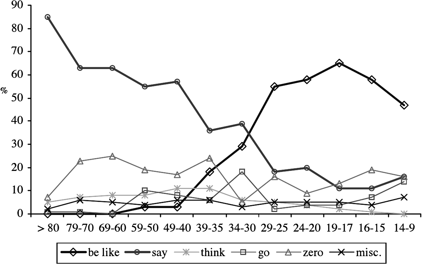
When we ran simulations of this model, we indeed found that an adolescent peak frequently occurred in apparent time curves generated from the simulations.Footnote 2 An example is shown in Figure 6. If we look closely at the trajectory of each cohort, we see that they begin with a usage below that of the leading cohort, before catching up, overtaking to become the leaders, and then falling behind each subsequent cohort. This progression produces the adolescent peak in the apparent time curve. For comparison, in Figure 7 we give the graph of apparent time with the adolescent peak for the quotative be like in Toronto (Tagliamonte & D'Arcy, Reference Tagliamonte and D'Arcy2007:205, Figure 2).
Figure 6. (a) Population mean (heavy black line) and cohort mean usage of the incoming variant over time for a typical simulation realization of the adolescent peak model. (b) The apparent time curve (cohort mean values for the same realization, plotted as a function of age at the time shown by the vertical red dashed line on the left) for the realization exhibits an adolescent peak. (Note: Color images can be viewed online at http://cambridge.journals.org/LVC.)
Figure 7. Toronto quotatives in apparent time (Courtesy of Tagliamonte & D'Arcy, Reference Tagliamonte and D'Arcy2007:205, with thanks to Sali Tagliamonte).
In Figure 8 we plot apparent time curves at multiple real time points through the change. The peak is less prominent at the beginning and end of the change (lowest and highest curves in Figure 8) and most prominent in the middle of the change, when the rate of change is fastest. This is consistent with the observations of Tagliamonte and D'Arcy (Reference Tagliamonte and D'Arcy2009) that we noted earlier. Tagliamonte and D'Arcy also suggested that more rapid changes should exhibit a stronger peak, and this is again observed in our simulations. We measured the difference in usage of the incoming variant between the youngest and second youngest 10-year cohorts at each time during the change and recorded the largest difference observed. We repeated this for simulations using several different replicator selection strengths b to control the speed of the change.
Figure 8. Apparent time curves taken at multiple time points through the same simulation run of the adolescent peak model.
In Figure 9 we plot the maximum peak height (the maximum difference between the mean usage of the first two cohorts) against the time of the change (time taken for the population usage to go from 20% to 80%). Measurements were averaged over 10 repetitions.
Figure 9. Size of the adolescent peak, calculated as the maximum difference between youngest two cohorts in each simulation, averaged over 10 realizations, as a function of the time taken for the community change. (Note: Color images can be viewed online at http://cambridge.journals.org/LVC.)
To understand how frequently and consistently the adolescent peak appears, we repeated the simulation 100 times with the same parameter settings. For each realization, we measured the difference in usage between the youngest two cohorts at multiple times throughout the change. These results were filtered to only include times when the second youngest cohort had a usage between 30% and 70%, so as to avoid times when the usage was very small or very large, as the adolescent peak is much less prominent in these circumstances, because most speakers, young and old, have similar usage patterns. A histogram of the resulting measurements is shown in Figure 9. Positive values correspond to an adolescent peak (second cohort leading first cohort). We see that an adolescent peak appears very frequently, in about 70% of cases, with the average difference being 5.1%. Conducting a two-tailed t-test comparing this mean value to zero, we found p < .00001, meaning that the second youngest cohort lead over the youngest is statistically significant (see the Appendix). For comparison, in Figure 10 we also plot the distributions of differences between the second and third and the fourth and third cohorts. These differences have means significantly less than zero, the t-tests giving p-values of .0008 and <.00001 respectively for the difference from mean zero. That is, from the second cohort onward, the younger cohort leads, as would be expected for a simple S-curve pattern. These results confirm that our hypothesized mechanism of the child being at first overwhelmingly exposed to the caregiver's system, and not the language behavior of other members of the speech community is sufficient to produce the observed adolescent peak.
Figure 10. Distribution of differences in mean usage between the second youngest and youngest cohorts (C2–C1), for 100 realizations of the adolescent peak model using the same parameters (b = .05, H = .05). The mean value is marked with a vertical line. For comparison, the third to second (dashed) and fourth to third (dotted) difference distributions are also shown. (Note: Color images can be viewed online at http://cambridge.journals.org/LVC.)
These experiments were all carried out with an exponentially decaying λ. If instead the power law function is used, an adolescent peak is still observed, as can be seen in Figure 11.
Figure 11. Apparent time curves for the adolescent peak model under the power law λ decay function, observed at three times during the same simulation realization. The adolescent peak also appears when using the power law λ decay function.
We now examine the robustness of these results, by considering variations of several aspects of this model, in order to see whether the absence of any of them also destroys the adolescent peak effect. Keeping the network development the same (i.e., new speakers initially speak exclusively to a single “caregiver,” and gradually add new contacts through their lifetime), we tried choosing the first primary contact in different ways.
First, we tried the case in which a speaker's first primary influence was a “peer”—a speaker chosen with an age in a much younger window, 1 to 15 years old. In this case the adolescent peak effect is essentially removed, and instead the youngest cohort is almost always leading. In the same statistical analysis, the youngest cohort led 63% of the time, with a mean difference of −1.5% which gave a p-value of .38 in a two-tailed t-test, meaning the difference is not significantly different from zero. The distribution of peak sizes is shown in Figure 12. If instead we choose the primary influence to be even older than in our first model, the adolescent peak becomes larger. With primary influence chosen in the age window 30 to 45 years, the second cohort led 81% of the time, with an average difference in usage of 8.2%. Again the presence of the adolescent peak is significant (p < .00001).
Figure 12. Distributions of differences C2 to C1 for the main adolescent peak model (top left) compared with five other variations of the model. Middle left: main influence chosen to be 30 to 45 years old. Lower left: main influence chosen randomly from the entire population. Top right: main influence chosen to be 1 to 15 years old. Middle right: fixed network with the same structure as the adolescent peak model. Lower right: a fully connected network. (Note: Color images can be viewed online at http://cambridge.journals.org/LVC.)
We next tried choosing the caregiver at random from the whole population, rather than from a specific age window. The majority of speakers in the population are adults whose usage lags behind the leading teenagers at any given time, so adopting the system of a randomly chosen contact will generally cause the child to adopt an “old” level of new variant usage. The resulting distribution of peak sizes is also shown in Figure 12. An adolescent peak still occurs and is on average even larger (10.1%) than any of the previous models. Once again, the t-test for the difference from zero gave a p-value of <.00001.
Because a cohort trajectory averages over multiple speakers, the overall effect is very similar to that if all children chose a middle-aged caregiver. This indicates that the exact age of the caregiver is not important to produce an adolescent peak, so long as they are an adult that is no longer in a leading cohort.
Next, we relaxed the condition that a child speaker should interact primarily with a single speaker in the first years of life. We ran the model again, with the same overall pattern of connections in the population as a whole, but now this contact network was fixed, and speakers were randomly assigned a position in the network. This means that new speakers generally have multiple interlocutors, and some adults have only one. Surprisingly, even this randomized model frequently produced an adolescent peak, although somewhat more variably than in the previous cases. The second cohort led 65% of the time, with an average difference between the first two cohorts of 3.7%. The appearance of the adolescent peak even in this model is statistically significant, with the t-test comparison with a mean of zero returning a p-value <.00001.
Finally, we compared the statistics for the original model, with every speaker speaking equally frequently to every other speaker. This model has no special network features designed to produce an adolescent peak. We found that even in this case, an adolescent peak appears, and very frequently. For parameters chosen to give a similar rate of change to that seen in the other model variations, the adolescent peak appeared 88% of the time, with a mean difference between the first two cohorts of 7.8%. Once again, a t-test shows this to be significant (p < .00001).
As for the randomly chosen caregiver model, in these last two cases, a young speaker receives input from a broad range of speakers of differing ages. Together, these provide a usage pattern similar to the population average, which naturally lags behind the leading cohorts. These results show that this average influence is sufficient to produce an adolescent peak. We performed a Welch's t-test to compare the mean difference between the youngest two cohorts with that found in the main model. In the models with older caregiver, randomly selected caregiver, and with a fully connected network, the mean difference between the first two cohorts was larger than that found in the main model, and the difference was found to be statistically significant, with p-values of <.003 (see the Appendix). Only the static network returned smaller adolescent peaks. The main statistics of the adolescent peak for these model variations are given in the Appendix.
We conclude that the adolescent peak appears robustly whenever a child is exposed exclusively or even simply on average to the speech patterns of adults (older than the critical period). Exclusive exposure to peers is sufficient to remove the adolescent peak effect, and in fact appears to be the only means to do so.
TWO PATTERNS OF LANGUAGE CHANGE ACROSS THE LIFESPAN
Evidence and explanations for the two patterns
In the preceding sections, we described well-known, empirically observed patterns of language change across the lifespan that are directly connected to the course of language change in the community: the apparent time construct and the adolescent peak. We showed that these patterns can be modeled with quite simple assumptions based on the results of prior work on the mechanisms of community change (Baxter et al., Reference Baxter, Blythe, Croft and McKane2009; Blythe & Croft, Reference Blythe and Croft2012). In this section, we describe a pattern of language change across the lifespan that has been observed but not (yet) attracted much attention. We show that this pattern also can be accounted for in a simple fashion in our model, but using another variable, one that represents the degree of accommodation of a speaker to her interlocutors in the community.
We discussed the observation that speakers may continue to change their variable linguistic behavior in adulthood. Usually (though not always), this change is in the direction of the community change. In most cases, the change in linguistic behavior in adulthood is relatively gradual. However, results from the largest panel study that describes each individual's trajectory of change, Sankoff and Blondeau's (Reference Sankoff and Blondeau2007:580) analysis of Montréal /r/ in 1971 and 1984, show a different pattern: “this change differs from others described in the literature in one important way: the relative lack of stable variation. More speakers tended to be categorical than variable, and those who changed did so very rapidly.” Specifically, 10 speakers were near categorical (≥83%) in their use of the outgoing variant [r], and 10 speakers were near categorical (≥85%) in their use of the incoming variant [R] (Sankoff & Blondeau, Reference Sankoff and Blondeau2007:571); of the 12 remaining speakers in the panel, 9 increased their use of [R] between 1971 and 1984 to a significant degree (the increase in use ranging from 17% to 74%; the other 3 increased or decreased their use to a nonsignificant degree).
Sankoff and Blondeau (Reference Sankoff and Blondeau2007) contrasted this pattern of little change or categorical change in Montréal /r/ across the lifespan to gradual changes across the lifespan for vowels in the Atlas of North American English (Labov, Ash & Boberg, Reference Labov, Ash and Boberg2006). They suggest that the sharp changes across the individual lifespan may be due to the fact that a change in the pronunciation of /r/ does not have as great an effect on the phonological system as the North American vowel shifts, which are often chain-shifts involving multiple vowel phonemes (Sankoff & Blondeau, Reference Sankoff and Blondeau2007:580–581). However, as we have observed, there are many examples of adult change in a variety of morphosyntactic as well as phonological variables whose systemic effects appear to be variable; and there seems to be no pattern to the magnitude of changes. Admittedly, these other cases of changes in adult lifespans are reported as averages over panels, or averages over speakers in a trend study. For these, an average of gradual change by adult cohorts might hide major shifts by individuals, but this would only be true if some speakers are changing strongly away from the incoming variant, which we saw was rare (see the apparent time construct section). And an average of major change by adult cohorts would mean that at least some individual speakers are substantially changing the proportion of their use of a linguistic variant across at least part of their adult lifespan. Hence, it may not be the case that the trajectory of individual changes in linguistic behavior for a community change in progress is attributable to the role of the linguistic variable in the linguistic system.
Nevalainen and colleagues also compared individual change to community change in real time in the Corpus of Early English Correspondence ([CEEC], Nevalainen & Raumolin-Brunberg, Reference Nevalainen and Raumolin-Brunberg2003; Nevalainen et al., Reference Nevalainen, Raumolin-Brunberg and Mannila2011). They also observed that in some changes a greater proportion of speakers are relatively more categorical (their “progressive” and “conservative” categories) than the remaining speakers (their “in-between” category). They compared the shift from negative concord to sentential negation with an indefinite and the shift from the gerund in -ing with an object introduced by of to an object without of; the former shift has many fewer in-betweens than the latter shift (Nevalainen et al., Reference Nevalainen, Raumolin-Brunberg and Mannila2011:25). They argued that the rate of change contributes significantly to this difference: faster changes, such as the shift away from negative concord, leads to fewer in-between speakers than slower changes such as the shift to a gerund with a direct object (Reference Nevalainen, Raumolin-Brunberg and Mannila2011:25, 35).
Modeling the two patterns of language change across the lifespan
We agree with Nevalainen et al. (Reference Nevalainen, Raumolin-Brunberg and Mannila2011) that the rate of change plays a significant role in the different distribution of individual behavior that is observed. However, we propose that the differences are due not only to the relative weighting of the linguistic variants (that is, b), a primary determinant of the rate of change, but also to a second social variable: the degree that a speaker accommodates to other speakers in the community (that is, H). A speaker who accommodates more easily to other speakers will undergo change gradually, trending toward the community mean for the variant at a given point in time. A speaker that accommodates less easily to other speakers will retain the outgoing variant, and if and when she does change to the incoming variant, will do so rapidly. These two patterns of individual accommodation lead to two different distributions of individual behaviors at different stages of a community change.
By varying the value of H, we can explore these different patterns of change in our model. In Figure 13 we show some examples of different cases. The solid black lines represent the average usage over the whole population, while the dots are the usage of a small number of randomly sampled speakers at multiple times. In all cases, the overall mean population usage of the incoming variant follows a smooth S-curve. However when H is small, as in the left-hand plot, speakers cluster near categorical usage of one or other variant (the distribution between them determining the population mean). On the other hand, when H is large, as in the right-hand plot, individual speakers change more smoothly through variable usage, more closely following the population-wide S-curve. The middle plot illustrates a case between these two extremes, with still a large number of categorical speakers, but also a significant number with mixed usage.
Figure 13. Change in individual “categoricalness” as accommodation increases. From left to right, H = .006, .014, .022, for fixed replicator selection strength b = .01. Solid lines give population mean grammar over time. Dots are grammars of 20 randomly sampled speakers from a population of 1000 (different sample at each time). (Note: Color images can be viewed online at http://cambridge.journals.org/LVC.)
The difference between the patterns is most evident in the middle of the change. At the beginning and end of the change, the whole population uses a large fraction of either the old variant or the new one, and so necessarily all speakers will also have near-categorical usage. This can be seen clearly when we consider the development over time of the standard deviation of the individual speaker usage, as plotted in Figure 14. The standard deviation is very small at the beginning and end of the change and is largest in the middle. A peak standard deviation above about .29 indicates a polarized pattern, with speakers clustered near the boundaries (as seen in the left-hand plot, which is for a small value of H). A peak standard below this value indicates that speakers are centrally clustered, as seen in the right-hand plot (for large H). The boundary value .29 is simply the standard deviation we would find if speakers were uniformly distributed across the whole range from 0% to 100%. We also calculated the standard deviation separately for speakers 0 to 20 years of age (blue line) and 40 to 60 years of age (green line; color online only). For small H, the curves are very similar to the overall population curve, though peaking a little earlier for young speakers and a little later for older speakers. When H is large, however, we see that the youngest speakers are more diverse, and the older speakers are more homogeneous than the population as a whole.
Figure 14. Standard deviation of population grammar values over time. (a) For a small value of the accommodation parameter H, resulting in a polarized pattern of change. (b) For a large value of H, resulting in a centralized pattern of change. Black line and circles are for the whole population. Blue dash-dot line: speakers 20 years old or younger. Green dashed line: speakers 40 to 60 years old. (Note: Color images can be viewed online at http://cambridge.journals.org/LVC.)
Interestingly, the values of H for which we see the different patterns also depend on the strength of replicator selection (b). We can understand this in the following stylized way. Speakers encounter two conflicting forces. Replicator selection drives them toward categorical usage of the new variant, and accommodation drags them toward the average usage of their interlocutors. For the distribution of speaker grammars to be centralized, the accommodation parameter H must be large enough to overcome not only a speaker's natural tendency toward categorical behavior but also the force of replicator selection b. This pattern is summarized in Figure 15a for the exponential λ decay function (2). The degree of polarization, as measured by the population standard deviation at the midpoint of the change, is indicated by the color in the plot, with blue representing small standard deviation, that is, the centralized pattern, and orange-red representing large standard deviation, the highly polarized pattern of change (color online only). The thick red line represents the crossover value .29. We see that for larger b, the value of H needed to reach the centralized pattern also increases.
Figure 15. Summary of variation in patterns of change with the main parameters b and H, (a) using the exponential λ decay function, (b) using the power law λ decay function. Shading indicates population variance, dark smallest and light largest values, corresponding to centralized and polarized patterns of change, respectively. The red line marks the boundary value, variance = 1/12 (standard deviation = .29). White curves indicate lines of equal time of change, with value (in years) labeled. Pink circles mark the parameter values for simulations most closely resembling study data, as discussed in the text. (Note: Color images can be viewed online at http://cambridge.journals.org/LVC.)
Varying the parameters b and H also has an effect on the time taken for the change. As we might expect, the strength of the replicator selection b has the strongest effect. Increasing b increases the tendency of speakers to produce the incoming variant, leading to faster adoption. However, for a given value of b, changing H also affects the time taken for the change, with stronger accommodation (larger H) corresponding to longer times, as the tendency of younger speakers to switch over rapidly to use of the new variant is held back by the influence of older speakers still using the old variant. The times taken for the change are indicated in Figure 15a by white lines tracing contours of equal change time. The shortest times occur in the lower-right region of the plot, and we see that there is a minimum time for a change of approximately 60 years. This is due to the aging of the speakers. The change cannot be completed while there are older, inflexible speakers still using or partly using the original variant. In this region, then, the change time becomes independent of the model parameters and depends only on the demographics of the population. The same effect can be observed in Figure 4a, in which the apparent time for the change (corresponding to the leading cohort of young speakers) can take very small values, but the real time for the change reaches an asymptotic value. This effect still occurs even when adult speakers are still able to change somewhat, as shown in Figure 15b, which was generated using the power law λ decay function (3) with γ = 2.
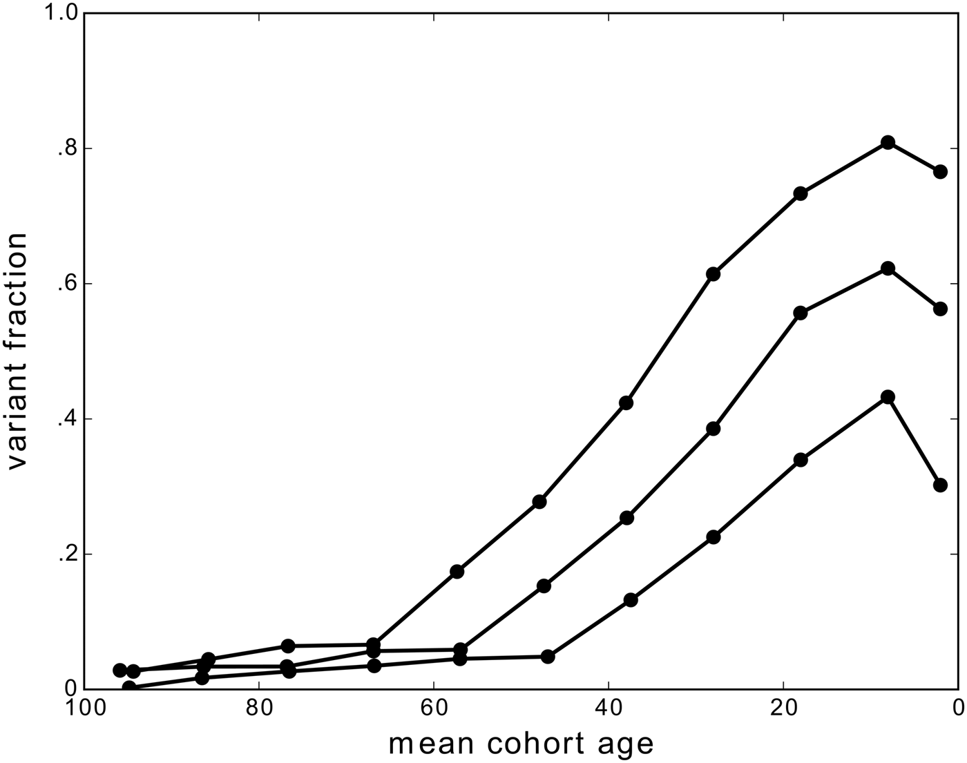
The most detailed published data of the distribution of individual linguistic behaviors at different stages of a community change is for the CEEC. Nevalainen and Raumolin-Brunberg (Reference Nevalainen and Raumolin-Brunberg2003:101–109, Appendices 5.1–5.3; see also Raumolin-Brunberg, Reference Raumolin-Brunberg2005) gave percentages of use of the incoming variants by individuals in the CEEC for three changes: 3rd person -th to -s, 2nd person subject pronoun ye to you, and relativizer the which to which (only individuals for whom there were at least 10 tokens in the 20-year time intervals used were included; Nevalainen & Raumolin-Brunberg, Reference Nevalainen and Raumolin-Brunberg2003:92). The last change is more complex than the first two, in that the which and which were not only competing with each other, but both were competing with the outgoing WH-Prep (e.g., whereby), and themselves occurred in two variants for prepositional relatives (preposition before which/the which vs. stranded preposition). For this reason, we excluded the which/which from analysis. For the community change, published numerical data is available for the 3rd person singular verb form and 2nd person pronoun (Nevalainen, Reference Nevalainen, Bermúdez-Otero, Denison, Hogg and McCully2000:360, Tables II and III). The -s/-th and you/ye changes are rapid, so we compare them to individual data on the slower change to gerund plus direct object generously provided to us by Nevalainen and Raumolin-Brunberg (data on the community change for gerund plus direct object is found in Nevalainen and Raumolin-Brunberg [Reference Nevalainen and Raumolin-Brunberg2003:66, 219]).
As we established in simulations, the peak value of the standard deviation of individual usage can be used as an indicator for the different patterns of change. In Figure 16a we plot the overall mean proportion of -s for each of the 20-year time intervals from 1560 to 1659 (circles). We also plot the standard deviation of the individual usage for each window (triangles). Just as in the model, the standard deviation rises to a peak at about the midpoint of the overall S-curve, before reducing again as the change nears completion. In this example, the peak standard deviation value is about .33, indicating that this change is of the polarized type. The solid curves in the figure are model outputs. Model runs were carried out at a range of parameter settings (b and H), and the output most closely resembling the standard deviation and time of change of the data was chosen. The parameters corresponding to this particular choice are indicated in Figure 16a. The agreement with the standard deviation curve is excellent, and the S-curve is quite well fitted. Similar results were obtained using the power law λ decay function. The agreement of the model with data is seen even more clearly in Figure 16b, where we plot the distribution of individual speakers (gray bars) at different times through the change, along with the corresponding population distribution found in the model. In particular, the weakly polarized distribution in the middle of the change is well predicted by the model (solid curves). To quantify the agreement, we performed double sample Kolmogorov-Smirnov tests (Massey, Reference Massey1951) for agreement between the two distributions at each time point. We found no evidence at any of the five time periods to reject the hypothesis, at the 99% level, that the two distributions (the model curve and the sample distribution) are the same.
Figure 16. (a) Time evolution of population usage of -s (circles) and standard deviation (triangles). Solid and dashed lines are matching simulation values. (b) Distribution of individual usage of -s in the population at several times through the change. Gray bars show density of speakers in the given interval, taken from data. Blue lines are the equivalent densities for matching simulation. (Note: Color images can be viewed online at http://cambridge.journals.org/LVC.)
The data for you/ye are not as clear, with the standard deviation fluctuating rather than following a smooth curve; see Figure 17a. Nevertheless, we estimated the peak standard deviation to be about .38, suggesting an even more polarized pattern of change than -s/-th. The simulation curve cannot be as closely matched; nevertheless the predicted highly polarized distribution, now found at several intervals throughout the change, once again matches the distribution of speaker usages quite well; see Figure 17b. We repeated the Kolmogorov-Smirnoff tests. For the first four time periods we found no evidence to reject the hypothesis, at the 99% level, that the two distributions are the same, while for the fifth time period this hypothesis was rejected at the 95% level.
Figure 17. (a) Time evolution of population usage of you/ye (circles) and standard deviation (triangles). Solid and dashed lines are matching simulation values. (b) Distribution of individual usage of you/ye in the population at several times through the change. Gray bars show density of speakers in the given interval, taken from the data. Green lines are the equivalent densities for the matching simulation. (Note: Color images can be viewed online at http://cambridge.journals.org/LVC.)
The data for the gerund plus direct object change are even more difficult to fit. Data were available for 20-year intervals from 1440 until about 1680, but there is a great deal of fluctuation in the early part of the change, in large part due to the very small number of speakers recorded in those years. For this reason we chose to only fit the data from 1540 to 1559 onward, from which time the curve is more stable. At this point the average usage had already reached around 30%. The S-curve appears to saturate at around 80%, a possibility that is not catered for in the model (see Figure 18a). Furthermore, this causes the peak standard deviation in our fitted curve to occur at a different time to that in the data.
Figure 18. (a) Time evolution of population usage of gerund plus direct object (circles) and standard deviation (triangles). Solid and dashed lines are matching simulation values. (b) Distribution of individual usage of gerund plus direct object in the population at several times through the change. Gray bars show density of speakers in the given interval, taken from data. Magenta lines are the equivalent densities for matching simulation. (Note: Color images can be viewed online at http://cambridge.journals.org/LVC.)
A further caveat in this example is that the distribution for such centrally peaked changes will be different for speakers of different ages. Assuming the authors in the CEEC are all adults, the population standard deviation including children as well may well have a slightly higher peak. Nevertheless, we were able to find simulation curves that approximately matched the data. The largest standard deviation value observed, .26, is just below the threshold of .29, meaning that there is a significant fraction of mixed-usage speakers throughout the change. The histograms of individual usage are again well matched by the model simulation curves. Repeating once again the two distribution Kolmogorov-Smirnoff tests, we found that for the first six time periods, there was no evidence to reject the hypothesis that the two distributions are the same, at the 99% level. However, in the last time period, the hypothesis was rejected at the 90% level. We see indeed that the speakers are mostly in the middle of the range in the intervals 1580 to 1599 and 1600 to 1619, indicating that this change is a different pattern from the previous two.
Our statistical tests showed that our model gives a good match to the data in 15 of the 17 time periods studied. These results show that our simple model not only captures the correct shape of the distribution of speaker usage at a given time, but also captures the evolution of this distribution over time, for both the polarized and centrally peaked patterns of change.
A final example is available in Sankoff and Blondeau's (Reference Sankoff and Blondeau2007) study of Montréal /r/ in 1971 and 1984. These panel studies tracked the changes in individual speakers. Nevertheless, we can estimate the population distribution of usages from the usages of the 36 speakers in each of the two surveys. Exact usage proportions were available for nine highly variable speakers who had intermediate usage at one or both times. The ages and usage percentages for the remaining speakers were estimated visually from Sankoff and Blondeau (Reference Sankoff and Blondeau2007:572, Figure 3). An apparent time S-curve for the change was derived using data from Sankoff, Blondeau, and Charity (Reference Sankoff, Blondeau, Charity, Van de Velde and van Hout2001).
The standard deviation for the speakers in the 1971 study for which we have individual data is .39, while for 1984 data it was .40. If instead we divide the speakers into age cohorts, and find the standard deviation for each cohort, the largest standard deviation was for speakers born between 1937 and 1951, being .43 for the 1971 data or .44 for 1984 data. All of these values are far above the threshold value of .29, meaning that this example is the most polarized of the four we have described. This is clear from the individual data, in which 23 of the 36 individuals had near-categorical usage of one variant or the other both in 1971 and 1984.
As we have already observed, apparent time curves tend to underestimate the duration of a change. Looking back at Figure 4a, we see that an apparent time change over 30 years corresponds to a real time change of 50 to 60 years. The best-match model parameters were found by calculating apparent time curves from the simulations and matching them to the Montréal apparent time data. The result is shown in Figure 19. The red curve is apparent time, the black dotted curve is real time, and both are from the simulation (color online only). Also plotted is the evolution of the standard deviation, which also roughly matches the data. This example corresponds to the pink dot marked on the contour diagram in Figure 15a. Due to the fact that the curve from the Montréal study involves a small number of speakers, divided across several cohorts for an apparent time curve, and due to the extraction of apparent time curves from simulation data, the uncertainties in the shape of both real data and simulation curves are much larger than in the previous examples. The best fit simulation parameters could therefore only be chosen approximately, and we did not perform statistical goodness-of-fit tests for this case.
Figure 19. Simulation match to Montréal /r/ data. Circles are apparent time data from 1971, triangles are standard deviation values for the same. Solid orange line is the mean grammar value of the leading cohort for a simulation realization using the best matched parameters. Dashed line is standard deviation of leading cohort. For comparison, the real time whole population curves (grammar and standard deviation) from simulation are also plotted (thin solid and dotted curves). (Note: Color images can be viewed online at http://cambridge.journals.org/LVC.)
The parameters corresponding to the best matches to the four data sets discussed are marked by pink circles in Figures 14a and 14b. We see that they all fall in different areas of the plane, with the gerund plus direct object change falling on the centrally peaked part of the diagram, and the others falling in the region corresponding to the polarized pattern. There seems to be no particular pattern to their positioning. In particular, the s/th, you/ye, and gerund plus direct object changes, the data for which all come from the same corpus, and hence occurred in the same population, agree neither in the value of H or in b.
We note also that the contours of time-of-change run almost parallel to the contours of the population standard deviation across a large part of the diagram. In particular, more centrally peaked areas tend to have longer times than more polarized areas, in agreement with the observation of Nevalainen et al. (Reference Nevalainen, Raumolin-Brunberg and Mannila2011). However we disagree as to the cause: it is not that faster changes cause more polarization, but that the parameters leading to faster changes also happen to lead to more polarization.
CONCLUSIONS
We have shown that a number of different mechanisms of language change in the model used here are responsible for different phenomena that have been observed in community change and in individual change across the lifespan. The most general property of community change across time, the S-curve, is determined by replicator selection, that is, differential weighting of variants of a linguistic variable, following the classic Labovian model (Blythe & Croft, Reference Blythe and Croft2012). Under that umbrella of community change, a number of mechanisms interact to bring about variation and change across the individual lifespan. Our model offers another means to evaluate qualitative explanations that have been offered for individual change that cannot be practically tested (or cannot be tested at all) in a real world, large-scale speech community.
The apparent time construct has been explained in terms of a decline in flexibility in adopting novel variants, or frequencies of novel variants in appropriate linguistic and sociolinguistic contexts, as a speaker ages. We modeled this decline in flexibility with a gradual function that declined rapidly around adolescence or early adulthood. The results straightforwardly confirmed the basic account of the apparent time construct. Of course, adults are able to alter their linguistic behavior to some degree. We have accommodated for this possibility by using a decay function that allows some adult change. To model the specifics of such changes will require developing a model of social differentiation within a speech community; we have not done this here, although it is an avenue for future research.
The two patterns of individual change (more centralized and more polarized), observed by Sankoff and Blondeau (Reference Sankoff and Blondeau2007) and by Nevalainen et al. (Reference Nevalainen, Raumolin-Brunberg and Mannila2011) were explained by Nevalainen et al. as a consequence of the rate of change in the linguistic variable. While we agree that there is a correlation between the pattern of change and the rate of change for a linguistic variable, our model suggests that the correlation and the two patterns can be explained by the interaction of the differential weighting of the variants and the degree of accommodation of speakers. Speakers who accommodate more readily to their interlocutors will change more continuously (the centralized pattern), while speakers to accommodate less readily will change more suddenly, if they change at all (the polarized pattern).
Perhaps the most interesting result of the model has to do with the explanation for the adolescent peak. The adolescent peak has been explained as a consequence of a child being exposed to older caregivers before associating more widely with older peers and incrementing their language use correspondingly. This can be modeled in terms of a specific dynamic network structure: a child interacts with her caregivers at first, then gradually comes to interact with more members of the speech community. In fact, however, the adolescent peak results from any network model in which a child is exposed to adult speakers of any age; only if the child interacts solely with caregivers in the adolescent cohort does the adolescent peak disappear. On the one hand, this might be a more realistic model of children's interactions: they interact with a wider range of speakers, including adults of differing ages, from early in childhood. On the other hand, it might suggest that at least for this phenomenon, social network structure does not play a significant role in bringing it about.
The model used in this analysis does not include socially structured variation in linguistic behavior. Socially structured variation is also found across an individual lifespan, as a speaker undergoes changes in social role and in the social networks that she is engaged in (see Bailey [Reference Bailey, Chambers, Trudgill and Schilling-Estes2002], referring to an unpublished 2000 study by Cukor-Avila; Cukor-Avila [Reference Cukor-Avila2002]; De Decker [Reference De Decker2006]; Eckert [Reference Eckert and Coulmas1997, Reference Eckert2000]; Pritchard & Tamminga [Reference Prichard and Tamminga2012]; Wagner [Reference Wagner2012b]). These changes in linguistic behavior appear to involve the manipulation of linguistic variants for social purposes even when the variation is stable at the community level (age-grading in the narrow sense; Wagner, Reference Wagner2012b), or the status of the variation at community level is unclear (Cukor-Avila, Reference Cukor-Avila2002), as well as cases of variants undergoing community change. That is, it appears that these age-related changes reflect linguistic effects of variation in social identity and social network across a speaker's lifespan, whether or not the variation is part of a community change in progress.
The model presented here is relatively simple in terms of the number of variables and mechanisms of interaction, variation, and change posited. Yet it is able to model the interplay between community change and individual change across the lifespan. It is also able to model relatively fine-grained phenomena such as the adolescent peak and the two patterns of language change described. As such, it suggests that there can be a fruitful marriage of empirical sociolinguistic research with mathematical modeling of proposed explanations for sociohistorical linguistic variation and change.
APPENDIX
Statistics of adolescent peak for several model variations