


1 Introduction.
Imagine that you are offered the choice between two wheels of chance, as displayed in Figure 1. The chosen wheel of chance, in such a gamble pair, if played for real money, will be spun. If the black part of the wheel is oriented towards the Dollar amount when it stops (which is the case in both wheels as displayed in Figure 1) then you win the indicated amount, otherwise nothing. In the left gamble of Figure 1 you can win $25.2 (with 37.5% chance), whereas in the right gamble you can win $22.4 (with 48.8% chance). As the screenshot shows, the numerical probabilities of winning are not provided. The decision maker depends on the relative size of the black shaded area to evaluate the chance of winning. When offered such stimuli repeatedly, decision makers tend to fluctuate in the choices they make. For over 50 years, it has been a point of debate how one can model choice variability formally. A natural approach is to model choice behavior probabilistically.
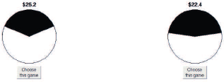
Figure 1: Screen shot of a Cash I paired-comparison stimulus (see also RDDS, Figure 2)
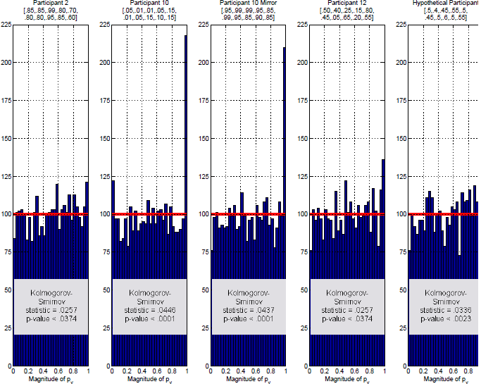
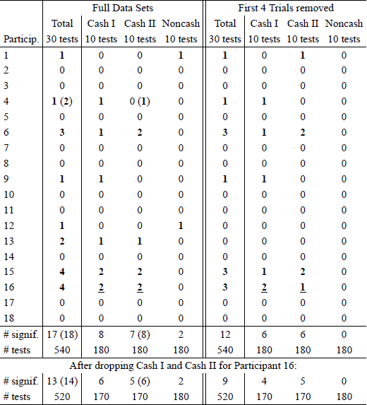
Figure 2: Illustrative analysis of the sampling distribution of p ν approximated through 3,000 simulated iid data sets using the maximum likelihood binomial parameters of three participants from Regenwetter et al. (2011) Cash I, and a hypothetical participant. The underlying binomial probabilities are given above the histograms. The expected frequency in each bin under the uniform null is given by the horizontal line. The Kolmogorov-Smirnov statistic is significant in each case, i.e., each distribution differs significantly from a uniform on [0,1].
Reference Regenwetter, Dana and Davis-StoberRegenwetter, Dana and Davis-Stober (2010, 2011) [henceforth RDDS] investigated a mathematical model of binary choice probabilities with a distinguished history in economics, operations research, and psychology, whose mathematical structure has been studied intensely over several decades (see, e.g., Reference Becker, DeGroot and MarschakBecker, DeGroot, & Marschak; 1963, Reference Block, Marschak, Olkin, Ghurye, Hoeffding, Madow and MannBlock & Marschak, 1960, Reference Bolotashvili, Kovalev and GirlichBolotashvili, Kovalev, & Girlich, 1999; Reference Cohen and FalmagneCohen & Falmagne, 1978, 1990; Reference FioriniFiorini, 2001; Reference FishburnFishburn, 1992; Reference Fishburn and FalmagneFishburn & Falmagne, 1989; Reference GilboaGilboa, 1990; Reference Grötschel, Jünger and ReineltGrötschel, Jünger & Reinelt, 1985; Reference Heyer and NiederéeHeyer & Niederée, 1992; Koppen, 1991, 1995; Reference Marschak, Arrow, Karlin and SuppesMarschak, 1960), but for which there did not previously exist an appropriate statistical test. This model has been studied under several labels, including “binary choice model”, “linear ordering polytope”, “random preference model”, “random utility model” and “rationalizable model of stochastic choice”, and it has been stated in several different mathematical forms that make the same empirical predictions (see, e.g., Reference Fishburn, Barbera, Hammond and SeidlFishburn, 2001; Reference Regenwetter and MarleyRegenwetter & Marley, 2001). We will refer to it as the linear order model. According to this model, preferences form a probability distribution over linear orders, i.e., over rankings without ties. The probability that a person chooses one gamble over another is the probability that s/he ranks the chosen gamble higher than the non-chosen gamble. Denote the probability that a person chooses x (say, the left gamble in Figure 1) over y (say, the right gamble in Figure 1) as Pxy. The linear order model makes restrictive predictions: It requires that the triangle inequalities hold, according to which, for all distinct choice options a, b, c,
This model has a particular mathematical form that long eluded statistical testing: For inequality constraints like these, standard likelihood ratio tests are not applicable, goodness-of-fit statistics need not satisfy the familiar asymptotic χ2 (Chi-squared) distributions, and it is not even meaningful to count parameters (e.g., binary choice probabilities) to obtain degrees of freedom of a test. Formally adequate statistical tests for such models have been discovered only recently (Reference Davis-StoberDavis-Stober, 2009). Reference Regenwetter, Dana and Davis-StoberRegenwetter, Dana and Davis-Stober (2010, 2011) were the first to carry out such a state-of-the-art “order-constrained” test of the linear order model. Even breakthrough results come at a price: To our knowledge, there does currently not exist a statistical test for the triangle inequalities that does not assume iid (independent and identically distributed) sampling of empirical observations.
Notice that the triangle inequalities (1) make no mention of time, of the individual making these choices, or of repeated observations. They do not require binary choice probabilities to remain constant over time or be the same for different decision makers (i.e., they do not require an identical distribution), nor do they require binary choices to be made stochastically independently of each other (see Regenwetter, submitted, for a thorough discussion). Reference BirnbaumBirnbaum (2011, 2012) [henceforth MB] has questioned the iid sampling assumption used by RDDS’s statistical test and recommended his own models, the so called “true-and-error” models, as an alternative. Regenwetter (submitted) shows that MB is mistaken to attribute the iid assumption to the linear order model itself, i.e., to the triangle inequalities (1). Among the leading models of probabilistic choice, the linear order model stands out in being invariant under non-stationary choice probabilities (i.e., invariant under certain violations of the “identically distributed” part of “iid”). Regenwetter (submitted) also shows that, in contrast, a number of published papers on “true-and-error” models do, in fact, require binary choice to be iid in both the model formulation and in the statistical test.
The main concern in this paper, however, is with Reference BirnbaumBirnbaum’s (2012) claim that the iid assumption, used by the state-of-the-art test in RDDS, is violated in the RDDS data. We will first provide a brief introduction to the RDDS experiment, then show that the RDDS data pass a well-known test of iid sampling without a hitch. We then document that Reference BirnbaumBirnbaum’s (2012) proposed tests of iid sampling have unknown Type-I error rates that even appear to change with the way in which binary choices are coded, and do not actually appear to test iid sampling per se. We add to this conclusion the finding that Reference BirnbaumBirnbaum’s (2012) tests fail to replicate within participant. We provide evidence against MB’s suggestion that the excellent model performance in RDDS might be a Type-II error in which warm-up effects could have made binary choice probabilities shift early in the experiment and then choice probabilities violating the model could have accidentally averaged to satisfy the triangle inequalities. Last but not least, we use Reference BirnbaumBirnbaum’s own (2012) hypothetical data to disprove MB’s claim that “true-and-error” models overcome alleged limitations of the linear order model.
2 The experiment of RDDS.
In a seminal paper, Reference TverskyTversky (1969) used a collection of 5 distinct wheels of chance and formed all 10 possible pairs of these gambles. Faced with variability in behavior, he presented each decision maker 20 times with each gamble pair in an effort to assess their preferences among the five gambles from the observed choice proportions. Tversky augmented the set by 10 “irrelevant” distractor pairs, also presented 20 times. In other words, he presented his participants with a sequence of 400 binary choices like the one in Figure 1. The 400 pairwise choices were spread over five weekly test sessions of 80 choices each. RDDS built on this design by asking altogether twice as many pairwise choices, but in a single session and using a computer. They considered three distinct sets of 5 lotteries, as well as some Distractor items. Their Cash I set was the contemporary dollar equivalent of Reference TverskyTversky’s (1969) stimuli, whereas their Cash II and Noncash stimulus sets were new. Like Reference TverskyTversky (1969) they presented each lottery pair 20 times (except for the Distractors, which varied).
Table 1 gives an example summary of the first 36 trials of the RDDS experimentFootnote 1 for Participant #100. On Trial 1, the decision maker faced the choice between a “41.7% chance of winning $23.8” (presented as a wheel of chance on the left side of the screen) and a “33.3% chance of winning $26.6” (presented on the right side). This was a stimulus from the Cash I set. The decision maker chose the gamble presented on the right. On Trial 2, the decision maker was presented with the first of 200 Distractor items, which were intended to interfere with the memory of earlier choices, thus making it difficult to recognize repeated items. Trial 3 involved gambles for non-cash prizes, namely a “24% chance of winning a gift certificate worth approximately 4 music CDs” or a “20% chance of winning a gift certificate for approximately 7 paperback books”.
Table 1: First 36 out of 800 pairwise choices of Participant # 100 in RDDS.
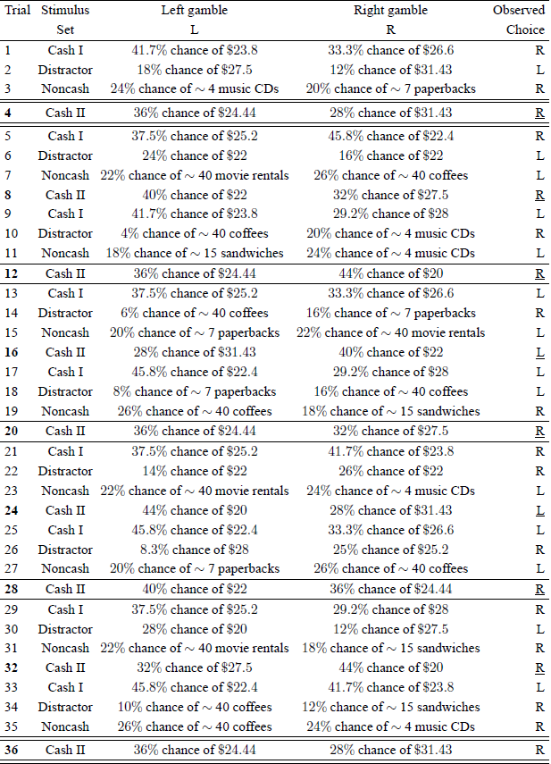
Note: The symbol ∼ stands for “approximately”.
In Table 1, Trials 4, 12, 20, 28, and 36 are set apart by horizontal lines. The lottery with a “36% chance of winning $24.44” was presented in each of these five trials. The side of the screen on which each lottery appeared was randomized. The lottery presentation, unbeknownst to the participant, cycled through the four stimulus sets in the order Cash I, Distractor, Noncash, Cash II. The pair of lotteries presented in a given trial was picked randomly from its stimulus set with the constraint that it had not appeared in the previous five trials from that set; and each individual lottery was chosen with the constraint that it had not appeared in the previous trial from that set. This is why the trials involving a “36% chance of winning $24.44” are separated by at least eight pairwise choices, and why the repetition of the lottery pair in Trial 4 did not occur until at least 24 trials later; in this case, it was in Trial 36.
Many prominent probabilistic models of choice in the behavioral and economic sciences, including the models that Reference TverskyTversky (1969) considered,Footnote 2 assume that the decision maker has a single fixed deterministic preference state throughout the experiment and that variability in observed choices is due to noise or error in one form or another (Reference Becker, DeGroot and MarschakBecker et al., 1963; Reference BirnbaumBirnbaum, 2004; Reference Block, Marschak, Olkin, Ghurye, Hoeffding, Madow and MannBlock & Marschak, 1960; Reference Carbone and HeyCarbone & Hey, 2000; Reference Harless and CamererHarless & Camerer, 1994, 1995; Reference HeyHey, 1995, 2005; Reference Hey and CarboneHey & Carbone, 1995; Reference LoomesLoomes, 2005; Reference Loomes, Moffatt and SugdenLoomes, Moffatt & Sugden, 2002; Reference Loomes, Starmer and SugdenLoomes, Starmer & Sugden, 1991; Reference Loomes and SugdenLoomes & Sugden, 1995, 1998; Reference LuceLuce, 1959; Reference Luce, Suppes, Luce, Bush and GalanterLuce & Suppes, 1965; Reference Marschak, Arrow, Karlin and SuppesMarschak, 1960; Reference TverskyTversky, 1969). The linear order model tested in RDDS models preferences themselves as probabilistic. For example, a decision maker could be uncertain about what he or she prefers on a given trial.
The statistical test currently available for such models requires that one can combine multiple observations together to estimate choice probabilities from choice proportions:
-
1. Writing x for the lottery with a “36% chance of winning $24.44” and y for the lottery with a “28% chance of $31.43,” the statistical test in RDDS treated Trials 4 and 36 as two independent draws from a single underlying Bernoulli process with probability Pxy of choosing x over y.
-
2. Similarly, for two lottery pairs, say, x versus y and a versus b, from the same stimulus set (thus separated by at least 4 trials), the statistical test assumed that those two binary choices were independent draws from two Bernoulli processes with probabilities Pxy and Pab.
Because each stimulus set was analyzed separately, there was no assumption about the relationship between choices from different stimulus sets, say, the choices made on Trials 1 and 2, for instance. The iid assumptions applied only to choices within stimulus set. These two assumptions allow a researcher to use choice proportions as estimators of choice probabilities and this is precisely how they are routinely used in quantitative analyses of probabilistic choice models in psychology, econometrics, and related disciplines. It is the first iid sampling assumption above that MB has questioned. Reference BirnbaumBirnbaum (2012) claims that this iid assumption is violated in the RDDS data. We will now consider the legitimacy of that inference.
3 A test of iid sampling suggested in Reference Smith and BatchelderSmith and Batchelder (2008).
Reference Smith and BatchelderSmith and Batchelder (2008, p. 727) provided a statistical test of iid sampling in binary choice data. Reference BirnbaumBirnbaum (2012) cited Smith and Batchelder but left out any application of their test. We fill this gap by implementing Reference Smith and BatchelderSmith and Batchelder’s (2008) test on the RDDS data. This test uses the analytically derived expected value and standard error of a particular test statistic.
Let (i, i ′) denote some gamble pair. Throughout this section, we will enumerate only the 20 trials that the gamble pair (i, i ′) was presented in RDDS (not the 800 trials of their experiment). So, Trials 4 and 36 in Table 1 become t = 1 and t = 2 for the gamble pair (i, i ′) where i:“36% chance of $24.44” and i ′: “28% chance of $31.43”. For t ∈ {1, 2, …, 20}, let
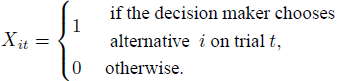
We wish to test, for each gamble pair (i, i ′), whether the Xit result from 20 independent and identically distributed Bernoulli trials, for t = 1, 2, …, 20. By Smith and Batchelder (2008, p. 727), we can consider the following quantity defined in their Eq. 21, which checks for a 1-step choice reversal from trial t to trial t + 1:
Based on this quantity, we consider the number of 1-step choice reversals given by
By Reference Smith and BatchelderSmith and Batchelder (2008), if the 20 Bernoulli trials are independent and identically distributed, i.e., have fixed probability θi of success, we must have
We give a proof in the Appendix. Reference Smith and BatchelderSmith and Batchelder (2008) did not provide a standard error for Ai. We show in the Appendix that the standard error equals
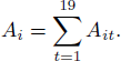
Table 2 shows the results of this test when applied to the RDDS data. For each of the 18 participants in Regenwetter et al. (2011), we carried out 30 tests (for the 30 binomials that RDDS use for each person, 10 for each of Cash I, Cash II, and Noncash) to see whether we may assume, for each of the 30 gamble pairs, iid draws from a fixed Bernoulli process to obtain 30 distinct binomials per respondent. This analysis of iid sampling involved a total of 18 × 30 = 540 hypothesis tests.Footnote 3 We determined confidence intervals using the point estimate given in our Eq. 3 and the standard error, SE(Ai) given in our Eq. 4. We report the number of significant violations (marked in bold) using a margin of error of 2 SE(Ai), or 1.96 SE(Ai) (reported in parentheses, when different).
Table 2: Test of iid binary choice following Eq. 21 and text in Reference Smith and BatchelderSmith and Batchelder (2008, p. 727).
Since we are looking for evidence of mistaken acceptance of the linear order model in RDDS, we also provide an analysis where we leave out the two data sets (Cash I & II, Participant 16) where Regenwetter et al. (2011) already rejected the linear order model (underlined). Rejections by Reference Smith and BatchelderSmith and Batchelder’s (2008, Eq. 21) test occurred at a rate of ∼ 3%, well within standard Type I error range. There is no reason to conclude, based on this test, that the binary choices of each individual in Regenwetter et al.’s (2011) data were anything but independent and identically distributed Bernoulli trials, hence that the choice frequencies originated from anything but Binomials. The null hypothesis of iid sampling in RDDS is retained in this hypothesis test.
4 Type-I error rates of Reference BirnbaumBirnbaum’s (2012) tests.
In contrast to Smith and Batchelder’s test statistic, whose expected value and standard error we reviewed above, Reference BirnbaumBirnbaum (2012) created two new test statistics with unknown sampling distributions. Using these new statistics, Reference BirnbaumBirnbaum (2012) estimated two quantities p ν and pr from the data and, without formal proof, interpreted these quantities p ν and pr as p-values of tests of iid sampling for a given participant in RDDS. Birnbaum concluded that a data set in RDDS violates the iid assumption “significantly” (at an α level of 0.05) when p ν< 0.05, respectively, when pr < 0.05.
To better understand Birnbaum’s test statistics, we can borrow tools from an ongoing debate in the behavioral, statistical, and medical sciences. That debate is primarily concerned about “publication bias”, “p-hacking”, “data peeking”, the “file drawer problem”, etc. (Reference FrancisFrancis, 2012a, 2012b; Reference Ioannidis and TrikalinosIoannidis & Trikalinos, 2007; Reference Macaskill, Walter and IrwigMacaskill, Walter & Irwig, 2001; Reference Simmons, Nelson and SimonsohnSimmons, Nelson & Simonsohn, 2011). We tap into some of the tools with which this literature investigates whether reported p-values match what is expected for a given set of hypotheses and a given effect size. Specifically, we build on the fact that p-values are, themselves, random variables (Reference Murdoch, Tsai and AdcockMurdoch, Tsai & Adcock, 2008). The p-values of a continuous statistic must satisfy a uniform distribution under the null hypothesis, whereas the p-values of finite statistics can display more complicated behavior (Reference Gibbons and PrattGibbons & Pratt, 1975; Reference Hung, O’Neill, Bauer and KohneHung, O’Neill, Bauer & Kohne, 1997; Reference Murdoch, Tsai and AdcockMurdoch et al., 2008). We will consider the distribution of Reference BirnbaumBirnbaum’s (2012) p ν- and pr-values. In particular, we use Monte Carlo simulation to check how closely the actual Type-I error rates match the stated nominal α-level of each test (Reference LittleLittle, 1989).
Figures 2 and 3 show five histograms for the distribution of p ν-values and pr-values (computed separately for p ν and pr) for five different sets of binary choice probabilities. Each histogram tallies the distribution of p-values for 3,000 simulated iid samples.Footnote 4 In each case, we expect 100 p-values per bin under the null hypothesis, as indicated by the horizontal line. Even for 3,000 simulated iid samples, the actual observed numbers of p-values in each bin varies substantially around that expected number. For p ν in Figure 3, a Kolmogorov-Smirnoff test comes out significant in each histogram, suggesting that the p ν-values are not uniformly distributed as they should be if we treat the underlying statistic as a continuous random variable. Furthermore, it appears that the distribution of p ν-values is different for different choice probabilities, even though in each case, the data were simulated via the null hypothesis of iid sampling. The distribution of p ν-values appears to reflect other properties of the data, not just whether or not iid holds.Footnote 5 In Figure 3, a Kolmogorov-Smirnoff test comes out significant in one of the five cases, suggesting that the pr-values in question are not uniformly distributed as they should be under the null hypothesis.
Figure 3: Illustrative analysis of the sampling distribution of pr approximated through 3,000 simulated iid data sets using the maximum likelihood binomial parameters of three participants from Regenwetter et al. (2011) Cash I, and a hypothetical participant. The underlying binomial probabilities are given above the histograms. The expected frequency in each bin under the uniform null is given by the horizontal line. The Kolmogorov-Smirnov statistic is significant in one case, i.e., the distribution differs significantly from a uniform on [0,1] for the iid samples from the best fitting collection of binomials of Participant 10.
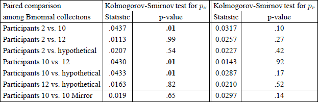
Table 3 provides comparisons of the simulated sampling distributions for p ν and pr among pairs of binomial collections that generated the iid data. For the comparison of the simulated sampling distributions, the Kolmogorov-Smirnov test finds the three pairs differ significantly from each other for p ν. The corresponding test for pr did not yield any significant disagreements among simulated sampling distributions, even though Figure 3 suggests a deviation from uniformity for the sampling distribution for pr on data simulated from the collection of binomials that best fits Participant 10 in Cash I of RDDS. This makes the analysis for pr somewhat more ambiguous.
Table 3: Comparison of simulated sampling distributions for p ν and pr for different collections of binomials.
In each histogram of Figures 2 and 3, the left tail of the distribution is of utmost importance, because it shows how often one will observe small p-values when the null hypothesis holds. This means that the left tail of the histogram gives an idea of Type-I error rates: A spike in the left tail suggests that the Type-I error rate is higher than it should be, because there are too many small p-values. A trough in the left tail suggests a conservative test because there are not enough small p-values to reject the null at a rate of α when we use a significance level of α.
The requirement that a p-value be uniformly distributed under the null hypothesis applies only for continuous statistics. However, the novel statistics underlying p ν and pr can, in fact, only take finitely many different values in data like those in RDDS. Therefore, it may be more informative to compare nominal Type-I error rates (α) with the actual rates of false rejection, for various nominal Type-I error rates when analyzing data sets that we know to be iid. We report this in Table 4. There appears to be little rhyme or reason to the actual Type-I error rates. For p ν, the test appears to be conservative, except for data simulated according to Participant 10’s best fitting binomials. Strangely, though, as we move from Participant 10 to its “mirror,” where we replaced the binomial probabilities of “success” by probabilities of “failure” the testFootnote 6 is no longer conservative, even though these binary choice probabilities are the same and differ only by how pairwise choices are labeled. A test of iid should not depend on whether “a pairwise choice of x over y” is always coded as “a success (for x)” or always coded as “a failure (for y)” in the Bernoulli process and the corresponding Binomials.
Table 4: Nominal versus actual Type-I error rates for Reference BirnbaumBirnbaum’s (2012) tests of iid.
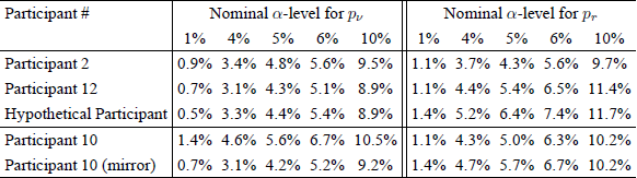
For the test based on pr, even though Figure 3 suggested that four of the five distributions of p-values, in their entirety, do not differ significantly from a uniform distribution, it is rather salient that the Type-I error rates are nonetheless inflated for two of the three cases. Again, the actual Type-I error rate appears to vary quite substantially, depending on the underlying binomial probabilities. This strongly suggests that the results of Birnbaum’s tests do not depend just on whether data are iid or not, they depend on the choice probabilities themselves. They also depend on the way that binary choices are coded. This does not strike us as a desirable property of a meaningful test for iid sampling.
The analyses in this section were based on simulating iid data from given collections of binary choice probabilities. For real data, where we do not know the underlying binary choice probabilities that hold under the null hypothesis, we cannot know the Type-I error rates of Birnbaum’s tests. All in all, in contrast to the Reference Smith and BatchelderSmith and Batchelder (2008) test, which rests on analytically derived expected values and standard errors, and which the RDDS data pass with flying colors, Reference BirnbaumBirnbaum’s (2012) two tests of iid sampling currently lack a solid and coherent mathematical foundation.
5 Do the findings of Reference BirnbaumBirnbaum (2012) replicate within participant?
We now consider whether small values of p ν and/or pr, if they were to serve as a proxy for iid violations, at least have a coherent substantive interpretation. Reference BirnbaumBirnbaum (2012) analyzed only a fraction of RDDS’ data. As we explained in the introduction and illustrated in Table 1, the experiment of Regenwetter et al. (2011) contained three different stimulus sets, labeled Cash I, Cash II, and Noncash, as well as various Distractor items many of which resembled either the Cash or the Noncash items. All stimuli and distractors were mixed with each other within the same experiment (see Table 1). When thinking about iid sampling, we may be concerned about memory effects: The decision maker might recognize previously seen stimuli, recall the choices previously made, and attempt to either be consistent or seek variety. Hence, choices might be interdependent and/or choice probabilities might drift over time because memory of earlier choices might interfere with new choices.
While all Cash I and Cash II stimuli were two-outcome gambles for very similar cash amounts of money, the Noncash gambles involved prizes such as free movie rentals, free coffee, free books, etc. The purpose of the Distractor items and of the intermixing of different stimulus sets was to reduce or eliminate the role of memory in repeated choices from the same stimulus set. Yet, if nonetheless memory affected the choice probabilities or created dependencies, this effect should be most pronounced in the Noncash condition because these stimuli were arguably much more recognizable. Second, the Cash I and Cash II stimuli looked so similar to each other that only a person with knowledge of the experimental design can tell which stimuli belong to which stimulus set.Footnote 7 Since the data collections for Cash I, Cash II, and Noncash gambles were fully interwoven with each other, any substantive conclusions about non-iid responses, if valid in one stimulus set, should replicate in another. We do not know how to make conceptual sense of concluding, say, that a person’s choices on Trials 1, 5, 9, 13, …, 797 were iid, while choices on Trials 4, 8, 12, 16, …, 800 were not iid.
Because of these considerations, we checked whether Reference BirnbaumBirnbaum’s (2012) conclusions about non-iid sampling are consistent across stimulus sets, and whether the alleged violations are indeed more pronounced in the Noncash condition. Hence, we applied Reference BirnbaumBirnbaum’s (2012) R code not only on the Cash I gambles, as was done in Reference BirnbaumBirnbaum (2012), but also on the Cash II and Noncash gambles. The results of our analysis of these three sets are given in Table 5 under the headingFootnote 8 “Full Data Sets”. The R code computes simulated random permutations of the data: We used 10,000 such pseudo-random permutation iterations per analysis. Values of p ν and pr smaller than 0.05 are marked in bold. Values that would round to 0.05 are given to three significant digits. Cases where the linear order model is rejected are in parentheses. Cases that were undefined due to division by zero are marked with a −. We confirm Birnbaum’s finding that, in Cash I, four values of p ν are smaller than 0.05.Footnote 9 In addition, there are six such values in Cash II and four in Noncash. For pr, Reference BirnbaumBirnbaum (2012) reports six values smaller than 0.05 in Cash I, and we find five in each stimulus set. However, it is important to note that not a single individual generated small values of p ν or pr for all three sets.
Table 5: Summary of p ν and pr values, rounded to two significant digits, according to the method of Reference BirnbaumBirnbaum (2012) for Cash I, Cash II, and Noncash of Regenwetter et al. (2011), for both the full data sets, as well as the reduced data sets where the first four trials for each gamble pair pair were dropped.
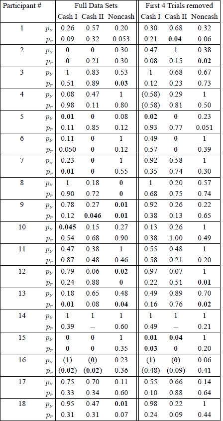
Following the train of thought in Reference BirnbaumBirnbaum (2012), each of these “significant” values might suggest, by itself, that the participant might violate iid sampling. However, the Noncash case has relatively few “violations”, even though this should be the prime source of potential memory effects that could cause interdependencies and/or make the probabilities change in some systematic way. This lack of replicability is consistent with our concern in the previous section, namely that small values of p ν and/or pr may be difficult to interpret. On the other hand, if we give MB the benefit of the doubt and we presume that the tests really do detect violations of iid, then the lack of replications could alternatively be interpreted as indicating very small effect sizes. In that case, the iid assumption might be violated, but only so slightly that it does not turn up significant very often. In that case, the question would arise how the analysis of RDDS would really be affected by an iid assumption that is only an approximation, but a close approximation, of the data.
We have shown that the RDDS data pass Reference Smith and BatchelderSmith and Batchelder’s (2008) test of iid sampling with top marks. We have shown that Reference BirnbaumBirnbaum’s (2012) statistics p ν and pr may not be p-values, that their Type-I error rates are unknown, and that these statistics appear to depend on more than just iid sampling alone, they even appear to depend on how data are coded. We have now established that no single participant, out of 18 participants, has consistently small values of p ν and/or pr across all three stimulus sets, either. Combining these observations, we see no merit in interpreting values of p ν< 0.05 and/or pr < 0.05 as pin-pointing individual participants who violate iid sampling. Likewise, we see no justification for the much broader blanket statement that “the data of Regenwetter, et al. (2011) do not satisfy the iid assumptions required by their method of analysis” (Reference BirnbaumBirnbaum, 2012, p. 99).
6 Could RDDS’s findings be an artifact of warm-up effects?
The discussion around Reference BirnbaumBirnbaum’s (2012) Table 2 suggests that decision makers might change their choice probability after the first few trials. We consider whether the great model fit in RDDS could be an accidental artifact of drifting choice probabilities in the first few trials due to some sort of warm-up period during which the decision makers familiarized themselves with the experiment.
Since Reference BirnbaumBirnbaum (2012) stressed that violations of iid sampling may have led to false acceptance of the linear order model in Regenwetter et al. (2011), we consider whether, by dropping the first four of twenty trials for all gamble pairs, we are able to reject the linear order model on more participants. Starting from Reference BirnbaumBirnbaum’s (2012) Table 2, we dropped the first four trials for each gamble pair, every stimulus set, and every participant. Note that, to decide how many trials to drop, we inspected the data of only the one participant and one stimulus set discussed in Reference BirnbaumBirnbaum’s (2012) Table 2.Footnote 10
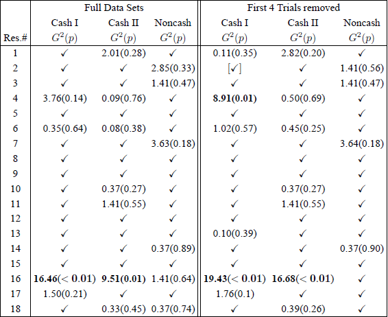
Table 6 shows the results of two analyses of the data in Regenwetter et al. (2011) using a newer software for order-constrained inference.Footnote 11 A checkmark ✓ indicates perfect fit, where the choice proportions fully satisfy the triangle inequalities, hence the model cannot be rejected no matter how small the significance level α. For all cases with choice proportions outside the linear order model, we provide the test statistic G 2 followed by its p-value. G 2 values cannot be compared across cells due to order-constrained inference. Significant violations of the linear order model are marked in bold. One analysis [ marked in brackets ] involved prior inspection of the data. As we drop the first four trials for all stimuli and participants the linear order model fits the data again very well. One person, Participant 16, violates Cash I and Cash II significantly in the full data sets. This person also violates the model in the reduced data. As we move from the full to the reduced data, one nonsignificant violation becomes significant (Participant 4, Cash I), two nonsignificant violations become perfect fits and two perfect fits become nonsignificant violations, giving a nearly identical overall picture of goodness-of-fit. This pattern of results demonstrates clearly that the excellent fit of the model in RDDS was not an artifact of a potential 4-trial-per-gamble-pair warm-up as Reference BirnbaumBirnbaum’s (2012) discussion of his Figure 2 seems to suggest.
Table 6: Analysis of the linear order model on the full data sets and on reduced data sets where the first four trials for each gamble pair are dropped. A checkmark ✓ indicates perfect fit.
7 What do Reference BirnbaumBirnbaum’s (2012) hypothetical data tell us about “true-and-error” models?
Linear orders are a type of transitive preference.Footnote 12 RDDS tested the linear order model as a proxy for testing transitivity of preferences when preferences are allowed to vary between and within persons. Reference BirnbaumBirnbaum (2012) provided three tables of hypothetical data to suggest that one can construct thought experiments in which the approach of RDDS will classify all three data sets as transitive when Birnbaum generated some of the hypothetical data by simulating certain intransitive decision makers. Reference BirnbaumBirnbaum (2012) suggested that “true-and-error” models overcome this challenge. We will now explain briefly how a “true-and-error” model works and then prove that such models do not overcome the stated challenge.
Consider once again Table 1 with the first 36 trials in the RDDS experiment. The basic unit of analysis in RDDS is the binary response on one trial. In contrast, the basic unit of analysis and the basic theoretical primitive in “true-and-error” models is that of a “response pattern”. Consider the Cash II gamble set. Because Cash II involved five distinct lotteries and all possible pairs of these five gambles, there are 10 distinct pairs of gambles in Cash II, each of which was presented 20 times. Each of Trials 4, 8, 12, 16, 20, 24, 28, and 32 is the “first replicate” of a gamble pair in Cash II, whereas Trial 36 is the “second replicate” of the lottery pair used previously in Trial 4. In a “true-and-error” model, the pattern of responses in Trials 4, 8, 12, 16, 20, 24, 28, 32 (and two more later trials), namely RRRLRLRR…, form one observation, namely the observed choice pattern for the first replicate (see the underlined responses in the last column of Table 1). The second replicate overlaps with the first in time in that Trial 36 is already part of the observed pattern for the second replicate. We call blocking assumption the assumption that pairwise choices in Trials 4, 8, 12, 16, 20, 24, 28, 32, and two more later trials can be blocked together to form a single observation RRRLRLRR… of one pattern. According to the blocking assumption, the pairwise choice in Trial 36 is not interchangeable with the choice in Trial 4, because Trial 36 is part of the second “replicate”. In Table 1 the respondent happens to have chosen R again as in Trial 4, but if this observed choice were L, the blocking assumption would disallow exchanging the observations in Trials 4 and 36.
In the analysis of RDDS, the 200 trials that make up the data for a given stimulus set (say, Cash II) are treated as 20 observations for each of 10 binomials (this gives the usual 20 observations per binomial that is recommended as a rule of thumb for using asymptotic statistics). In a “true and error model” the same 200 binary choices form 20 observations (20 observed patterns from 20 replicates) of one single multinomial with 210 = 1,024 cells, i.e., with 1,023 degrees of freedom. This is because there are 1,024 distinct possible patterns of 10 binary choices. For a multinomial with over 1,000 degrees of freedom, 20 observations can be labeled extremely sparse data that are nowhere close to warranting the use of asymptotic distributions for test statistics.
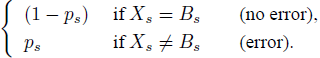
We now introduce what we will label the standard true-and-error model [henceforth STE] for such a multinomial. The STE model spells out how a binary response pattern, the primitive unit of observation for the model, is related to individual binary responses on individual trials. In the STE model the decision maker has a single, deterministic, fixed, “true” preference pattern throughout the experiment, and the reason that he or she does not choose consistently with that preference pattern is because she or he makes errors (trembles) with some probability. According to Reference BirnbaumBirnbaum (2004, pp. 59, 61), Reference BirnbaumBirnbaum (2007, p. 163), Reference Birnbaum and BahraBirnbaum and Bahra (2007, p. 1024), Reference Birnbaum and GutierrezBirnbaum and Gutierrez (2007, p. 100), Reference BirnbaumBirnbaum (2008a, p. 483), Reference BirnbaumBirnbaum (2008b, p. 315), Reference Birnbaum and LaCroixBirnbaum and Lacroix (2008, p. 125), Reference Birnbaum and SchmidtBirnbaum and Schmidt (2008, p. 82), Reference BirnbaumBirnbaum (2010, p. 369), as well as Reference Birnbaum and SchmidtBirnbaum and Schmidt (2010, p. 604), errors occur independently of each other, with the error probability of each gamble pair being constant over time. Denoting the decision maker’s true preference pattern as B and letting Bs denote the entry in B for gamble pair s, i.e., the person’s true preference for gamble pair s, and denoting by ps the probability of making an error when responding to gamble pair s, the probability that this decision maker gives response Xs at time t does not depend on t and it equals
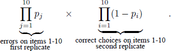
For example, suppose that there are 10 pairs of gambles. Following the equations in the referenced papers, the probability of a binary pattern in which a given decision maker chooses correctly on Gamble Pairs 6, 7, and 10 and chooses incorrectly on Gamble Pairs 1, 2, 3, 4, 5, 8, 9, according to the STE model, is
There are 1,024 such formulae to provide the probabilities of all 1,024 different choice patterns that are possible in the STE model. In Table 1 we used labels L and R to refer to left-hand-side and right-hand-side gambles. Instead, we could also label one gamble as Gamble 0 and the other gamble as Gamble 1 (and in the process drop the distinction of the side on which a given gamble was presented visually), and then record, for each trial a zero or a one to code which gamble was chosen. If we fix the sequence by which we consider the gamble pairs in such a binary codingFootnote 13, we can represent both the “true” preference and each of the observed preference patterns as 10-digit strings of zeros and ones.
Say, if the decision maker’s true preference is binary pattern 0000000000
then, by Formula 6, the observed
pattern 1111100110 has probability ![]() . The STE model also spells out what
happens if each question (gamble pair) is presented on two replicates. If the
decision maker makes 10 choices on 10 distinct gamble pairs in one replicate, and
another set of 10 choices on the same 10 gamble pairs in a second replicate, the
probability that s/he makes 10 errors on the first replicate and makes no errors on
the second replicate, according to STE is,
. The STE model also spells out what
happens if each question (gamble pair) is presented on two replicates. If the
decision maker makes 10 choices on 10 distinct gamble pairs in one replicate, and
another set of 10 choices on the same 10 gamble pairs in a second replicate, the
probability that s/he makes 10 errors on the first replicate and makes no errors on
the second replicate, according to STE is,
We now move to the hypothetical data in Reference BirnbaumBirnbaum (2012). Reference BirnbaumBirnbaum (2012) argued that the linear order model analysis of RDDS may fail to distinguish transitive from intransitive cases when iid is violated. For convenience, we reproduce the hypothetical data in question in Table 7. The columns list hypothetical gamble pairs, the rows list the hypothetical replicates (repetitions). In the interior of the table an entry “1” indicates the choice of the first gamble in the gamble pair, and a “0” indicates a choice of the second gamble in a gamble pair.
Table 7: Hypothetical data in Reference BirnbaumBirnbaum’s (2012) Tables A.4 (top), A.5. (center), and A.6. (bottom). A “1” indicates choice of the first option in pair, a “0” indicates choice of the second option. For each column of data, we also provide the result of a test for iid sampling of Reference Smith and BatchelderSmith and Batchelder (2008, p.727) using confidence intervals of point estimates ± 2 standard errors (or ± 1.96 standard errors. The results of using 1.96 or 2 standard errors matched throughout.).
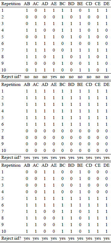
Our table also gives the results of the iid test of Reference Smith and BatchelderSmith and Batchelder (2008). For the top data set, there are 10 separate tests, of which one turns out significant. Reference BirnbaumBirnbaum (2012) states that these data were iid generated, hence we have one Type I error by Reference Smith and BatchelderSmith and Batchelder’s (2008) test in ten tests. (Recall that our analysis in Table 2 yielded significant results in 3% of cases in RDDS.) In the data in the center of Table 7, all columns are the same, hence we only need to apply Smith and Batchelder’s test once. Indeed, it is significant, consistent with a violation of iid sampling. In the third data set, which involves only two types of column collections, the corresponding two tests of Reference Smith and BatchelderSmith and Batchelder (2008) turn out significant both times, consistent with a violation of iid sampling. Reference BirnbaumBirnbaum’s (2012) latter two hypothetical data sets are quite different from RDDS’ real data.
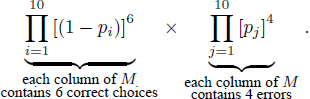
Reference BirnbaumBirnbaum (2012) stated that the RDDS analysis, by counting pairwise choice proportions only, treat the three tables the same and classify all three cases as transitive, whereas true-and error models would distinguish the first, transitive, case from the other two, intransitive, cases. We first show that standard true-and-error models (as used in Reference BirnbaumBirnbaum 2004, pp. 59, 61; Reference Birnbaum and GutierrezBirnbaum, 2007, p. 163; Reference Birnbaum and BahraBirnbaum & Bahra, 2007, p. 1024; Reference Birnbaum and GutierrezBirnbaum & Gutierrez, 2007, p. 100; Reference BirnbaumBirnbaum, 2008a, p. 483; Reference BirnbaumBirnbaum, 2008b, p. 315; Reference Birnbaum and LaCroixBirnbaum and Lacroix, 2008, p. 125; Reference Birnbaum and SchmidtBirnbaum & Schmidt, 2008, p. 82; Reference Birnbaum and SchmidtBirnbaum, 2010, p. 369; Reference Birnbaum and SchmidtBirnbaum & Schmidt, 2010, p. 604), will also treat all three tables the same and will likewise classify all three data tables as transitive. For each of Tables A.4-A.6 in Reference BirnbaumBirnbaum (2012), we can expand the formulations of the STE model in Formulae 5 and 7 to a situation with 10 replicates. The probability of the observations in each table is given by
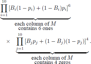
For example, if the true preference is B = 1111111111, the probability of the data in each table is given by
If, as is usually the case, we restrict the error probabilities to be ps < 0.5, ∀s, then the maximum likelihood estimate will yield the “true” preference pattern 1111111111 and estimated error probabilities of 0.4 for every error term, in every one of the three Tables A.4-A.6 of Reference BirnbaumBirnbaum (2012), as summarized in our Table 7. The STE model analysis cannot distinguish the three hypothetical data tables. Reference BirnbaumBirnbaum (2012) designed these three hypothetical data sets to illustrate alleged weaknesses of the analysis of RDDS and strengths of the “true-and-error” approach. Yet, like the analysis used in RDDS, the STE model analysis cannot differentiate between the data in the three tables either, and it will also classify all three cases as transitive.
In the discussion of Tables A.4-A.6, Reference BirnbaumBirnbaum (2012, p. 106) states that Reference Birnbaum and BahraBirnbaum and Bahra (2007) “found that some people had 20 responses out of 20 choice problems exactly the opposite between two blocks of trials. Such extreme cases of perfect reversal mean that iid is not tenable because they are so improbable given the assumption of iid.” If true, then this would mean that Reference Birnbaum and BahraBirnbaum and Bahra’s (2007) analysis, which used a STE model with iid errors (Reference Birnbaum and BahraBirnbaum and Bahra, 2007, p. 1024), is itself “not tenable” on those data, in Birnbaum’s words.
We have shown that the STE model, the model used in 10 or more published papers, cannot distinguish between the three data tables any better than the analysis in RDDS. We have also shown in Table 7 that Reference Smith and BatchelderSmith and Batchelder’s (2008) test successfully picks up the iid violations that Birnbaum built into two of the tables. Recall that this is the test that the RDDS data passed with flying colors.
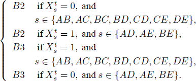
Next, consider a modification of the STE model test in which there is still a single true preference, but where the iid assumption for errors is dropped. Then the data in Reference BirnbaumBirnbaum’s (2012) Table A.5 (center of our Table 7) can originate from a person with transitive true preference pattern 1111111111 who makes no errors for the first 60 binary choice trials (i.e., the first 6 lines in the table) and who makes errors for all remaining trials of the study. However, this person can instead have fixed intransitive true preference pattern 0011001000 and generate the same data because she or he makes no errors on the first 6 trials of stimuli AD,AE,BE but errors in all first 6 trials of stimuli AB,AC,BC,BD,CD,CE,DE, then switches to the opposite error behavior for the remaining four replicates. Similar constructions are possible for Reference BirnbaumBirnbaum’s (2012) Tables A.4 and A.6 (top and bottom of our Table 7). If errors are allowed to be interdependent and if error probabilities are allowed to change over the course of the experiment, then “true-and-error” models can generate a perfect fit to any data, no matter what fixed “true preference” they use. In other words, “true-and-error” models without iid assumption for errors are neither identifiable nor testable. They are vacuous, even if they permit only one single and fixed “true” preference.
Finally, we consider what happens in Tables A.4-A.6 (our Table 7) if we consider “true-and-error” models in which the preferences are allowed to vary. For example, a person may have preference pattern B1 = 1111111111, say, 60% of the time, and preference pattern B0 = 0000000000 on 40% of occasions. We denote this as Hypothesis H. Or the person may have preference state B2 = 0011001000, say, 60% of the time, and B3 = 1100110111 the other 40% of the time. We denote this as Hypothesis HH.
Write ![]() for the decision maker’s observed choice for gamble pair s
at replicate t, that is,
for the decision maker’s observed choice for gamble pair s
at replicate t, that is, ![]() is the entry in a given table in
column s and row t. Assume for a moment, that
there are no errors, i.e., ps = 0, for
s ∈ {AB, AC,
AD, AE, BC,
BD, BE, CD,
CE, DE}. We obtain a perfect fit for the data
in each of Tables A.4–A.6 in Reference BirnbaumBirnbaum
(2012) under Hypothesis H by assuming that the decision maker is in state
B1 whenever he or she gives an answer
is the entry in a given table in
column s and row t. Assume for a moment, that
there are no errors, i.e., ps = 0, for
s ∈ {AB, AC,
AD, AE, BC,
BD, BE, CD,
CE, DE}. We obtain a perfect fit for the data
in each of Tables A.4–A.6 in Reference BirnbaumBirnbaum
(2012) under Hypothesis H by assuming that the decision maker is in state
B1 whenever he or she gives an answer ![]() in the Table,
and that the decision maker is in state B0 whenever he or she gives
an answer
in the Table,
and that the decision maker is in state B0 whenever he or she gives
an answer ![]() in the Table. Likewise, we obtain a
perfect fit of the data in each of Tables A.4-A.6 in Reference BirnbaumBirnbaum (2012) by assuming that the decision maker is in state
in the Table. Likewise, we obtain a
perfect fit of the data in each of Tables A.4-A.6 in Reference BirnbaumBirnbaum (2012) by assuming that the decision maker is in state
In a “true-and-error”model test where preference patterns may vary at any time, both Hypothesis H and Hypothesis HH will fit the data in all three tables perfectly even when setting all error probabilities to zero. The “true-and-error” model with variable preferences is unidentifiable and can generate a perfect fit to any data whatsoever, such as those in Tables A.4-A.6 in Reference BirnbaumBirnbaum (2012). Like the previous case, this “true-and-error” model is vacuous.
Combining the last two points, if “true preferences” can vary at any time, if the error probabilities are positive, if these error probabilities are allowed to change at any time, and if errors are allowed to be interdependent, the unidentifiability and nontestability problem is further exacerbated and multiple mutually exclusive “true-and-error” models will vacuously and simultaneously fit any data perfectly.
How does MB propose to render tests of “true-and-error” models non-vacuous? First, accommodating non-iid errors seems challenging.Footnote 14 Second, MB uses a “blocking” assumption, not needed by RDDS, which regulates, at the researcher’s discretion, when exactly preferences are permitted to change. Under the “blocking” assumption, preferences are fixed during replicates and preferences are permitted to change from one replicate to the next. In other words, the decision maker must keep or may change their preference at arbitrarily determined time points that are selected by the scholar but not communicated to the participant. Considering Table 1, the blocking assumption for a “true-and-error” model with variable preferences from one block to the next assumes that the decision maker stays in the first true preference for the first replicate of those two gamble pairs that were not yet presented in the first 36 trials, whereas the decision maker is allowed to have already moved to a new preference state for the second replicate as of Trial 36 where we observe the second replicate of the lottery pair “36% chance of $24.44” versus “28% chance of $31.43”. It is the “blocking” assumption that allows Reference BirnbaumBirnbaum (2012) to gather data into tables like Tables A.4-A.6 where each row is interpreted as one fixed preference state. Our example above has shown that in the absence of the “blocking” assumption both Hypotheses H and HH can simultaneously fit all the data in the three tables perfectly, even though they are mutually incompatible, hence the model becomes vacuous and uninformative. The sequence of trials in RDDS in Table 1, where the second replicate starts on Trial 36 (for some gamble pairs) before the first replicate has even been completed (for some other gamble pairs), shows how implausible it is to assume that a decision maker switches preferences between, but not within, blocks of trials that form a replicate. The decision maker has no way of knowing when she or he may use the first preference state and when she or he may use the second preference state. Similar concerns apply also when replicates are fully separated in time and do not overlap.
8 Conclusion.
Every researcher depends on some simplifying assumptions. The state-of-the-art “order-constrained likelihood-ratio” test in RDDS is currently available only under the auxiliary assumption of iid data. Our application of Reference Smith and BatchelderSmith and Batchelder’s (2008) test suggests that RDDS’ data, indeed, satisfy that iid assumption. Reference BirnbaumBirnbaum’s (2012) inference that the RDDS data violate iid rests on questionable mathematical conjectures and leads to incoherent interpretations within participants. In particular, Birnbaum’s proposed test statistics have unknown Type-I error rates that are sometimes larger, sometimes smaller than the nominal α-level, even for the same data, depending on how responses are coded.
Reducing 200 observations for a given stimulus set to a manageable set of statistics that can serve as point estimates of parameters and ultimately help test theories, requires making one assumption or another. We have shown that Birnbaum’s proposed alternative rests on its own, highly restrictive assumptions, some of which, to date, have not been tested. Not only are the errors routinely assumed to be iid, the analysis also fundamentally depends on the “blocking” assumptions according to which pairwise choices at certain time points, such as Trials 4, 8, 12, 16, 20, 24, 28, 32, and two more trials after Trial 36 in RDDS (see Table 1) form one observation, whereas another collection of trials (starting with Trial 36 in Table 1) form another observation. Using Reference BirnbaumBirnbaum’s (2012) hypothetical data, we have illustrated how dropping these assumptions would make the “true-and-error” models vacuous and uninformative. A companion paper has shown that, while many classical probabilistic choice models, such as Reference LuceLuce’s (1959) choice model, the weak utility model (Reference Becker, DeGroot and MarschakBecker et al.,1963; Reference Block, Marschak, Olkin, Ghurye, Hoeffding, Madow and MannBlock & Marschak, 1960; Reference Luce, Suppes, Luce, Bush and GalanterLuce & Suppes, 1965; Reference Marschak, Arrow, Karlin and SuppesMarschak, 1960), and the most heavily used “true-and-error” model in the literature (Reference BirnbaumBirnbaum (2004, 2007, 2008a,b, 2010; Reference Birnbaum and BahraBirnbaum & Bahra, 2007; Reference Birnbaum and GutierrezBirnbaum & Gutierrez, 2007; Reference Birnbaum and LaCroixBirnbaum & Lacroix, 2008; Reference Birnbaum and SchmidtBirnbaum & Schmidt, 2008, 2010), require a person to have a single fixed preference throughout an entire experiment, the model in RDDS not only allows preferences to be probabilistic, it even has the somewhat unique property that one can average different probability distributions satisfying the model, and still satisfy the model. Not only does the model in RDDS stand out in its ability to model variability of preferences, it even allows that variability itself to be non-stationary.
We have shown that MB’s inference of iid violations in the RDDS data are premature: The RDDS data do not appear to violate iid sampling. We have also provided some documentation on Reference BirnbaumBirnbaum’s own (2012) hypothetical data, suggesting the opposite of Reference BirnbaumBirnbaum’s (2012) conclusion: “True-and-error” models hinge far more strongly on their assumptions than does the analysis in RDDS.
Appendix.
Expected value and standard error of Ai in Eq. 21 of Reference Smith and BatchelderSmith and Batchelder (2008, p. 727).
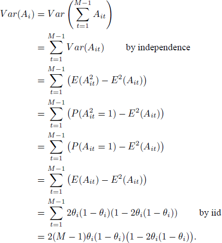
Writing M for the number of repetitions, let
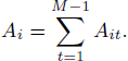
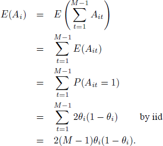
First, we first show that the expected value of Ai is
![]() when iid holds.
when iid holds.
Second, we show that, when iid holds, the standard error of Ai equals


 Open access