1 Introduction
In non-axisymmetric equilibria, confinement of guiding-centre orbits is not guaranteed, and enhanced neoclassical losses occur at low collisionality (Galeev et al. Reference Galeev, Sagdeev, Furth and Rosenbluth1969; Connor & Hastie Reference Connor and Hastie1974; Nemov et al. Reference Nemov, Kasilov, Kernbichler and Heyn1999). Significant optimization efforts are used to reduce neoclassical losses to acceptable levels (Mynick Reference Mynick2006, and references therein). However, even with good optimization for thermal particle confinement, energetic losses, such as those from alpha particles in stellarator fusion reactors, can be high. Calculations showed that when scaled to a reactor, both the quasihelically symmetric experiment HSX and the quasiaxisymmetric configuration NCSX had a loss of most magnetically trapped alpha particles within a thermalization time (Mynick, Boozer & Ku Reference Mynick, Boozer and Ku2006; Nemov, Kasilov & Kernbichler Reference Nemov, Kasilov and Kernbichler2014). In this paper, we look at optimizations specifically targeting energetic particle losses in stellarator equilibria and show that it is possible to generate quasihelically symmetric configurations at the ARIES-CS scale (Najmabadi et al. Reference Najmabadi, Raffray, Abdel-Khalik, Bromberg, Crosatti, El-Guebaly, Garabedian, Grossman, Henderson and Ibrahim2008) which reduce energetic particle losses within the mid-radius to below 1 %.
Energetic particle confinement has long been thought of as a weak point for stellarators. For example, a simple scaling of the NCSX configuration, a quasiaxisymmetric configuration, to a reactor scale equilibrium (
 $450~\text{m}^{3}$
volume at 5.7 T) produced a configuration which lost 27 % of alpha particles promptly, nearly equivalent to the trapped particle fraction (Mynick et al.
Reference Mynick, Boozer and Ku2006). Prompt losses of this magnitude negatively affect the energy balance and impact ignition requirements. Further optimization of the equilibrium reduced alpha particle energy losses to
$450~\text{m}^{3}$
volume at 5.7 T) produced a configuration which lost 27 % of alpha particles promptly, nearly equivalent to the trapped particle fraction (Mynick et al.
Reference Mynick, Boozer and Ku2006). Prompt losses of this magnitude negatively affect the energy balance and impact ignition requirements. Further optimization of the equilibrium reduced alpha particle energy losses to
 ${\sim}5\,\%$
. However, this level of alpha particle loss was still large enough that the resulting heat flux from alpha particles alone exceeded engineering limits on the divertor plates (Mau et al.
Reference Mau, Kaiser, Grossman, Raffray, Wang, Lyon, Maingi, Ku and Zarnstorff2008). These calculations did not include the effects arising from finite coils. Finite coils can give rise to components of the magnetic field spectrum in which the toroidal mode number is a integer multiple of the number of coils. These high-order magnetic field spectral modes can be deleterious to energetic particle confinement. Coil-ripple modes also appear in tokamaks and can produce energetic particle losses. Tokamaks such as ITER include ferritic inserts to reduce energetic particle losses from coil ripple (Tobita et al.
Reference Tobita, Nakayama, Konovalov and Sato2003).
${\sim}5\,\%$
. However, this level of alpha particle loss was still large enough that the resulting heat flux from alpha particles alone exceeded engineering limits on the divertor plates (Mau et al.
Reference Mau, Kaiser, Grossman, Raffray, Wang, Lyon, Maingi, Ku and Zarnstorff2008). These calculations did not include the effects arising from finite coils. Finite coils can give rise to components of the magnetic field spectrum in which the toroidal mode number is a integer multiple of the number of coils. These high-order magnetic field spectral modes can be deleterious to energetic particle confinement. Coil-ripple modes also appear in tokamaks and can produce energetic particle losses. Tokamaks such as ITER include ferritic inserts to reduce energetic particle losses from coil ripple (Tobita et al.
Reference Tobita, Nakayama, Konovalov and Sato2003).
Recent optimizations of a quasiaxisymmetric equilibrium with volume
 $1900~\text{m}^{3}$
and magnetic field on axis of 5 T by Henneberg et al. (Reference Henneberg, Drevlak, Nührenberg, Beidler, Turkin, Loizu and Helander2019) show losses at normalized toroidal flux
$1900~\text{m}^{3}$
and magnetic field on axis of 5 T by Henneberg et al. (Reference Henneberg, Drevlak, Nührenberg, Beidler, Turkin, Loizu and Helander2019) show losses at normalized toroidal flux
 $s=\unicode[STIX]{x1D713}/\unicode[STIX]{x1D713}_{a}=0.25$
of
$s=\unicode[STIX]{x1D713}/\unicode[STIX]{x1D713}_{a}=0.25$
of
 ${\approx}5\,\%$
after 100 ms, when collisions and an electric field are included in the simulation. Here,
${\approx}5\,\%$
after 100 ms, when collisions and an electric field are included in the simulation. Here,
 $\unicode[STIX]{x1D713}_{a}$
represents the toroidal flux at the edge. The normalized flux
$\unicode[STIX]{x1D713}_{a}$
represents the toroidal flux at the edge. The normalized flux
 $s$
will be used throughout the paper.
$s$
will be used throughout the paper.
In contrast to quasiaxisymmetric equilibria, energetic particle calculations performed by Lotz showed that quasihelically symmetric equilibria could provide improved alpha particle confinement (Lotz et al.
Reference Lotz, Merkel, Nuhrenberg and Strumberger1992). Lotz calculated that collisionless alpha particle losses for a quasihelically symmetric (QHS) equilibria with volume
 $727~\text{m}^{3}$
and magnetic field of 5 T were 3 % after 200 ms for
$727~\text{m}^{3}$
and magnetic field of 5 T were 3 % after 200 ms for
 $s\approx 0.2$
. Lotz also showed that for configurations optimized to eliminate bootstrap current, finite plasma pressure improves confinement. In examining a HELIAS configuration, a reactor scale device based on an early design of W7-X, Lotz found core alpha particle losses were reduced to 10 % at normalized pressure,
$s\approx 0.2$
. Lotz also showed that for configurations optimized to eliminate bootstrap current, finite plasma pressure improves confinement. In examining a HELIAS configuration, a reactor scale device based on an early design of W7-X, Lotz found core alpha particle losses were reduced to 10 % at normalized pressure,
 $\unicode[STIX]{x1D6FD}=2\unicode[STIX]{x1D707}_{0}P/B^{2}=0.05$
from losses of
$\unicode[STIX]{x1D6FD}=2\unicode[STIX]{x1D707}_{0}P/B^{2}=0.05$
from losses of
 ${\approx}30\,\%$
at
${\approx}30\,\%$
at
 $\unicode[STIX]{x1D6FD}=0.0$
. In the above expression for
$\unicode[STIX]{x1D6FD}=0.0$
. In the above expression for
 $\unicode[STIX]{x1D6FD}$
,
$\unicode[STIX]{x1D6FD}$
,
 $P$
is the plasma pressure and
$P$
is the plasma pressure and
 $B$
is the magnetic field strength.
$B$
is the magnetic field strength.
More detailed calculations of energetic particle losses were also performed for 60 keV protons in W7-X by Drevlak et al. (Reference Drevlak, Geiger, Helander and Turkin2014). These protons have equivalent normalized gyroradius,
 $\unicode[STIX]{x1D70C}^{\ast }=\unicode[STIX]{x1D70C}/a$
, the ratio of the ion gyroradius to the minor radius, as alpha particles in a device with volume
$\unicode[STIX]{x1D70C}^{\ast }=\unicode[STIX]{x1D70C}/a$
, the ratio of the ion gyroradius to the minor radius, as alpha particles in a device with volume
 $1800~\text{m}^{3}$
and magnetic field on axis of 5 T. It was seen that even in the most optimized configurations of W7-X presented by Drevlak et al., prompt losses at the mid-radius exceeded 10 %. Importantly, these calculations did include the actual magnetic fields produced from coils rather than idealized equilibria.
$1800~\text{m}^{3}$
and magnetic field on axis of 5 T. It was seen that even in the most optimized configurations of W7-X presented by Drevlak et al., prompt losses at the mid-radius exceeded 10 %. Importantly, these calculations did include the actual magnetic fields produced from coils rather than idealized equilibria.
Losses of energetic particles in non-axisymmetric equilibria come from two sources. The first source is those from the configuration itself as defined by fixed boundary magnetohydrodynamic equilibrium solutions. Generally, any three-dimensional configuration will have particles with non-zero bounce-averaged radial drift. Perfectly axisymmetric configurations are guaranteed to have no direct collisionless orbit losses. However, in all experiments and prototype reactor designs, finite coils are necessary to generate the magnetic field. These coils break axisymmetry in tokamak configurations by providing ‘coil ripple’. Particles can be trapped within local magnetic wells and then subsequently drift radially out of the plasma and escape. In stellarators finite coils will always produce some error by not matching the target boundary exactly. These errors can produce unwanted terms in the magnetic spectrum, including a coil-ripple term. As in tokamaks, coil ripple in stellarators causes losses due to particles trapped within localized wells. Additionally in stellarators, finite coils can lead to longer wavelength modes in the magnetic spectrum degrading confinement mainly for thermal particles. In this paper, we focus mainly on eliminating the losses from the idealized configuration alone without considering additional losses from finite coils.
The layout of the paper is as follows. In § 2, we discuss the methods we use to optimize stellarator equilibria in general, including a brief introduction to the ROSE code used in this optimization study. Section 3 describes metrics used for optimization of energetic particles in the past, and describes the
 $\unicode[STIX]{x1D6E4}_{c}$
metric that was used to generate the equilibria presented in this paper. Section 4 shows various optimized quasihelically symmetric equilibria that demonstrate excellent confinement of energetic particles, including configurations at different aspect ratios. Finally, § 5 summarizes the results and looks towards the future of energetic particle optimization.
$\unicode[STIX]{x1D6E4}_{c}$
metric that was used to generate the equilibria presented in this paper. Section 4 shows various optimized quasihelically symmetric equilibria that demonstrate excellent confinement of energetic particles, including configurations at different aspect ratios. Finally, § 5 summarizes the results and looks towards the future of energetic particle optimization.
2 Stellarator optimization
Numerous approaches have been developed to reduce neoclassical losses in stellarators (Mynick Reference Mynick2006). One commonly used metric for achieving good neoclassical transport is the effective ripple,
 $\unicode[STIX]{x1D716}_{\text{eff}}$
, introduced by Nemov in Nemov et al. (Reference Nemov, Kasilov, Kernbichler and Heyn1999). This metric can be calculated directly from VMEC equilibria or from field line following and is the geometric component of the diffusion coefficients in the
$\unicode[STIX]{x1D716}_{\text{eff}}$
, introduced by Nemov in Nemov et al. (Reference Nemov, Kasilov, Kernbichler and Heyn1999). This metric can be calculated directly from VMEC equilibria or from field line following and is the geometric component of the diffusion coefficients in the
 $1/\unicode[STIX]{x1D708}$
regime, in which the transport increases with decreasing collisionality. In this regime, the perpendicular diffusion,
$1/\unicode[STIX]{x1D708}$
regime, in which the transport increases with decreasing collisionality. In this regime, the perpendicular diffusion,
 $D_{\bot }\sim \unicode[STIX]{x1D716}_{\text{eff}}^{3/2}v_{dr}^{2}/\unicode[STIX]{x1D708}$
, where
$D_{\bot }\sim \unicode[STIX]{x1D716}_{\text{eff}}^{3/2}v_{dr}^{2}/\unicode[STIX]{x1D708}$
, where
 $v_{dr}$
is the radial drift velocity and
$v_{dr}$
is the radial drift velocity and
 $\unicode[STIX]{x1D708}$
is the collision frequency. The collision frequency in this regime is restricted so that it is greater than the poloidal precession frequency due to
$\unicode[STIX]{x1D708}$
is the collision frequency. The collision frequency in this regime is restricted so that it is greater than the poloidal precession frequency due to
 $\unicode[STIX]{x1D735}B$
and
$\unicode[STIX]{x1D735}B$
and
 $E\times B$
drifts and less than the bounce frequency of a particle trapped in a local magnetic well. As the radial electric field and the corresponding precession frequency increases, a trapped particle can quickly exit from the
$E\times B$
drifts and less than the bounce frequency of a particle trapped in a local magnetic well. As the radial electric field and the corresponding precession frequency increases, a trapped particle can quickly exit from the
 $1/\unicode[STIX]{x1D708}$
regime. Nevertheless, the effective ripple is often used as a means of comparing neoclassical transport between various configurations, as seen for example in figure 15 of Spong (Reference Spong2015).
$1/\unicode[STIX]{x1D708}$
regime. Nevertheless, the effective ripple is often used as a means of comparing neoclassical transport between various configurations, as seen for example in figure 15 of Spong (Reference Spong2015).
A specific subclass of optimized equilibria, quasisymmetric configurations have tokamak-like neoclassical transport provided there is symmetry in the magnetic field strength. In perfect quasisymmetry there are no particles with net radial drifts and hence no
 $1/\unicode[STIX]{x1D708}$
neoclassical transport. Designs of quasisymmetric equilibria were generated by Nührenberg & Zille (Reference Nührenberg and Zille1988). In practice exact quasisymmetry cannot be attained globally in a stellarator (Garren & Boozer Reference Garren and Boozer1991). However, stellarator designs that approximate quasisymmetry generally have favourable neoclassical transport. To date, only one quasisymmetric stellarator has been built and operated, the quasihelically symmetric experiment (HSX) in the University of Wisconsin-Madison (Anderson et al.
Reference Anderson, Almagri, Anderson, Matthews, Talmadge and Shohet1995). However, many other quasisymmetric configurations have been examined including NCSX (Zarnstorff et al.
Reference Zarnstorff, Berry, Brooks, Fredrickson, Fu, Hirshman, Hudson, Ku, Lazarus and Mikkelsen2001), ARIES-CS (Najmabadi et al.
Reference Najmabadi, Raffray, Abdel-Khalik, Bromberg, Crosatti, El-Guebaly, Garabedian, Grossman, Henderson and Ibrahim2008), CHS-QA (Okamura et al.
Reference Okamura, Matsuoka, Nishimura, Isobe, Nomura, Suzuki, Shimizu, Murakami, Nakajima and Yokoyama2001) and a more recent adaptation (Liu et al.
Reference Liu, Shimizu, Isobe, Okamura, Nishimura, Suzuki, Xu, Zhang, Liu and Huang2018) and also by Henneberg et al. (Reference Henneberg, Drevlak, Nührenberg, Beidler, Turkin, Loizu and Helander2019).
$1/\unicode[STIX]{x1D708}$
neoclassical transport. Designs of quasisymmetric equilibria were generated by Nührenberg & Zille (Reference Nührenberg and Zille1988). In practice exact quasisymmetry cannot be attained globally in a stellarator (Garren & Boozer Reference Garren and Boozer1991). However, stellarator designs that approximate quasisymmetry generally have favourable neoclassical transport. To date, only one quasisymmetric stellarator has been built and operated, the quasihelically symmetric experiment (HSX) in the University of Wisconsin-Madison (Anderson et al.
Reference Anderson, Almagri, Anderson, Matthews, Talmadge and Shohet1995). However, many other quasisymmetric configurations have been examined including NCSX (Zarnstorff et al.
Reference Zarnstorff, Berry, Brooks, Fredrickson, Fu, Hirshman, Hudson, Ku, Lazarus and Mikkelsen2001), ARIES-CS (Najmabadi et al.
Reference Najmabadi, Raffray, Abdel-Khalik, Bromberg, Crosatti, El-Guebaly, Garabedian, Grossman, Henderson and Ibrahim2008), CHS-QA (Okamura et al.
Reference Okamura, Matsuoka, Nishimura, Isobe, Nomura, Suzuki, Shimizu, Murakami, Nakajima and Yokoyama2001) and a more recent adaptation (Liu et al.
Reference Liu, Shimizu, Isobe, Okamura, Nishimura, Suzuki, Xu, Zhang, Liu and Huang2018) and also by Henneberg et al. (Reference Henneberg, Drevlak, Nührenberg, Beidler, Turkin, Loizu and Helander2019).
Besides HSX, the only other operating neoclassically optimized stellarator is the quasi-omnigenous W7-X stellarator in Germany (Klinger et al. Reference Klinger, Alonso, Bozhenkov, Burhenn, Dinklage, Fuchert, Geiger, Grulke, Langenberg and Hirsch2016). W7-X was designed as a quasi-omnigenous device and did not target quasisymmetry. Instead, the design targeted a number of physics properties including reduced Pfirsch–Schlüter and bootstrap currents consistent with reduced neoclassical transport.
2.1 Boundary optimization
Finding equilibria that possess good neoclassical transport, whether through quasisymmetry or other optimizations is not trivial. While various schemes are being pursued such as an analytic construction from first principles (Landreman & Sengupta Reference Landreman and Sengupta2018), the conventional method, and the one used to design HSX, W7-X, and NCSX, is to couple a nonlinear boundary optimization with an equilibrium solver. In this optimization scheme, the plasma boundary is parametrized in Fourier modes, such that,
 $$\begin{eqnarray}\displaystyle & \displaystyle R=\mathop{\sum }_{m,n}R_{m,n}^{c}\cos (m\unicode[STIX]{x1D703}-n\unicode[STIX]{x1D701})+R_{m,n}^{s}\sin (m\unicode[STIX]{x1D703}-n\unicode[STIX]{x1D701}) & \displaystyle\end{eqnarray}$$
 $$\begin{eqnarray}\displaystyle & \displaystyle Z=\mathop{\sum }_{m,n}Z_{m,n}^{c}\cos (m\unicode[STIX]{x1D703}-n\unicode[STIX]{x1D701})+Z_{m,n}^{s}\sin (m\unicode[STIX]{x1D703}-n\unicode[STIX]{x1D701}). & \displaystyle\end{eqnarray}$$
Here
 $m$
is a poloidal mode number,
$m$
is a poloidal mode number,
 $n$
is a toroidal mode number,
$n$
is a toroidal mode number,
 $\unicode[STIX]{x1D703}$
is the poloidal angle and
$\unicode[STIX]{x1D703}$
is the poloidal angle and
 $\unicode[STIX]{x1D701}$
is the toroidal angle. An additional restriction can be imposed, called ‘stellarator symmetry’ where
$\unicode[STIX]{x1D701}$
is the toroidal angle. An additional restriction can be imposed, called ‘stellarator symmetry’ where
 $Q(R,\unicode[STIX]{x1D719},Z)=Q(R,-\unicode[STIX]{x1D719},-Z)$
for any function
$Q(R,\unicode[STIX]{x1D719},Z)=Q(R,-\unicode[STIX]{x1D719},-Z)$
for any function
 $Q$
. Imposing stellarator symmetry eliminates all the
$Q$
. Imposing stellarator symmetry eliminates all the
 $R^{s}$
and
$R^{s}$
and
 $Z^{c}$
components, and only the cosine terms are left in the equation for
$Z^{c}$
components, and only the cosine terms are left in the equation for
 $R$
and the sine terms in the equation for
$R$
and the sine terms in the equation for
 $Z$
. That is
$Z$
. That is
 $$\begin{eqnarray}\displaystyle & \displaystyle R(\unicode[STIX]{x1D703},\unicode[STIX]{x1D701})=\mathop{\sum }_{m,n}R_{m,n}\cos (m\unicode[STIX]{x1D703}-n\unicode[STIX]{x1D701}), & \displaystyle\end{eqnarray}$$
 $$\begin{eqnarray}\displaystyle & \displaystyle Z(\unicode[STIX]{x1D703},\unicode[STIX]{x1D701})=\mathop{\sum }_{m,n}Z_{m,n}\sin (m\unicode[STIX]{x1D703}-n\unicode[STIX]{x1D701}), & \displaystyle\end{eqnarray}$$
where the superscripts have been dropped. All the quasihelically symmetric configurations in this paper will have four stellarator symmetric field periods,
 $n=4n_{k}$
,
$n=4n_{k}$
,
 $n_{k}=0,1,2,\ldots .$
For a given boundary, along with specification of the flux surface profiles for plasma pressure and toroidal current, the equilibrium can be calculated assuming ideal magnetohydrodynamics. Current optimization tools use the variational moments equilibrium code (VMEC) to solve for the equilibrium (Hirshman & Whitson Reference Hirshman and Whitson1983).
With knowledge of the shapes of all equilibrium flux surfaces, it is possible to calculate performance,
 $F$
, by quantifying the configuration’s ability to attain prescribed metrics. For example, it is often convenient to calculate the performance with respect to many metrics in the least-squares format as is used in ROSE (described in more detail below),
$F$
, by quantifying the configuration’s ability to attain prescribed metrics. For example, it is often convenient to calculate the performance with respect to many metrics in the least-squares format as is used in ROSE (described in more detail below),
 $$\begin{eqnarray}F(\{R_{mn},Z_{mn}\})=\mathop{\sum }_{i}w_{i}[p_{i}(\{R_{mn},Z_{mn}\})-t_{i}]^{2}.\end{eqnarray}$$
In (2.5) each
 $p_{i}$
represents a penalty function that evaluates the performance with respect to a given metric. The desired targets are given by
$p_{i}$
represents a penalty function that evaluates the performance with respect to a given metric. The desired targets are given by
 $t_{i}$
and each function is weighted by
$t_{i}$
and each function is weighted by
 $w_{i}$
. The performance of the equilibrium with respect to all weighted penalty functions is used to calculate better equilibria in a global optimization scheme. In the rest of this section we will first look at some equilibrium properties that will be used in various optimization calculations, and then we will briefly discuss the global optimization scheme.
$w_{i}$
. The performance of the equilibrium with respect to all weighted penalty functions is used to calculate better equilibria in a global optimization scheme. In the rest of this section we will first look at some equilibrium properties that will be used in various optimization calculations, and then we will briefly discuss the global optimization scheme.
2.2 Metrics for equilibrium performance
In principle any quantity that is calculable from a plasma equilibrium can be used as a penalty function. Here, we outline some basic equilibria quantities that we will use in the global optimizations presented in this paper.
We specify basic features of the plasma in order to ensure that the equilibrium does not diverge far from the starting configuration. In the following, we optimize by fixing the aspect ratio and major radius. For the purpose of comparing energetic particle confinement between configurations, we scale the equilibrium to ARIES-CS volume and magnetic field strength.
An important metric for the optimizations presented here is the degree of quasisymmetry. For a given flux surface, this is defined as the amount of magnetic energy in non-symmetric modes compared to symmetric modes. The calculation is achieved by first transforming coordinates from VMEC coordinates to Boozer coordinates (Boozer Reference Boozer1982). After this is done, the magnetic field on the surface is given as
 $$\begin{eqnarray}B(\unicode[STIX]{x1D703}^{B},\unicode[STIX]{x1D701}^{B})=\mathop{\sum }_{m,n}B_{m,n}\cos (m\unicode[STIX]{x1D703}^{B}-n\unicode[STIX]{x1D701}^{B}),\end{eqnarray}$$
where
 $\unicode[STIX]{x1D703}^{B}$
and
$\unicode[STIX]{x1D703}^{B}$
and
 $\unicode[STIX]{x1D701}^{B}$
are the poloidal-like and toroidal-like coordinates in Boozer coordinates. Only the stellarator symmetric components are considered.
$\unicode[STIX]{x1D701}^{B}$
are the poloidal-like and toroidal-like coordinates in Boozer coordinates. Only the stellarator symmetric components are considered.
For a four period quasihelically symmetric configuration, the quasisymmetric modes are those where
 $n/m=4$
. Therefore the quasisymmetric penalty to minimize is
$n/m=4$
. Therefore the quasisymmetric penalty to minimize is
 $$\begin{eqnarray}P_{\text{qhs}}=\left.\left(\mathop{\sum }_{n/m\neq 4}B_{m,n}^{2}\right)\right/\!B_{00}^{2}.\end{eqnarray}$$
The division by the
 $m=0$
,
$m=0$
,
 $n=0$
mode is used for normalization purposes.
$n=0$
mode is used for normalization purposes.
The rotational transform, or ![]() profile is a very commonly specified parameter. In the optimizations presented in this paper it is always left as a free parameter. It is important to remember that VMEC cannot include the effects from magnetic islands, so equilibria will not be penalized for producing profiles that pass through resonant surfaces. In particular it is important to avoid the low-order rational surfaces, such as the
profile is a very commonly specified parameter. In the optimizations presented in this paper it is always left as a free parameter. It is important to remember that VMEC cannot include the effects from magnetic islands, so equilibria will not be penalized for producing profiles that pass through resonant surfaces. In particular it is important to avoid the low-order rational surfaces, such as the ![]() surface. At these surfaces, not only is it expected to have large islands, but construction of Boozer coordinates is ill posed and quasisymmetry, along with other metrics, cannot be properly assessed. Avoiding such surfaces is not guaranteed if the rotational transform profile is unconstrained. For all the configurations shown here, the configurations have rotational transform,
surface. At these surfaces, not only is it expected to have large islands, but construction of Boozer coordinates is ill posed and quasisymmetry, along with other metrics, cannot be properly assessed. Avoiding such surfaces is not guaranteed if the rotational transform profile is unconstrained. For all the configurations shown here, the configurations have rotational transform, ![]()
With the exception of energetic particle metric
 $\unicode[STIX]{x1D6E4}_{c}$
described below, the equilibrium optimization is attempted with the above equilibrium penalties. We attempt to minimize the quasisymmetric penalty, and we do not constrain the rotational transform profile. We also constrain neoclassical transport by ensuring that the
$\unicode[STIX]{x1D6E4}_{c}$
described below, the equilibrium optimization is attempted with the above equilibrium penalties. We attempt to minimize the quasisymmetric penalty, and we do not constrain the rotational transform profile. We also constrain neoclassical transport by ensuring that the
 $\unicode[STIX]{x1D716}_{\text{eff}}$
metric described above does not exceed a target value. In practice, good quasisymmetric properties ensure good neoclassical transport, and thus the
$\unicode[STIX]{x1D716}_{\text{eff}}$
metric described above does not exceed a target value. In practice, good quasisymmetric properties ensure good neoclassical transport, and thus the
 $\unicode[STIX]{x1D716}_{\text{eff}}$
constraint is never exceeded in these optimizations.
$\unicode[STIX]{x1D716}_{\text{eff}}$
constraint is never exceeded in these optimizations.
2.3 Optimization
Optimization for the configurations in this paper are carried out with ROSE (ROSE optimizes stellarator equilibria) (Drevlak et al. Reference Drevlak, Beidler, Geiger, Helander and Turkin2018).
The global optimizer seeks to minimize the function given in (2.5). The optimizer varies the boundary coefficients,
 $\boldsymbol{R}_{c}$
and
$\boldsymbol{R}_{c}$
and
 $\boldsymbol{Z}_{s}$
in the VMEC parametrization, in an attempt to find a new configuration with a lower value of
$\boldsymbol{Z}_{s}$
in the VMEC parametrization, in an attempt to find a new configuration with a lower value of
 $F$
. Specifically, for these optimizations we use Brent’s algorithm (Brent Reference Brent2013).
$F$
. Specifically, for these optimizations we use Brent’s algorithm (Brent Reference Brent2013).
The optimization method, like many optimization methods, is subject to local minima problems preventing further improvements of the metrics. A local minimum exists where all small perturbations of the boundary coefficients,
 $\boldsymbol{R}_{c}$
and
$\boldsymbol{R}_{c}$
and
 $\boldsymbol{Z}_{s}$
result in a larger value of
$\boldsymbol{Z}_{s}$
result in a larger value of
 $F$
. Areas of phase space can exist far away with lower values of
$F$
. Areas of phase space can exist far away with lower values of
 $F$
, but the optimizer cannot reach them along any local gradient descent path. For more information on optimization with ROSE the reader is directed to Drevlak et al. (Reference Drevlak, Beidler, Geiger, Helander and Turkin2018).
$F$
, but the optimizer cannot reach them along any local gradient descent path. For more information on optimization with ROSE the reader is directed to Drevlak et al. (Reference Drevlak, Beidler, Geiger, Helander and Turkin2018).
3 The
 $\unicode[STIX]{x1D6E4}_{c}$
for energetic particle confinement
$\unicode[STIX]{x1D6E4}_{c}$
for energetic particle confinement

Optimization for energetic particles is a necessity for stellarator reactor configurations. The simplest optimization metric, for isotropically distributed particles such as alpha particles, is to use Monte Carlo methods. The Monte Carlo analysis is done by launching a population of energetic particles, following the particle orbits, and determining the fraction of particles that are lost. There are numerous options for the analysis including whether to use guiding-centre approximations or full-orbit calculation, whether to include collisions, and various choices involving the starting distribution of particles. Integrating the guiding-centre drift orbit equations is fast enough that it is feasible to implement Monte Carlo methods into an optimization scheme for some moderate number of particles and short time scales of the order of several hundred toroidal transits. This was the approach taken by Ku and Garabedian to optimize the NCSX equilibrium (Ku & Garabedian Reference Ku and Garabedian2006) (also see description in Mynick et al. Reference Mynick, Boozer and Ku2006).
Instead of optimizing with Monte Carlo techniques, we employ an analytical metric for energetic particle confinement and then use particle following to evaluate the resulting optimized configuration. Optimizing with fast-particle metrics rather than with Monte Carlo has two advantages. The first is that the computational cost is significantly lower, allowing for many separate optimizations with different targets and weights. The second advantage is that the metrics include physics insights directly, rather than requiring analysis of the resulting configurations to determine why one configuration performs better than another.
A question to address is whether improved energetic particle confinement is correlated to improvements in neoclassical transport (
 $\unicode[STIX]{x1D716}_{\text{eff}}$
) and/or quasisymmetry. The
$\unicode[STIX]{x1D716}_{\text{eff}}$
) and/or quasisymmetry. The
 $\unicode[STIX]{x1D716}_{\text{eff}}$
metric by virtue of providing better neoclassical transport of thermal particles, might also provide improved confinement of energetic particles. Similarly, a perfectly quasisymmetric configuration will confine all particles, so the quasisymmetry metric can also be used as an energetic particle method. As will be shown in § 4, improvements to energetic particle confinement do not always imply lowered values of
$\unicode[STIX]{x1D716}_{\text{eff}}$
metric by virtue of providing better neoclassical transport of thermal particles, might also provide improved confinement of energetic particles. Similarly, a perfectly quasisymmetric configuration will confine all particles, so the quasisymmetry metric can also be used as an energetic particle method. As will be shown in § 4, improvements to energetic particle confinement do not always imply lowered values of
 $\unicode[STIX]{x1D716}_{\text{eff}}$
. On the other hand, improving quasisymmetry does improve energetic particle behaviour. Nevertheless, we find that the best performance is obtained by considering the
$\unicode[STIX]{x1D716}_{\text{eff}}$
. On the other hand, improving quasisymmetry does improve energetic particle behaviour. Nevertheless, we find that the best performance is obtained by considering the
 $\unicode[STIX]{x1D6E4}_{c}$
metric, which will be described presently.
$\unicode[STIX]{x1D6E4}_{c}$
metric, which will be described presently.
Instead of optimizing for quasisymmetry or
 $\unicode[STIX]{x1D716}_{\text{eff}}$
, Nemov proposed creating poloidally closed contours of the second adiabatic invariant,
$\unicode[STIX]{x1D716}_{\text{eff}}$
, Nemov proposed creating poloidally closed contours of the second adiabatic invariant,
 $J_{\Vert }=\oint v_{\Vert }\text{d}s$
by examining both the radial and poloidal drifts (Nemov et al.
Reference Nemov, Kasilov, Kernbichler and Leitold2005, Reference Nemov, Kasilov, Kernbichler and Leitold2008). Differentiation of
$J_{\Vert }=\oint v_{\Vert }\text{d}s$
by examining both the radial and poloidal drifts (Nemov et al.
Reference Nemov, Kasilov, Kernbichler and Leitold2005, Reference Nemov, Kasilov, Kernbichler and Leitold2008). Differentiation of
 $J$
at constant energy provides the bounce-averaged radial and poloidal drifts (Helander et al.
Reference Helander, Beidler, Bird, Drevlak, Feng, Hatzky, Jenko, Kleiber, Proll and Turkin2012). That is,
$J$
at constant energy provides the bounce-averaged radial and poloidal drifts (Helander et al.
Reference Helander, Beidler, Bird, Drevlak, Feng, Hatzky, Jenko, Kleiber, Proll and Turkin2012). That is,
 $$\begin{eqnarray}\left\langle \frac{\text{d}\unicode[STIX]{x1D713}}{\text{d}t}\right\rangle =\frac{1}{Ze\unicode[STIX]{x1D70F}_{b}}\frac{\unicode[STIX]{x2202}J}{\unicode[STIX]{x2202}\unicode[STIX]{x1D6FC}};\quad \left\langle \frac{\text{d}\unicode[STIX]{x1D6FC}}{\text{d}t}\right\rangle =\frac{1}{Ze\unicode[STIX]{x1D70F}_{b}}\frac{\unicode[STIX]{x2202}J}{\unicode[STIX]{x2202}\unicode[STIX]{x1D713}},\end{eqnarray}$$
where the magnetic field,
 $\boldsymbol{B}=\unicode[STIX]{x1D735}\unicode[STIX]{x1D713}\times \unicode[STIX]{x1D735}\unicode[STIX]{x1D6FC}$
,
$\boldsymbol{B}=\unicode[STIX]{x1D735}\unicode[STIX]{x1D713}\times \unicode[STIX]{x1D735}\unicode[STIX]{x1D6FC}$
,
 $Ze$
is the particle charge and
$Ze$
is the particle charge and
 $\unicode[STIX]{x1D70F}_{b}$
is the bounce time. Therefore, if
$\unicode[STIX]{x1D70F}_{b}$
is the bounce time. Therefore, if
 $J=J(\unicode[STIX]{x1D713})$
the radial drift is eliminated and the particle is confined. The specific innovation by Nemov is an analytic method of calculating both the radial drift of the particles, which is a quantity to minimize, and the poloidal drift of the particles, a quantity to maximize. By maximizing the poloidal drift in non-axisymmetric equilibria, it is possible to align the
$J=J(\unicode[STIX]{x1D713})$
the radial drift is eliminated and the particle is confined. The specific innovation by Nemov is an analytic method of calculating both the radial drift of the particles, which is a quantity to minimize, and the poloidal drift of the particles, a quantity to maximize. By maximizing the poloidal drift in non-axisymmetric equilibria, it is possible to align the
 $J_{\Vert }$
contours with the flux surfaces (Mikhailov et al.
Reference Mikhailov, Shafranov, Subbotin, Isaev, Nührenberg, Zille and Cooper2002) in a more direct manner than possible by previously explored proxies such as
$J_{\Vert }$
contours with the flux surfaces (Mikhailov et al.
Reference Mikhailov, Shafranov, Subbotin, Isaev, Nührenberg, Zille and Cooper2002) in a more direct manner than possible by previously explored proxies such as
 $J^{\ast }$
(Cary, Hedrick & Tolliver Reference Cary, Hedrick and Tolliver1988; Spong et al.
Reference Spong, Hirshman, Whitson, Batchelor, Carreras, Lynch and Rome1998). In the limit of
$J^{\ast }$
(Cary, Hedrick & Tolliver Reference Cary, Hedrick and Tolliver1988; Spong et al.
Reference Spong, Hirshman, Whitson, Batchelor, Carreras, Lynch and Rome1998). In the limit of ![]()
 $J^{\ast }\approx J$
. Here,
$J^{\ast }\approx J$
. Here,
 $N$
is the number of field periods. This proxy is well suited for higher field period, moderate transform devices, but less well suited for quasihelically symmetric devices, such as the ones considered in this paper where
$N$
is the number of field periods. This proxy is well suited for higher field period, moderate transform devices, but less well suited for quasihelically symmetric devices, such as the ones considered in this paper where ![]()
The metric we optimize is given in (61) in Nemov et al. (Reference Nemov, Kasilov, Kernbichler and Leitold2008). The
 $\unicode[STIX]{x1D6E4}_{c}$
metric is given as
$\unicode[STIX]{x1D6E4}_{c}$
metric is given as
 $$\begin{eqnarray}\unicode[STIX]{x1D6E4}_{c}=\frac{\unicode[STIX]{x03C0}}{\sqrt{8}}\lim _{L_{s}\rightarrow \infty }\left(\int _{0}^{L_{s}}\frac{\text{d}s}{B}\right)^{-1}\left[\int _{1}^{B_{\text{max}}/B_{\text{min}}}\,\text{d}b^{\prime }\mathop{\sum }_{\text{well}_{j}}\unicode[STIX]{x1D6FE}_{cj}^{2}\frac{v\unicode[STIX]{x1D70F}_{b,j}}{4B_{\text{min}}{b^{\prime }}^{2}}\right],\end{eqnarray}$$
where
 $\unicode[STIX]{x1D6FE}_{c}$
is
$\unicode[STIX]{x1D6FE}_{c}$
is
 $$\begin{eqnarray}\unicode[STIX]{x1D6FE}_{c}=\frac{2}{\unicode[STIX]{x03C0}}\text{arctan}\left(\frac{v_{r}}{v_{\unicode[STIX]{x1D703}}}\right).\end{eqnarray}$$
Here,
 $v_{r}$
is the bounce-averaged radial drift,
$v_{r}$
is the bounce-averaged radial drift,
 $v_{\unicode[STIX]{x1D703}}$
is the bounce averaged poloidal drift. The ratio
$v_{\unicode[STIX]{x1D703}}$
is the bounce averaged poloidal drift. The ratio
 $v_{r}/v_{\unicode[STIX]{x1D703}}$
is calculated from geometrical quantities of the magnetic field line and is described in (51) in Nemov et al. (Reference Nemov, Kasilov, Kernbichler and Leitold2008) (we ignore the electric field contribution and set the arbitrary reference field
$v_{r}/v_{\unicode[STIX]{x1D703}}$
is calculated from geometrical quantities of the magnetic field line and is described in (51) in Nemov et al. (Reference Nemov, Kasilov, Kernbichler and Leitold2008) (we ignore the electric field contribution and set the arbitrary reference field
 $B_{0}=B_{\text{min}}$
). The sum is taken over all the wells on a suitably long field line. For this calculation 60 toroidal transits were used. The calculation considers trapping wells encountered by all possible trapped particle pitch angles, with
$B_{0}=B_{\text{min}}$
). The sum is taken over all the wells on a suitably long field line. For this calculation 60 toroidal transits were used. The calculation considers trapping wells encountered by all possible trapped particle pitch angles, with
 $b^{\prime }$
representing a normalized value of the reflecting field. The bounce time for a particle in a specific magnetic well is given by
$b^{\prime }$
representing a normalized value of the reflecting field. The bounce time for a particle in a specific magnetic well is given by
 $\unicode[STIX]{x1D70F}_{b,j}$
. The parameters
$\unicode[STIX]{x1D70F}_{b,j}$
. The parameters
 $B_{\text{max}}$
and
$B_{\text{max}}$
and
 $B_{\text{min}}$
are the maximum and minimum magnetic field strength on the flux surface. Succinctly, the key quantity to minimize is the ratio of the drifts,
$B_{\text{min}}$
are the maximum and minimum magnetic field strength on the flux surface. Succinctly, the key quantity to minimize is the ratio of the drifts,
 $v_{r}/v_{\unicode[STIX]{x1D703}}$
.
$v_{r}/v_{\unicode[STIX]{x1D703}}$
.
It is important to highlight the difference between
 $\unicode[STIX]{x1D716}_{\text{eff}}$
and
$\unicode[STIX]{x1D716}_{\text{eff}}$
and
 $\unicode[STIX]{x1D6E4}_{c}$
; both of which were introduced by Nemov. The effective ripple,
$\unicode[STIX]{x1D6E4}_{c}$
; both of which were introduced by Nemov. The effective ripple,
 $\unicode[STIX]{x1D716}_{\text{eff}}$
, targets deeply trapped particles that dominate transport in the
$\unicode[STIX]{x1D716}_{\text{eff}}$
, targets deeply trapped particles that dominate transport in the
 $1/\unicode[STIX]{x1D708}$
regime and is weighted by the collision operator. However, energetic particle confinement is influenced over a wider range of pitch angles, especially at angles near the trapped/passing boundary.
$1/\unicode[STIX]{x1D708}$
regime and is weighted by the collision operator. However, energetic particle confinement is influenced over a wider range of pitch angles, especially at angles near the trapped/passing boundary.
 $\unicode[STIX]{x1D6E4}_{c}$
, as mentioned above, represents the angle between the
$\unicode[STIX]{x1D6E4}_{c}$
, as mentioned above, represents the angle between the
 $J$
contours and magnetic flux surfaces. Unlike
$J$
contours and magnetic flux surfaces. Unlike
 $\unicode[STIX]{x1D716}_{\text{eff}}$
,
$\unicode[STIX]{x1D716}_{\text{eff}}$
,
 $\unicode[STIX]{x1D6E4}_{c}$
is collisionless. An objective of this study is to use the
$\unicode[STIX]{x1D6E4}_{c}$
is collisionless. An objective of this study is to use the
 $\unicode[STIX]{x1D6E4}_{c}$
metric to see how far one can improve the confinement of energetic particles, while still providing a ceiling for
$\unicode[STIX]{x1D6E4}_{c}$
metric to see how far one can improve the confinement of energetic particles, while still providing a ceiling for
 $\unicode[STIX]{x1D716}_{\text{eff}}$
, but not deliberately optimizing
$\unicode[STIX]{x1D716}_{\text{eff}}$
, but not deliberately optimizing
 $\unicode[STIX]{x1D716}_{\text{eff}}$
to get as small a value as possible. Details of the optimization process will be described at the beginning of § 4.
$\unicode[STIX]{x1D716}_{\text{eff}}$
to get as small a value as possible. Details of the optimization process will be described at the beginning of § 4.
3.1 Evaluation of energetic particle losses
To evaluate a given configuration we use a Monte Carlo scheme using the ANTS code (Drevlak et al.
Reference Drevlak, Geiger, Helander and Turkin2014). ANTS integrates the drift orbit of particles on a user defined magnetic grid and can include collisions. In these calculations collisions are turned off, and the magnetic grid extends only to the VMEC boundary after which particles are presumed lost. In order to ensure the launched particles match an experimentally relevant distribution of particles some precautions are necessary in the launch profiles. It is assumed that density and temperature are flux functions. For a given surface
 $s_{0}$
, particles are launched from random surface coordinates
$s_{0}$
, particles are launched from random surface coordinates
 $(\unicode[STIX]{x1D703},\unicode[STIX]{x1D701})$
so that the probability of finding a particle in any given volume element,
$(\unicode[STIX]{x1D703},\unicode[STIX]{x1D701})$
so that the probability of finding a particle in any given volume element,
 $\text{d}V_{0}$
centred at
$\text{d}V_{0}$
centred at
 $(s_{0},\unicode[STIX]{x1D703}_{0},\unicode[STIX]{x1D701}_{0})$
is proportional to
$(s_{0},\unicode[STIX]{x1D703}_{0},\unicode[STIX]{x1D701}_{0})$
is proportional to
 ${\mathcal{J}}(s_{0},\unicode[STIX]{x1D703}_{0},\unicode[STIX]{x1D701}_{0})$
, where
${\mathcal{J}}(s_{0},\unicode[STIX]{x1D703}_{0},\unicode[STIX]{x1D701}_{0})$
, where
 ${\mathcal{J}}$
is the three-dimensional Jacobian. This leads to a launch population that, for a given flux surface, is equivalent to the alpha particle production in a burning plasma.
${\mathcal{J}}$
is the three-dimensional Jacobian. This leads to a launch population that, for a given flux surface, is equivalent to the alpha particle production in a burning plasma.
Similarly it is necessary to ensure an isotropic distribution in velocity space. This is easily done by choosing the parallel velocity,
 $v_{\Vert }=v\sin (\unicode[STIX]{x1D6FC})$
, for each particle randomly from a uniform distribution between
$v_{\Vert }=v\sin (\unicode[STIX]{x1D6FC})$
, for each particle randomly from a uniform distribution between
 $-v$
and
$-v$
and
 $v$
. Here
$v$
. Here
 $\unicode[STIX]{x1D6FC}$
is the pitch angle of the particle velocity vector with magnitude
$\unicode[STIX]{x1D6FC}$
is the pitch angle of the particle velocity vector with magnitude
 $v$
.
$v$
.
For all calculations in this paper we consider 5000 particles per flux surface. For each particle, the particle location and velocity vectors are determined randomly as described above. Because of the isotropic distribution, a significant number of particles are passing particles.
In ANTS, a magnetic grid in cylindrical coordinates is computed. Particle following is accomplished by integrating guiding-centre orbit equations in these cylindrical coordinates. The integration method is a fourth-order Adams–Bashforth scheme. For this calculation we do not consider particle collisions. If the particle trajectory passes beyond the boundary of the penultimate flux surface, it is considered lost. For the results in this paper, particles are followed for 200 ms, and any particle that does not pass beyond the penultimate flux surface in 200 ms is considered confined. For reference, the bounce time for an alpha particle near the trapped passing boundary for these configurations is approximately 0.1 ms.
Basic analysis was performed to ensure Monte Carlo scaling and error estimates by repeating 10 simulations with different randomized launch profiles. It was verified that the standard deviation scales with
 $\sqrt{N}$
where
$\sqrt{N}$
where
 $N$
is the number of particles. For a configuration with approximately 10 % alpha particle losses, the standard deviation is 0.32 %. This produces a roughly 3 % error in the lost particle subpopulation due to Monte Carlo noise.
$N$
is the number of particles. For a configuration with approximately 10 % alpha particle losses, the standard deviation is 0.32 %. This produces a roughly 3 % error in the lost particle subpopulation due to Monte Carlo noise.
4 Results and discussion
The starting configuration for analysis is a quasihelically symmetric configuration with aspect ratio 6.7. After optimization, we scale the configurations to ARIES-CS parameters with plasma volume of
 $450~\text{m}^{3}$
and magnetic field of 5.7 T on axis. For these optimizations, we specify the major radius and aspect ratio and do not allow either to vary. We also constrain
$450~\text{m}^{3}$
and magnetic field of 5.7 T on axis. For these optimizations, we specify the major radius and aspect ratio and do not allow either to vary. We also constrain
 $\unicode[STIX]{x1D716}_{\text{eff}}$
to lie below some nominal value (here 0.01). We optimize for three cases, the first is an optimization only attempting to improve the quasisymmetry at normalized toroidal flux,
$\unicode[STIX]{x1D716}_{\text{eff}}$
to lie below some nominal value (here 0.01). We optimize for three cases, the first is an optimization only attempting to improve the quasisymmetry at normalized toroidal flux,
 $s=0.6$
. The second attempt optimizes for
$s=0.6$
. The second attempt optimizes for
 $\unicode[STIX]{x1D6E4}_{c}$
at three surfaces,
$\unicode[STIX]{x1D6E4}_{c}$
at three surfaces,
 $s=0.2$
, 0.4 and 0.6. The third attempt optimizes both the quasisymmetry metric (at
$s=0.2$
, 0.4 and 0.6. The third attempt optimizes both the quasisymmetry metric (at
 $s=0.6$
) and the
$s=0.6$
) and the
 $\unicode[STIX]{x1D6E4}_{c}$
metric (at
$\unicode[STIX]{x1D6E4}_{c}$
metric (at
 $s=0.2$
, 0.4 and 0.6) simultaneously.
$s=0.2$
, 0.4 and 0.6) simultaneously.
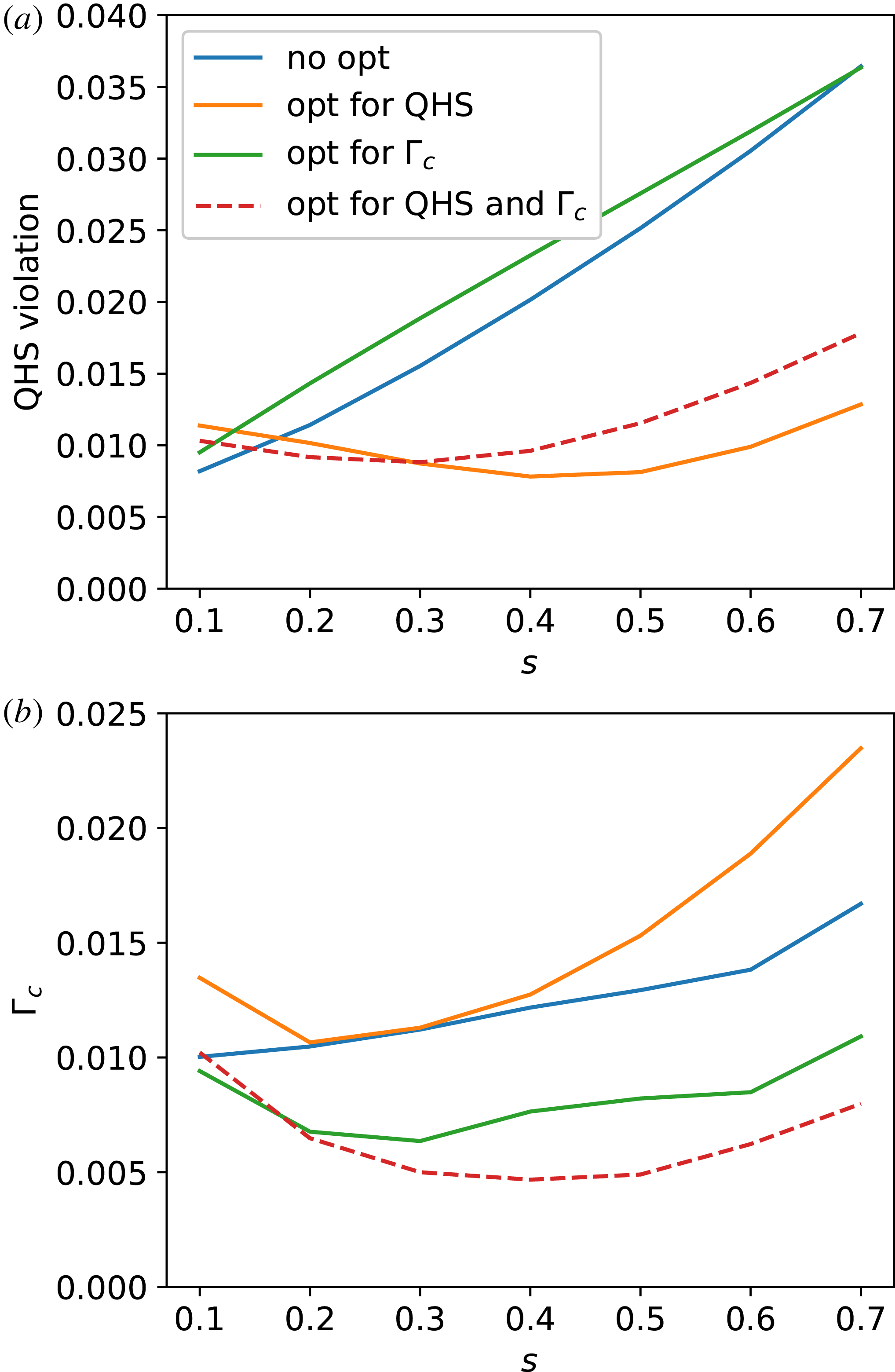
Figure 1(a) shows the values for the quasisymmetric metric computed for each of the four optimization cases and plotted as a function of
 $s$
. For these results and all similar plots, even though the values may have been optimized on only one surface (for QHS) or three surfaces (for
$s$
. For these results and all similar plots, even though the values may have been optimized on only one surface (for QHS) or three surfaces (for
 $\unicode[STIX]{x1D6E4}_{c}$
) we show the values of the metric at surfaces between
$\unicode[STIX]{x1D6E4}_{c}$
) we show the values of the metric at surfaces between
 $s=0.1$
and
$s=0.1$
and
 $s=0.7$
. The two optimizations that include quasisymmetry as a penalty, (orange and red) show lower values of quasisymmetry over the entirety of the minor radius, except possibly in the very core. Note the broad reduction despite that the optimization only targeted quasisymmetry at
$s=0.7$
. The two optimizations that include quasisymmetry as a penalty, (orange and red) show lower values of quasisymmetry over the entirety of the minor radius, except possibly in the very core. Note the broad reduction despite that the optimization only targeted quasisymmetry at
 $s=0.6$
. This behaviour is typical for optimization for quasisymmetry.
$s=0.6$
. This behaviour is typical for optimization for quasisymmetry.


Figure 1(b) shows a similar plot, but this time the
 $\unicode[STIX]{x1D6E4}_{c}$
metric is plotted as a function of
$\unicode[STIX]{x1D6E4}_{c}$
metric is plotted as a function of
 $s$
. Again the two cases that included the
$s$
. Again the two cases that included the
 $\unicode[STIX]{x1D6E4}_{c}$
metric in the optimization (green and red) show lower values of
$\unicode[STIX]{x1D6E4}_{c}$
metric in the optimization (green and red) show lower values of
 $\unicode[STIX]{x1D6E4}_{c}$
across most of the plasma. It appears from this result that the quasisymmetric metric and
$\unicode[STIX]{x1D6E4}_{c}$
across most of the plasma. It appears from this result that the quasisymmetric metric and
 $\unicode[STIX]{x1D6E4}_{c}$
can be optimized separately. Indeed, the following four configurations provide a good test case for comparing the behaviour of these two metrics on energetic particle confinement. The flux surfaces for the four configurations are shown in figure 2(a). The rotational transforms for the four configurations are shown in figure 2(b). The results show that even though the rotational transform was not explicitly targeted in the optimization, the configurations have rotational transforms between the low-order rational surfaces of
$\unicode[STIX]{x1D6E4}_{c}$
can be optimized separately. Indeed, the following four configurations provide a good test case for comparing the behaviour of these two metrics on energetic particle confinement. The flux surfaces for the four configurations are shown in figure 2(a). The rotational transforms for the four configurations are shown in figure 2(b). The results show that even though the rotational transform was not explicitly targeted in the optimization, the configurations have rotational transforms between the low-order rational surfaces of ![]() and
and ![]()

Figure 2. Flux surfaces are shown at toroidal cuts at
 $\unicode[STIX]{x1D719}=0$
,
$\unicode[STIX]{x1D719}=0$
,
 $\unicode[STIX]{x03C0}/8$
and
$\unicode[STIX]{x03C0}/8$
and
 $\unicode[STIX]{x03C0}/4$
(a). The magnetic axis is shown for the unoptimized case as a blue ‘
$\unicode[STIX]{x03C0}/4$
(a). The magnetic axis is shown for the unoptimized case as a blue ‘
 $+$
’. The colours in this plot use the same legend as in the bottom plot. Panel (b) shows the rotational transform as a function of normalized toroidal flux for four different optimization targets.
$+$
’. The colours in this plot use the same legend as in the bottom plot. Panel (b) shows the rotational transform as a function of normalized toroidal flux for four different optimization targets.
The evaluation for energetic particles is shown for particles beginning on the
 $s=0.1$
, 0.3 and 0.4 flux surfaces in figure 3. In the core, at
$s=0.1$
, 0.3 and 0.4 flux surfaces in figure 3. In the core, at
 $s=0.1$
(figure 3
a) corresponding to normalized minor radius,
$s=0.1$
(figure 3
a) corresponding to normalized minor radius,
 $r/a\sim 0.32$
, all configurations show losses below 4 % after 200 ms. The best performing case (red dashed) completely eliminates all alpha particle losses on this flux surface. For all configurations after about 10 ms the particle loss fraction is saturated.
$r/a\sim 0.32$
, all configurations show losses below 4 % after 200 ms. The best performing case (red dashed) completely eliminates all alpha particle losses on this flux surface. For all configurations after about 10 ms the particle loss fraction is saturated.

Figure 3. Alpha particle loss fractions for alpha particles born on the
 $s=0.1$
(a),
$s=0.1$
(a),
 $s=0.3$
(b) and
$s=0.3$
(b) and
 $s=0.4$
(c) surfaces as a function of time for four different optimization cases.
$s=0.4$
(c) surfaces as a function of time for four different optimization cases.
Further out, at
 $s=0.3$
(figure 3
b), corresponding to
$s=0.3$
(figure 3
b), corresponding to
 $r/a\sim 0.54$
, some differences can be seen between the four cases. The best performing case (red dashed) again shows low losses. No particles are lost before about 20 ms, and less than 1 % loss exists after 200 ms. The other configurations perform worse both with regard to prompt losses and after long time scales. All three other cases show approximately 7 % loss after 200 ms. Interestingly a clear difference appears in the time behaviour between the configuration optimized for
$r/a\sim 0.54$
, some differences can be seen between the four cases. The best performing case (red dashed) again shows low losses. No particles are lost before about 20 ms, and less than 1 % loss exists after 200 ms. The other configurations perform worse both with regard to prompt losses and after long time scales. All three other cases show approximately 7 % loss after 200 ms. Interestingly a clear difference appears in the time behaviour between the configuration optimized for
 $\unicode[STIX]{x1D6E4}_{c}$
(green) and the unoptimized case (blue) and the case optimized for quasisymmetry (orange). After 10 ms, the optimization for
$\unicode[STIX]{x1D6E4}_{c}$
(green) and the unoptimized case (blue) and the case optimized for quasisymmetry (orange). After 10 ms, the optimization for
 $\unicode[STIX]{x1D6E4}_{c}$
(green) performs significantly better than the other two, indicating an improvement in confining prompt losses of particles. However after 200 ms it performs slightly worse.
$\unicode[STIX]{x1D6E4}_{c}$
(green) performs significantly better than the other two, indicating an improvement in confining prompt losses of particles. However after 200 ms it performs slightly worse.
The trends continue further out at
 $s=0.4$
(figure 3
c), corresponding to
$s=0.4$
(figure 3
c), corresponding to
 $r/a\sim 0.63$
. At
$r/a\sim 0.63$
. At
 $s=0.4$
, the losses from the configuration with optimization for
$s=0.4$
, the losses from the configuration with optimization for
 $\unicode[STIX]{x1D6E4}_{c}$
and quasisymmetry is about 1 % after 10 ms and 3 % after 200 ms. Similar behaviour is seen with the case optimized for
$\unicode[STIX]{x1D6E4}_{c}$
and quasisymmetry is about 1 % after 10 ms and 3 % after 200 ms. Similar behaviour is seen with the case optimized for
 $\unicode[STIX]{x1D6E4}_{c}$
where it reduces prompt losses, but after 200 ms performs equivalently to the other two cases with approximately 8 % losses.
$\unicode[STIX]{x1D6E4}_{c}$
where it reduces prompt losses, but after 200 ms performs equivalently to the other two cases with approximately 8 % losses.
It is clear from these results that quasihelically symmetric configurations exist that have VMEC equilibria that eliminate all alpha particle losses within
 $s=0.1$
on an ARIES-CS scale device. The configuration was obtained with a basic set of optimization targets, using only the quasisymmetry metric and the
$s=0.1$
on an ARIES-CS scale device. The configuration was obtained with a basic set of optimization targets, using only the quasisymmetry metric and the
 $\unicode[STIX]{x1D6E4}_{c}$
metric.
$\unicode[STIX]{x1D6E4}_{c}$
metric.
We now turn towards some of the features of the optimized equilibria. One of the basic results is that improvements to energetic particle confinement are not correlated to improvements in neoclassical transport given by
 $\unicode[STIX]{x1D716}_{\text{eff}}$
. In figure 4 we show the computed values of
$\unicode[STIX]{x1D716}_{\text{eff}}$
. In figure 4 we show the computed values of
 $\unicode[STIX]{x1D716}_{\text{eff}}$
for the four optimization configurations, which demonstrates that the optimization which produced the best energetic particle confinement actually has the worst predicted neoclassical transport over the inner half of the plasma. It should be noted, that more accurate neoclassical calculations are available, such as with SFINCS (Landreman et al.
Reference Landreman, Smith, Mollén and Helander2014). These calculations have not been undertaken for these configurations. Rather the conclusion here is with regard to the limitation of
$\unicode[STIX]{x1D716}_{\text{eff}}$
for the four optimization configurations, which demonstrates that the optimization which produced the best energetic particle confinement actually has the worst predicted neoclassical transport over the inner half of the plasma. It should be noted, that more accurate neoclassical calculations are available, such as with SFINCS (Landreman et al.
Reference Landreman, Smith, Mollén and Helander2014). These calculations have not been undertaken for these configurations. Rather the conclusion here is with regard to the limitation of
 $\unicode[STIX]{x1D716}_{\text{eff}}$
as a useful metric for energetic particles.
$\unicode[STIX]{x1D716}_{\text{eff}}$
as a useful metric for energetic particles.

Figure 4. The
 $\unicode[STIX]{x1D716}_{\text{eff}}$
metric as a function of normalized toroidal flux for four different optimization targets.
$\unicode[STIX]{x1D716}_{\text{eff}}$
metric as a function of normalized toroidal flux for four different optimization targets.
It is also useful to look at the loss as a function of the value of field that the alpha particle will reflect at,
 $E/\unicode[STIX]{x1D707}$
, which is directly related to the particle’s pitch angle. The results for
$E/\unicode[STIX]{x1D707}$
, which is directly related to the particle’s pitch angle. The results for
 $s=0.3$
and
$s=0.3$
and
 $s=0.4$
are shown in figure 5. For both cases only trapped particles are lost, which is expected. Two more interesting features are apparent from the results presented here. The first is that for all configurations the losses are predominately from particles near the trapped–passing boundary. These losses are significantly reduced when
$s=0.4$
are shown in figure 5. For both cases only trapped particles are lost, which is expected. Two more interesting features are apparent from the results presented here. The first is that for all configurations the losses are predominately from particles near the trapped–passing boundary. These losses are significantly reduced when
 $\unicode[STIX]{x1D6E4}_{c}$
and quasisymmetry are both optimized for (red). However, in this best performing case there are some losses of deeply trapped particles at
$\unicode[STIX]{x1D6E4}_{c}$
and quasisymmetry are both optimized for (red). However, in this best performing case there are some losses of deeply trapped particles at
 $s=0.4$
. This may be expected due to the degradation of
$s=0.4$
. This may be expected due to the degradation of
 $\unicode[STIX]{x1D716}_{\text{eff}}$
in this case. In other words, the optimizer sacrificed some confinement of deeply trapped particles to improve confinement of energetic particles near the trapped–passing boundary. This is a good trade-off for particles born uniformly on flux surfaces, like alphas. Deeply trapped particles can only be born in areas of low magnetic field, while barely trapped particles can be born at all locations on the flux surface.
$\unicode[STIX]{x1D716}_{\text{eff}}$
in this case. In other words, the optimizer sacrificed some confinement of deeply trapped particles to improve confinement of energetic particles near the trapped–passing boundary. This is a good trade-off for particles born uniformly on flux surfaces, like alphas. Deeply trapped particles can only be born in areas of low magnetic field, while barely trapped particles can be born at all locations on the flux surface.

Figure 5. Loss counts as a function of reflecting field (
 $E/\unicode[STIX]{x1D707}$
) for alpha particles for four different optimizations. Values are calculated for particles launched at flux surfaces
$E/\unicode[STIX]{x1D707}$
) for alpha particles for four different optimizations. Values are calculated for particles launched at flux surfaces
 $s=0.3$
(a) and
$s=0.3$
(a) and
 $s=0.4$
(b). The black vertical dashed line in each plot represents the trapped–passing boundary.
$s=0.4$
(b). The black vertical dashed line in each plot represents the trapped–passing boundary.
Comparing this optimization attempt with previous attempts by Ku & Garabedian (Reference Ku and Garabedian2006) and Nemov et al. (Reference Nemov, Kasilov and Kernbichler2014) yield some insights. In this optimization, the original equilibrium is a scaled version of NCSX and suffered from energetic particle losses at all pitch values. A salient feature of the optimized equilibrium was the removal of magnetic wells at intermediate pitch values, thus producing a class of confined energetic particles. However, this process degraded quasisymmetry and introduced mirror modes, that is modes in the magnetic spectrum with poloidal number,
 $m=0$
and toroidal number
$m=0$
and toroidal number
 $n\neq 0$
. For the quasihelically symmetric configurations in this paper, there are very few losses at intermediate field values (see figure 5,
$n\neq 0$
. For the quasihelically symmetric configurations in this paper, there are very few losses at intermediate field values (see figure 5,
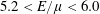 $5.2<E/\unicode[STIX]{x1D707}<6.0$
). Therefore, there are no improvements to be had by improving confinement in these regions of phase space since the particles are already well confined.
$5.2<E/\unicode[STIX]{x1D707}<6.0$
). Therefore, there are no improvements to be had by improving confinement in these regions of phase space since the particles are already well confined.
A different optimization by Nemov et al. (Reference Nemov, Kasilov and Kernbichler2014) attempted to remove losses due to coil-ripple effects. They showed that in HSX, the transition from an idealized quasisymmetric equilibrium to one produced from realistic coils significantly reduced energetic particle confinement. However, by doubling the number of coils from 48 to 96 using a simple interpolation scheme, the original good confinement was recovered. This occurred even though the new coils were not optimized and quasisymmetry was degraded in the 96 coil configuration.
4.1 Optimization at higher aspect ratios
The configurations presented above were all at aspect ratio 6.7. While larger than ARIES-CS, the aspect ratio is significantly smaller than that of the HELIAS reactor concept (Warmer et al.
Reference Warmer, Beidler, Dinklage and Wolf2016) which has aspect ratio 12.2 and plasma volume of
 ${\sim}1800~\text{m}^{3}$
.
${\sim}1800~\text{m}^{3}$
.
We attempted to optimize the equilibrium at higher aspect ratios, but keeping the plasma volume equivalent to the ARIES-CS value of
 $450~\text{m}^{3}$
. The methodology was to begin with an internal surface of an optimized case at aspect ratio 6.7 and then scale the boundary coefficients such that the volume was equivalent. The boundary surfaces for these equilibria are shown in figure 6 and the alpha particle losses are shown in figure 7 for
$450~\text{m}^{3}$
. The methodology was to begin with an internal surface of an optimized case at aspect ratio 6.7 and then scale the boundary coefficients such that the volume was equivalent. The boundary surfaces for these equilibria are shown in figure 6 and the alpha particle losses are shown in figure 7 for
 $0.1<s<0.5$
. Despite the decrease in minor radius, the higher aspect ratio configurations display better confinement. At low aspect ratios, it is more difficult to meet quasihelically symmetric targets.
$0.1<s<0.5$
. Despite the decrease in minor radius, the higher aspect ratio configurations display better confinement. At low aspect ratios, it is more difficult to meet quasihelically symmetric targets.

Figure 6. Boundary flux surfaces for the bean (
 $\unicode[STIX]{x1D719}=0$
) and triangle (
$\unicode[STIX]{x1D719}=0$
) and triangle (
 $\unicode[STIX]{x1D719}=\unicode[STIX]{x03C0}/4$
) surfaces for three optimized configurations with different aspect ratios.
$\unicode[STIX]{x1D719}=\unicode[STIX]{x03C0}/4$
) surfaces for three optimized configurations with different aspect ratios.

Figure 7. Alpha particle losses after 200 ms for three optimized configurations with different aspect ratios.
5 Conclusion
Results presented in this paper demonstrate that stellarator equilibria exist which have very low energetic particle losses within the half-radius with losses eliminated entirely within the
 $s=0.1$
surface. Therefore, in the core, stellarator equilibria can confine energetic particles equally well to idealized axisymmetric configurations, such as tokamaks without coil ripple. This potentially eliminates one of the major concerns with stellarator reactors, namely large wall loading from prompt losses of alpha particles.
$s=0.1$
surface. Therefore, in the core, stellarator equilibria can confine energetic particles equally well to idealized axisymmetric configurations, such as tokamaks without coil ripple. This potentially eliminates one of the major concerns with stellarator reactors, namely large wall loading from prompt losses of alpha particles.
These equilibria were created using an optimization recipe that sought to minimize non-symmetric components of the magnetic field spectrum and used the
 $\unicode[STIX]{x1D6E4}_{c}$
metric proposed by Nemov to minimize collisionless energetic particle losses. The results showed that optimization with both the
$\unicode[STIX]{x1D6E4}_{c}$
metric proposed by Nemov to minimize collisionless energetic particle losses. The results showed that optimization with both the
 $\unicode[STIX]{x1D6E4}_{c}$
metric and quasihelical symmetry produced configurations with very low energetic particle losses, including the elimination of all losses within approximately the mid-radius. However, the best performing case loses some deeply trapped particles at the
$\unicode[STIX]{x1D6E4}_{c}$
metric and quasihelical symmetry produced configurations with very low energetic particle losses, including the elimination of all losses within approximately the mid-radius. However, the best performing case loses some deeply trapped particles at the
 $s=0.4$
surface, where other configurations do not.
$s=0.4$
surface, where other configurations do not.
The results suggest that it is possible to achieve good energetic particle confinement despite an increase in the neoclassical metric,
 $\unicode[STIX]{x1D716}_{\text{eff}}$
by about a factor of 2 in the core. While
$\unicode[STIX]{x1D716}_{\text{eff}}$
by about a factor of 2 in the core. While
 $\unicode[STIX]{x1D716}_{\text{eff}}$
tends to focus on confining deeply trapped particles, energetic particles are often lost near the trapped–passing boundary. Indeed, it is possible to degrade neoclassical transport, as given by
$\unicode[STIX]{x1D716}_{\text{eff}}$
tends to focus on confining deeply trapped particles, energetic particles are often lost near the trapped–passing boundary. Indeed, it is possible to degrade neoclassical transport, as given by
 $\unicode[STIX]{x1D716}_{\text{eff}}$
, significantly, yet the overall energetic particle losses can be improved because of large reduction of losses near the trapped–passing boundary. This optimization can be contrasted with previous results from Ku & Garabedian (Reference Ku and Garabedian2006) and Nemov et al. (Reference Nemov, Kasilov and Kernbichler2014) who showed that it is possible to have improved energetic particle confinement despite reduced quasisymmetry. In Ku et al. this was accomplished by introducing
$\unicode[STIX]{x1D716}_{\text{eff}}$
, significantly, yet the overall energetic particle losses can be improved because of large reduction of losses near the trapped–passing boundary. This optimization can be contrasted with previous results from Ku & Garabedian (Reference Ku and Garabedian2006) and Nemov et al. (Reference Nemov, Kasilov and Kernbichler2014) who showed that it is possible to have improved energetic particle confinement despite reduced quasisymmetry. In Ku et al. this was accomplished by introducing
 $m=0$
,
$m=0$
,
 $n=3$
and
$n=3$
and
 $m=1$
,
$m=1$
,
 $n=3$
modes in order to improve energetic particle confinement. In Nemov et al. it was accomplished by increasing the number of modular coils to reduce the coil-ripple term.
$n=3$
modes in order to improve energetic particle confinement. In Nemov et al. it was accomplished by increasing the number of modular coils to reduce the coil-ripple term.
This paper represents new progress on energetic particle confinement optimization in stellarators. Stellarator equilibrium optimization always requires trade-offs between different desired properties. A more comprehensive analysis is needed to determine the compatibility of good energetic ion physics with other confinement properties. It may be true that other desirable properties conflict with good energetic particle confinement. A full analysis is necessary.
The calculations were performed using collisionless drift orbits which represent optimistic estimates of particle losses. More realistic simulations would include both the slowing down of the alpha particles and pitch angle scattering. Collisional calculations require knowledge of the plasma temperature and density as a function of flux surface and will be a subject of future work.
Additionally, the effect of energetic particle modes, such as those in the Alfvén eigenmode family were not considered here. Investigating alpha particle instabilities will be important for reactors. For an overview of current research on energetic particle modes in stellarators, and the possibility of achieving reduced mode drive due to operation at higher density, see § 2.5 of Gates et al. (Reference Gates, Anderson, Anderson, Zarnstorff, Spong, Weitzner, Neilson, Ruzic, Andruczyk and Harris2018).
Also, all the quasihelically symmetric equilibria presented were vacuum magnetic configurations. A requirement for quasisymmetric equilibria is that good confinement is needed from the starting vacuum configuration up to the full performance with both finite
 $\unicode[STIX]{x1D6FD}$
effects and bootstrap currents. Producing such equilibria was not attempted here.
$\unicode[STIX]{x1D6FD}$
effects and bootstrap currents. Producing such equilibria was not attempted here.
So far, all the results presented are for idealized configurations that do not include the effects of magnetic field coils. Just as in tokamaks, coils produce additional ripple-trapped particles and constitute an additional loss mechanism. The coil-ripple effect is important, but was beyond the scope of this paper. Nevertheless, we describe here two possible methods of addressing the coil-ripple effects.
One of the more difficult aspects of stellarator coil design is maximizing the coil–plasma distance. In a reactor, the minimum size of the device will most likely be set by the neutronics blanket that must be between the vacuum and the plasma. A key parameter is the minimal coil–plasma separation distance, and this is a target to maximize (El-Guebaly et al. Reference El-Guebaly, Raffray, Malang, Lyon and Ku2005). It is possible to identify regions where coil position is most sensitive (Landreman & Paul Reference Landreman and Paul2018; Paul et al. Reference Paul, Landreman, Bader and Dorland2018), and it may be possible to target equilibria to relax specific regions such as those with strong concavities (see § 7 of Paul et al. Reference Paul, Landreman, Bader and Dorland2018). Furthermore, in regions where the coil’s position is less sensitive, such as the low-field side on the outside of the device, it is possible to move coils further away. This should lower the coil ripple in these regions and the expectation is that it should lower alpha particle losses from ripple-trapped particles.
A second approach is to use ferritic inserts for stellarators similar to the use in tokamaks (Shinohara et al. Reference Shinohara, Tani, Oikawa, Putvinski, Schaffer and Loarte2012). Ferritic inserts have so far not been designed for stellarators, and it is an open area of research. This could be a promising approach to reduce coil-ripple losses.
Acknowledgements
The work for this paper was supported by DE-FG02-93ER54222, DE-FG02-99ER54546 and UW 2020 135AAD3116.