


1 Introduction
One of the critical areas of research supporting the successful operation of ITER and other large-current tokamaks is the development of techniques to mitigate the high thermal and magnetic energies released in plasma-terminating disruptions (Boozer Reference Boozer2015). The heat loads resulting from the sudden loss of thermal energy – the thermal quench (TQ) – and the electromechanical stresses induced by the subsequent loss of the plasma current – the current quench (CQ) – might cause severe damage to plasma-facing components (Lehnen et al. Reference Lehnen, Aleynikova, Aleynikov, Campbell, Drewelow, Eidietis, Gasparyan, Granetz, Gribov and Hartmann2015).
Massive material injection (MMI) has been considered as a possible method to safely terminate the discharge and avoid disruption-related damage (Hollmann et al. Reference Hollmann, Aleynikov, Fülöp, Humphreys, Izzo, Lehnen, Lukash, Papp, Pautasso and Saint-Laurent2015). When injected into a disrupting plasma, impurity atoms radiate energy away from the plasma isotropically, thereby reducing localized heat loads. The choice of the impurity, quantity and injection scheme provides means to control the CQ duration to a certain extent. This is important since the CQ duration determines the magnitude of the induced eddy currents in the wall, and thus the related mechanical forces, together with the toroidal electric field responsible for the generation of runaway electrons (REs).
During the CQ phase of disruptions in reactor-scale devices, such as ITER, large RE currents are expected to form (Boozer Reference Boozer2015; Breizman et al. Reference Breizman, Aleynikov, Hollmann and Lehnen2019). These energetic electrons are of particular concern, as they may give rise to localized power deposition and cause melting of plasma-facing components. ITER will have approximately an order of magnitude higher plasma current compared to current devices, which makes a substantial difference in the potential e-folds of the seed current (Rosenbluth & Putvinski Reference Rosenbluth and Putvinski1997). As MMI has a major impact on the runaway dynamics, it is also being considered as a runaway mitigation method. However, no clear strategy regarding runaway mitigation with MMI has emerged yet.
Recent results of Hesslow et al. (Reference Hesslow, Embréus, Vallhagen and Fülöp2019a) indicate a substantial increase in the avalanche multiplication gain in the presence of MMI of heavy impurities compared to previous estimates. The reason is that in the presence of partially ionized impurities, the increased number of target electrons available for the avalanche multiplication of runaways is only partially compensated by the increased friction force.
In this paper, we address the runaway current formation in connection with material injection in ITER disruption scenarios. The simulations are performed with a one-dimensional runaway fluid code, based on the go framework, described in § 2. go has been used in the past for evaluating material injection scenarios (Gál et al. Reference Gál, Fehér, Smith, Fülöp and Helander2008; Fehér et al. Reference Fehér, Smith, Fülöp and Gál2011), and for interpretative modelling of experiments (Papp et al. Reference Papp, Fülöp, Fehér, de Vries, Riccardo, Reux, Lehnen, Kiptily, Plyusnin and Alper2013). The version used in this paper includes Dreicer, tritium decay and Compton contributions to the runaway seed formation, and avalanche generation. A careful modelling of the effect of partially ionized atoms is particularly important as we consider heavy noble gas impurities. Thus, we use the avalanche growth rate derived by Hesslow et al. (Reference Hesslow, Embréus, Vallhagen and Fülöp2019a), which has been carefully benchmarked to kinetic simulations. In § 3, we present simulations in ITER scenarios, with neon and argon impurity injections, as well as mixed impurity–deuterium injections.
The model used here contains self-consistent calculations of the temperature and electric field evolution during the CQ, including the main runaway generation mechanisms except hot-tail generation. The omission of part of the hot-tail source is motivated with radial losses due to the breakup of magnetic surfaces that accompanies the TQ. Indeed, recent work based on fluid-kinetic simulations shows that taking into account all the hot-tail electrons overestimates the final runaway current by a factor of approximately four in ASDEX Upgrade (Hoppe et al. Reference Hoppe, Hesslow, Embreus, Unnerfelt, Papp, Pusztai, Fülöp, Lexell, Lunt and Macusova2020). Even if it is difficult to know how large a part of the hot-tail runaways become deconfined in an ITER TQ, it is reasonable to assume that some of the hot-tail seed survives. Indeed, deeply trapped electrons do not get lost even when the magnetic surfaces break up, and can be scattered into the passing region and run away after the magnetic surfaces have re-formed. Therefore, the model presented here is likely to underestimate the runaway seed.
Even in the absence of the hot-tail seed, our results indicate that if losses due to magnetic perturbations do not occur during a large fraction of the CQ, impurity injection leads to high runaway currents in the deuterium–tritium (DT) phase of ITER operation, even if it is combined with deuterium injection. The reason is that the cooling associated with a large amount of injected material results in low temperatures leading to recombination and corresponding high value of the total-to-free electron density ratio, which in turn enhances the avalanche growth rate. A consequence of these results is that successful runaway mitigation during the non-nuclear phase of ITER operation may not provide a sufficient validation of the ITER disruption mitigation strategy, since the presence of radioactive sources of superthermal electrons during the DT phase changes the dynamics.
2 Current dynamics and temperature evolution during material injection
In a cooling plasma, the conductivity drops and an electric field is induced to maintain the plasma current. The evolution of the parallel electric field  $E_\|$ is modelled by the flux-surface averaged induction equation (Fülöp et al. Reference Fülöp, Helander, Vallhagen, Embreus, Hesslow, Svensson, Creely, Howard and Rodriguez-Fernandez2020)
 \begin{equation} \frac{1+\kappa^{-2}}{2}\frac{1}{r}\frac{\partial }{\partial r} r\frac{\partial E_\|}{\partial r}=\mu_0 \frac{\partial j_\parallel}{\partial t},\end{equation}
where  $\kappa$ is the elongation (assumed to be constant here) and $j_\parallel =\sigma _\textrm {Sp} E_\|+j_\textrm {RE}\approx \sigma _\textrm {Sp} E_\|+ecn_\textrm {RE}$ is the sum of Ohmic and runaway current densities, with $n_\textrm {RE}$ being the number density, $j_\textrm {RE}$ the current density of runaways and $\sigma _\textrm {Sp}$ the Spitzer conductivity. Furthermore, $r$ denotes the minor radius at the mid-plane, while $\mu _0$, $e$ and $c$ denote the magnetic permeability, the elementary charge and the speed of light, respectively. The boundary conditions for (2.1) are $\partial E_\parallel /\partial r|_{r=0}=0$, while at $r=a$, where $a=2\ \textrm {m}$ is the mid-plane minor radius of the plasma, $E_\parallel$ is determined by a perfectly conducting wall at $r=b=2.15\ \textrm {m}$. Matching the solution for $r < a$ to the vacuum solution for $a < r < b$ gives $E_\parallel (a)=a\ln {(a/b)}\partial E_\parallel /\partial r|_{r=a}$. Note that $j_\|$ and $E_\|$ represent flux-surface averaged values. Toroidicity effects are neglected here.
When the electric field is larger than a critical field, runaways are produced by velocity space diffusion into the runaway region due to small-angle collisions (Dreicer generation), and, in DT operation, by tritium decay and Compton scattering of  $\gamma$ photons originating from the activated wall. In addition, existing runaways can create new ones through close collisions with lower-energy electrons (Rosenbluth & Putvinski Reference Rosenbluth and Putvinski1997). The resulting exponential growth in the number of REs – the avalanche – can be substantially increased in disruptions mitigated by MMI, according to recent estimates by Hesslow et al. (Reference Hesslow, Embréus, Vallhagen and Fülöp2019a).
2.1 Runaway generation rates
To compute the Dreicer runaway generation rate for given plasma conditions, we use a neural networkFootnote 1 (Hesslow et al. Reference Hesslow, Unnerfelt, Vallhagen, Embreus, Hoppe, Papp and Fülöp2019b) trained on a large number of kinetic simulations by the code kinetic equation solver (Landreman, Stahl & Fülöp Reference Landreman, Stahl and Fülöp2014), which accounts for the effect of partially ionized atoms as described by Hesslow et al. (Reference Hesslow, Embréus, Hoppe, DuBois, Papp, Rahm and Fülöp2018a). In ITER-like disruptions we find, however, that Dreicer generation is always negligible compared to the other reactor-relevant seed generation mechanisms, hot-tail generation, tritium decay and Compton scattering, but for completeness it is included in the simulations.
The runaway seed produced by tritium decay is modelled as (Martín-Solís, Loarte & Lehnen Reference Martín-Solís, Loarte and Lehnen2017; Fülöp et al. Reference Fülöp, Helander, Vallhagen, Embreus, Hesslow, Svensson, Creely, Howard and Rodriguez-Fernandez2020)
 \begin{equation} \left(\frac{\partial n_\textrm{RE}}{\partial t}\right)^\textrm{tritium}=\ln{(2)}\frac{n_\textrm{T}}{\tau_\textrm{T}}f(W_\textrm{crit}),\end{equation}
where  $n_\textrm {T}$ is the tritium density, $\tau _\textrm {T}\approx 4500$ days is the half-life of tritium and $f(W_\textrm {crit})\approx 1-(35/8)w^{3/2}+(21/4)w^{5/2}-(15/8)w^{7/2}$ is the fraction of the electrons created by tritium decay above the critical runaway energy $W_\textrm {crit}$, with $w=W_\textrm {crit}/Q$ and $Q=18.6\ \textrm {keV}$. The critical runaway energy $W_\textrm {crit}$ is given by $W_\textrm {crit}=m_\textrm {e} c^2(\sqrt {p_\star ^2+1}-1)$, in terms of
 \begin{equation} p_\star = \sqrt[4]{\bar{\nu}_{s}(p_\star) \bar{\nu}_\textrm{D}(p_\star)}/\sqrt{E_\parallel/E_{c} },\end{equation}
the critical momentum for runaway acceleration, where the runaway probability makes a rapid transition between values of essentially  $0$ and $1$, as shown in appendix A. We normalize momenta to $m_\textrm {e} c$, and we have introduced the critical electric field $E_\textrm {c}=n_\textrm {e} e^3 \ln \varLambda_c /(4 {\rm \pi}\epsilon _0^2 m_\textrm {e} c^2)$, where $n_\textrm {e}$ is the free electron density, $\ln \varLambda _{c} \approx 14.6+0.5 \ln (T_\textrm {eV}/n_\textrm {e20})$ is the relativistic Coulomb logarithm, $T_\textrm {eV}$ is the electron temperature in electronvolts and $n_\textrm {e20}$ is the density of the background electrons in units of $10^{20}\ \textrm {m}^{-3}$, $\epsilon _0$ is the vacuum permittivity and $m_\textrm {e}$ is the electron mass.
Here, the normalized slowing-down and deflection frequencies,  $\bar {\nu }_{s}$ and $\bar {\nu }_\textrm {D}$, are defined in terms of the full ones ( $\nu _\textrm {s}$ and $\nu _\textrm {D}$) through (5) and (9) of (Hesslow et al. Reference Hesslow, Embréus, Wilkie, Papp and Fülöp2018b):
 \begin{equation} \nu_\textrm{s} = \frac{eE_\textrm{c}}{m_\textrm{e} c}\frac{\gamma^2}{p^3}\bar\nu_\textrm{s}, \quad \nu_\textrm{D} =\frac{eE_\textrm{c}}{m_\textrm{e} c}\frac{\gamma }{p^3}\bar\nu_\textrm{D}. \end{equation}
In the case of a fully ionized plasma and with a constant Coulomb logarithm,  $\bar \nu _\textrm {s} = 1$ and $\bar \nu _\textrm {D} = 1+Z_\textrm {eff}$.
Runaways can also be created via Compton scattering of electrons to the runaway region in momentum space. These events are caused by  $\gamma$ photons emitted from the plasma-facing components that are activated by the neutrons produced in the DT fusion reactions. Using radiation transport calculations performed at several poloidal locations in ITER, Martín-Solís et al. (Reference Martín-Solís, Loarte and Lehnen2017) estimated the gamma flux energy spectrum to be $\varGamma _\gamma (E_\gamma ) =\varGamma _{\gamma 0} \exp {(-\exp {(z)}-z+1)}$, with $z=[\ln {(E_\gamma [\textrm {MeV}])}+1.2]/0.8$ and $\varGamma _{\gamma 0}=4.44\times 10^{17}\ \textrm {m}^{-2}\,\textrm {s}^{-1}\,\textrm {MeV}^{-1}$, giving a total flux of $10^{18}\ \textrm {m}^{-2}\,\textrm {s}^{-1}$, when integrated over energy. Using the expression for the total Compton cross-section (Martín-Solís et al. Reference Martín-Solís, Loarte and Lehnen2017)
 \begin{align} \sigma(E_\gamma)&= \frac{3 \sigma_\textrm{T}}{8}\left\{ \frac{x^2-2x-2}{x^3}\ln{\frac{1+2x}{1+x(1-\cos{\theta_\textrm{c}})}}\right.\nonumber\\ &\quad \left.+ \frac{1}{2x}\left[\frac{1}{\left[1+x(1-\cos{\theta_\textrm{c}})\right]^2}-\frac{1}{(1+2x)^2}\right]\right.\nonumber\\ &\quad \left.-\frac{1}{x^3}\left[1-x-\frac{1+2x}{1+x(1-\cos{\theta_\textrm{c}})}-x \cos{\theta_\textrm{c}}\right]\right\}, \end{align}
with
 \begin{equation} \cos{\theta_\textrm{c}}=1-\frac{m_\textrm{e} c^2}{E_\gamma} \frac{W_\textrm{crit}/E_\gamma}{1-(W_\textrm{crit}/E_\gamma)}, \end{equation}
the Thomson scattering cross-section  $\sigma _\textrm {T}=8{\rm \pi} /3[e^2/(4{\rm \pi} \epsilon _0m_\textrm {e} c^2)]^2$ and $x=E_\gamma /(m_\textrm {e} c^2)$, the runaway generation rate can be evaluated as
 \begin{equation} \left(\frac{\partial n_\textrm{RE}}{\partial t}\right)^\gamma =n_\textrm{e} \int\varGamma_\gamma (E_\gamma)\sigma (E_\gamma)\, \textrm{d} E_\gamma. \end{equation}
Note that the Compton seed depends on the final configuration of the first wall and blanket, as well as the time elapsed after the DT reactions cease; therefore the numbers used here are only estimates.
Close collisions between existing runaways and thermal electrons generate new runaways, leading to an exponential growth of the runaway density, from a usually tiny seed population. In partially ionized plasmas, the growth rate for this avalanche process is influenced by the extent to which fast electrons can penetrate the bound electron cloud around the impurity ion, i.e. the effect of partial screening. Taking into account these effects, the growth rate is given by (Hesslow et al. Reference Hesslow, Embréus, Vallhagen and Fülöp2019a)
 \begin{equation} \left(\frac{\partial n_\textrm{RE}}{\partial t}\right)_\textrm{aval}^\textrm{screened} = \frac{en_\textrm{RE}}{m_{e} c \ln\varLambda_{c}} \frac{n_{e}^\textrm{tot}}{n_{e}} \frac{E_\parallel-{E_{c}^\textrm{eff}}}{\sqrt{4+ \bar{\nu}_{s}(p_\star) \bar{\nu}_\textrm{D}(p_\star) }},\end{equation}
where  $n_{e}$ and $n_{e}^\textrm {tot}$ are the free and the total (free+bound) electron densities, respectively (Hesslow et al. Reference Hesslow, Embréus, Hoppe, DuBois, Papp, Rahm and Fülöp2018a). The expression for $ ({E_{c}^\textrm {eff}})$ was derived in Hesslow et al. (Reference Hesslow, Embréus, Wilkie, Papp and Fülöp2018b)Footnote 2. To obtain a well-behaved formula also for $E_\parallel < {E_{c}^\textrm {eff}}$, which we use to approximately describe the runaway decay at near-critical electric fields (neglecting losses due to magnetic perturbations), we replace $p_\star (E_\parallel )$ by $p_\star ({E_{c}^\textrm {eff}})$ for $E_\parallel <{E_{c}^\textrm {eff}}$.
In the completely screened limit, when the electron only interacts with the net charge of the ion, the avalanche growth rate reduces to (Rosenbluth & Putvinski Reference Rosenbluth and Putvinski1997)
 \begin{equation} \left(\frac{\partial n_\textrm{RE}}{\partial t}\right)_\textrm{aval}^\textrm{RP}= \frac{e n_\textrm{RE}}{m_\textrm{e} c \ln\varLambda_{c}} \frac{E_\parallel-E_{c}}{\sqrt{5+Z_\textrm{eff}}}.\end{equation}
 The Dreicer and the avalanche runaway generation processes can be reduced by finite aspect ratio effects. However, recent results of McDevitt & Tang (Reference McDevitt and Tang2019) indicate that at high densities and electric fields this reduction is negligible due to the high collisionality of electrons at momentum  $p_\star$. In such circumstances, the bounce-averaged approach for collisionless electrons, previously employed to take into account the effect of toroidicity, is not valid, and the runaway generation is approximately local. As we consider cases with MMI, leading to high densities, in this paper the commonly used neoclassical factor that would multiply the avalanche growth rate ( $\varphi _\epsilon =(1+1.46\epsilon ^{1/2}+1.72 \epsilon )^{-1/2}$, with $\epsilon$ the inverse aspect ratio) will be omitted.
Hot-tail generation occurs in the case of sudden cooling, when the collision frequency is lower than the cooling rate, and fast electrons do not have time to thermalize. Hot-tail generation is predicted to be the dominant primary generation when the TQ duration is shorter than the collision time at the runaway threshold velocity (Helander et al. Reference Helander, Smith, Fülöp and Eriksson2004), which is likely to be the case in ITER (Smith et al. Reference Smith, Helander, Eriksson and Fülöp2005). However, hot-tail runaways are produced in the early phase of the TQ when the level of magnetic fluctuations is high, and their losses due to radial transport are likely to be significant. Lacking reliable models for self-consistently treating the hot-tail generation and the losses due to magnetic fluctuations during the TQ, both of these processes will be ignored in this paper. The implications of a remnant hot-tail seed will be discussed in § 4.
2.2 Temperature evolution
The major causes of energy loss during disruption are radial transport due to magnetic fluctuations, induced by magnetohydrodynamic (MHD) instabilities, and line radiation due to impurity influx. The MHD-induced energy loss is likely to dominate in the initial part of the TQ until the temperature has dropped to  $\sim$100 eV, due to its strong temperature scaling ${\sim }T^{5/2}$ (Ward & Wesson Reference Ward and Wesson1992). For simplicity, this part of the temperature drop is modelled by an exponential decay according to
 \begin{equation} T(r,t)=T_\textrm{f}(r)+[T_0(r)-T_\textrm{f}(r)]\, \textrm{e}^{-t/t_0}, \end{equation}
where the temperature decays from the initial  $T_0(r)$ towards the final $T_\textrm {f}(r)$ temperature profile with a characteristic time constant $t_0$. This temperature evolution is employed until the central temperature drops to $\sim$100 eV. After this, the MHD-induced losses are assumed to be negligible, and the temperature evolution is determined by the energy balance equation
 \begin{align} \frac{3}{2}\frac{\partial (n T)}{\partial t}=\frac{1+\kappa^{-2}}{2}\frac{3 n}{2 r}\frac{\partial }{\partial r}\left(\chi r \frac{\partial T}{\partial r}\right)+\sigma(T, Z_\textrm{eff}) E^2-\sum_{i,k}n_\textrm{e}n_{k}^iL_{k}^i(T,n_\textrm{e})-P_\textrm{Br}-P_\textrm{ion}, \end{align}
where  $n$ is the total density of all species (electrons and ions), $n^k_{i}$ is the density of the $i$th charge state ( $i=0, 1,\ldots , Z-1$) of the ion species $k$ (e.g. deuterium, neon), $P_\textrm {Br}[\textrm {W\,m}^{-3}]= 1.69\times 10^{-38} (n_\textrm {e}[\textrm {m}^{-3}])^2 \sqrt {T[\textrm {eV}]} Z_\textrm {eff}$ is the Bremsstrahlung radiation loss and $P_\textrm {ion}=\sum _{i,k} E_k^i I_k^i n_k^i n_\textrm {e}$ is the ionization energy loss. Here, $I_k^{i}$ denotes the electron impact ionization rate and $R_k^i$ the radiative recombination rate for the $i$th charge state of species $k$, respectively, and $E_k^i$ denotes the corresponding ionization energy. The ionization and recombination rates, as well as the line radiation rates $L_k^{i}(n_\textrm {e},T)$, are extracted from the Atomic Data and Analysis Structure (ADAS) databaseFootnote 3 . The heat diffusion term in the equation is included for completeness, but its effect is negligible in all the considered cases. In the simulations we use the constant heat diffusion coefficient $\chi =1\ \textrm {m}^2\,\textrm {s}^{-1}$, but values in the range $0.1$– $100\ \textrm {m}^2\,\textrm {s}^{-1}$ give similar final runaway currents.
We calculate the density of each charge state for every ion species from the time-dependent rate equations
 \begin{equation} \frac{\textrm{d} n_{k}^i}{\textrm{d} t}= n_\textrm{e} [I_k^{i-1} n_{k}^{i-1} - (I_k^i+ R_k^i) n_{k}^{i} + R_k^{i+1} n_{k}^{i+1}].\end{equation}
To allow for comparison to previous work by Martín-Solís et al. (Reference Martín-Solís, Loarte and Lehnen2017), we will also show results using a temperature evolution assuming equilibrium between Ohmic heating and line radiation losses, so that the temperature profile satisfies
 \begin{equation} E^2\sigma[T,Z_\textrm{eff}(T)]=\sum_i n_\textrm{e}(T)n^i_k L^i_k [T,n_\textrm{e}(T)]. \end{equation}
Equation (2.13) is solved numerically using  $T=5$ eV as initial temperature. In this case, the densities of the various ionization states, and the corresponding electron density, are calculated assuming an equilibrium between ionization and recombination; that is, $n^{i}_k$ are computed from
 \begin{equation} \left. \begin{array}{c@{}} R^{i+1}_k n^{i+1}_k-I^i_k n^i_k=0, \quad i=0,1,\ldots,Z-1,\\ \displaystyle \sum_i n^{i}_k=n^\textrm{tot}_k, \quad i=0,1,\ldots Z, \end{array} \right\}\end{equation}
where  $n^\textrm {tot}_k$ is the total density of species $k$.
$k$.
3 Effect of massive material injection
In the following we present simulations of an ITER-like CQ with material injection. For the scenario we consider, the initial plasma current is  $I_\textrm {p}(t=0)=15\ \textrm {MA}$, and the major and minor radii are $R=6\ \textrm {m}$ and $a=2\ \textrm {m}$, respectively. The pre-disruption density profile is assumed to be flat with a value of $n_\textrm {e}(t=0)=10^{20}\ \textrm {m}^{-3}$. The initial temperature profile is given by $T(t=0,r) = 20 [1-(r/a)^2] \ \textrm {keV}$. The initial current density profile is assumed to be $j_\|(t=0,r)=j_{0} [1-(r/a)^{0.41}]$, with the normalization parameter $j_{0}$ chosen to give a total plasma current of $15\ \textrm {MA}$ (for a non-elongated plasma, $\kappa =1$, it is $j_{0}=1.69 \ \textrm {MA}\,\textrm {m}^{-2}$). The current density profile $j_\|(t=0,r)$ corresponds to an internal inductance of $l_{i}=0.7$. This set of initial plasma parameters is similar to that used by Martín-Solís et al. (Reference Martín-Solís, Loarte and Lehnen2017).
We solve the induction equation, (2.1), with the runaway generation rate given by the sum of the primary (Dreicer+tritium decay+Compton) and avalanche growth rates, for different amounts of impurity and deuterium. We find that the tritium or Compton seed dominates over Dreicer in all the considered cases.
The seed from tritium decay decreases with increasing impurity content. This is partly due to the shorter CQ times associated with higher impurity content, leaving the seed less time to be generated, and partly because the critical energy,  $W_\textrm {crit}$, increases with increasing impurity content, so that a smaller fraction of the tritium spectrum falls within the runaway region.
On the other hand, the Compton seed increases with increasing impurity content, due to the increasing number of available target electrons for Compton scattering. The energy of the  $\gamma$ photons is much larger than the ionization potential for all species present in the plasma, hence both bound and free electrons can become runaways due to Compton scattering. Furthermore, the energy of the $\gamma$ photons is much larger than the critical runaway energy, so an increase in the critical runaway energy only has a marginal effect on the runaway generation due to Compton scattering by preventing electrons scattered at large angles from becoming runaways.
As a result, a seed current of the order of a few amperes is obtained almost independently of the injected amount of noble gas and/or deuterium. As we will see, even if the seed current is very small, it results in a large final runaway current, due to the substantial avalanche effect.
We assume the injected material to be uniformly distributed at the beginning of the simulation. For the initial part of the TQ, we use an exponentially decaying temperature evolution according to (2.10) with  $t_0=1$ ms and $T_\textrm {f}(r)=50\,{\rm eV}$ (flat profile), until $t=6$ ms, when the central temperature has dropped to $\approx 100 \ \textrm {eV}$. This represents the initial phase of the disruption when the MHD-induced energy loss dominates. Below $100 \ \textrm {eV}$ the temperature is determined by the energy balance equation (2.11). The density of the charge states for every ion species is calculated from the time-dependent rate equations (2.12) during the whole simulation, both in the initial exponential decay phase and when the energy balance equation is employed. The main reason for using the exponentially decaying temperature in the initial phase is to determine the initial charge states of the impurities when the temperature reaches $100 \ \textrm {eV}$, and the energy balance equation is invoked. We have confirmed that the results are insensitive to the value of the decay time and the value of the heat diffusion coefficient $\chi$.
3.1 Pure neon injection
To illustrate the effect of impurity injection, we start by simulating the runaway dynamics for pure noble gas injections. Figure 1(a) shows the runaway current as a function of injected neon and argon density (normalized to the initial deuterium density,  $10^{20}\ \textrm {m}^{-3}$), using two models for avalanche generation: with partial screening effects, as given in (2.8), and with complete screening (2.9), respectively. The effect of screening is substantial. It increases the final runaway current from about $2$–
$2$– $3\ \textrm {MA}$ without screening to $6$–
$6$– $7\ \textrm {MA}$ with screening, for both neon and argon injections. Including partial screening, i.e. using (2.8), the avalanche growth rate increases with density for neon injection, while in the completely screened case, i.e. using (2.9), it is slightly decreasing. Including the effect of the elongation reduces the final runaway current at higher injected neon densities, but only marginally.

Figure 1. (a) Maximum runaway current as a function of injected noble gas density. Solid: neon with partial screening (i.e. avalanche calculated with (2.8)); dash-dotted: neon complete screening (‘CS’, i.e. using (2.9)); dotted: argon with partial screening; long dashed: argon complete screening; dashed: neon with partial screening at  $\kappa =1.6$. Panels (b–d) correspond to $10^{20}\ \textrm {m}^{-3}$ neon injection, with partial screening effects included and $\kappa =1$. (b) Temporal evolution of plasma current (solid), and breakdown into Ohmic (dash-dotted) and runaway (dashed) contributions. (c) Snapshots from the time evolution of the temperature. (d) Initial current profile (solid) and runaway current profile at the end of the Ohmic CQ (dashed).
Figure1(b–d) shows details of the current and temperature evolution during the CQ for a representative case with  $n_\textrm {Ne}=10^{20}$ m $^{-3}$. The temperature stabilizes at a few eV at the centre with a rather flat radial profile, resulting in a CQ time scale of the order of a few tens of milliseconds. The CQ is completed at $\sim$20 ms (14 ms after the TQ) and results in the formation of a runaway beam with a current of 6.7 MA. At this time the radial profile of the runaway beam is slightly more peaked around the magnetic axis compared to the initial current profile. The dissipation rate (after 20 ms) is very slow for this relatively modest injected impurity density.
3.2 Mixed deuterium and neon injection
We now turn to simulating the effect of injections of mixtures of noble gas and deuterium using the same approach as in the previous section. Runaway currents right before the dissipation phase (i.e. when  $I_\textrm {RE}$ assumes its maximum) are shown in figure 2, for different amounts of injected noble gas and deuterium. Below the green solid line the injected gas mixture is insufficient to induce a complete radiative collapse, which we characterize by requiring that the CQ time, defined as $t_\textrm {CQ}=[t(I_\textrm {Ohm}=0.2I_\textrm {p}^{(t=0)})-t(I_\textrm {Ohm}=0.8I_\textrm {p}^{(t=0)} )]/0.6$, is longer than $150\ \textrm {ms}$. For these injection parameters, the temperature remains of the order of $100\ \textrm {eV}$ in parts of the plasma, and the corresponding CQ times in this region are therefore very long (of the order of seconds). Above the green dashed line, the Ohmic CQ time is less than $35\ \textrm {ms}$, which is the boundary to avoid damage due to torques on the first wall (Hollmann et al. Reference Hollmann, Aleynikov, Fülöp, Humphreys, Izzo, Lehnen, Lukash, Papp, Pautasso and Saint-Laurent2015). Note, however, that in cases with a large runaway conversion, the runaway current aborts the CQ rather abruptly, so that the ohmic CQ time calculated here is a lower estimate of the CQ time in the absence of runaways. In the region between the solid and dashed green lines, we obtain runaway currents ranging from $3$ to $8\ \textrm {MA}$.
Figure 2. Maximum runaway current as a function of injected density for the reference ITER-like scenario. The horizontal and vertical axes show the injected deuterium and noble gas densities (neon in (a–c), argon in d), respectively. The temperature evolution is determined by (2.10) and (2.11) in (a) and (2.13) in (b). (c) Same as (a) but with plasma elongation  $\kappa =1.6$. (d) Same as (a) but for argon. Below the green solid line the Ohmic CQ time is longer than $150\ \textrm {ms}$ and above the green dashed line the Ohmic CQ time is shorter than $35\ \textrm {ms}$.
Comparing the case with time-dependent temperature, (2.10) and (2.11), with the case when an equilibrium between Ohmic heating and line radiation is assumed, (2.13), we find that the former leads to higher runaway currents, especially for high deuterium contents, cf. figure 2(a) and 2(b). One reason for this is that in the time-dependent case, it takes a finite time to reach the equilibrium ionization distribution. At low degrees of ionization, both higher ionization states of neon and the corresponding higher electron density lead to larger radiative losses, which decreases the temperature. This, in turn, leads to higher induced electric fields, and thus higher runaway currents. Also, if the temperature drops below  $\approx 2\ \textrm {eV}$, the deuterium starts to recombine. The corresponding increase in partially ionized species enhances the avalanche, which also leads to higher runaway currents, as will be discussed later in more detail.
Another reason for the difference is that ionization energy losses are included in the time-dependent approach, which further lowers the temperature. Note that ionization losses are operational even when there is no net increase in free electron density (and thus there is no net increase in the chemical potential of ionized species), as radiative recombination may balance or outweigh the collisional ionization events that take place continuously. As a possible intermediate step between the time-dependent energy balance, (2.11), and the Ohmic–radiative equilibrium, (2.13), one may also consider evolving the temperature according to (11) of Aleynikov & Breizman (Reference Aleynikov and Breizman2017), where the line radiation and ionization coefficients assume the ionization states to be in a coronal equilibrium and radiative recombination is disregarded, but the heat capacity and chemical potential of ionized species are included. This would lead to results similar to our figure 2(b), indicating that accounting for the heat capacity and chemical potentials of the ionized species does not make a major difference.
Finally, starting the iterative solution of (2.13) from an initial temperature of  $5\ \textrm {eV}$ ensures that a rather low equilibrium temperature is obtained whenever that exists, while the time-dependent approach can evolve towards a higher equilibrium temperature. This mainly affects the position of the solid green line in figure 2.
The results are similar for elongated plasmas; see figure 2(c) for a radially constant  $\kappa =1.6$. Plasma elongation generally reduces the runaway generation due to its significant effect on Dreicer generation (Fülöp et al. Reference Fülöp, Helander, Vallhagen, Embreus, Hesslow, Svensson, Creely, Howard and Rodriguez-Fernandez2020), but it has only a marginal effect for this ITER-like scenario, where tritium decay and Compton seed dominate over Dreicer generation. Elongation does, however, extend the parameter regime of interest as constrained by the CQ times. Injecting argon instead of neon leads to marginally higher runaway currents for certain parameters (and reduces the parameter regime of interest as constrained by the CQ times), compare figure 2(a) with 2(d), but the general conclusions are the same.
We identify four qualitatively different regions: (1) a region with large conversion at high neon densities and low deuterium densities, (2) a region with very long CQ times and negligible runaway generation, (3) a region with large runaway conversion at high deuterium densities and (4) a region between (1) and (3) with the lowest runaway conversions. A representative case from region (1) has already been presented in the previous subsection. In what follows, we analyse the representative cases from the three remaining regions. These cases are marked in figure 2(a) and given in table 1.
Table I. Injected material in the four representative cases studied here (three of them are indicated in figure 2(a)). The initial deuterium density is  $n_\textrm {D0}=10^{20}\ \textrm {m}^{-3}$. The final column shows the runaway currents right before the dissipation phase (i.e. when $I_\textrm {RE}$ assumes its maximum).
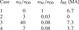
The radial profiles of the temperature, electric field and runaway current density at a few time slices are shown in figure 3 for Cases 2–4. In Case 2, shown in figure 3(a,d,g), the temperature remains of the order of  $100 \ \textrm {eV}$ in the central part of the plasma, resulting in very long CQ times. The increasing temperature in the central part of the plasma occurs because the injected material does not cause sufficient radiative losses to counteract the Ohmic heating there. Furthermore, due to the local temperature drop in the edge plasma, a strong electric field is induced (see figure 3d), and that will diffuse inward and lead to additional Ohmic heating. The effect of this increased heating is strongest close to the boundary between the hot and cold regions, where the electric field is induced, resulting in a radial peak also in the temperature. The resulting current evolution is shown as the solid curve in figure 4(a). After a rather fast drop initially while the current in the cold region decays, the CQ time for the remaining Ohmic current in the hot region is very slow. Notably, the runaway current remains negligibly small throughout the entire process.

Figure 3. Time slices from the temperature (a–c), the electric field (d–f) and the runaway current density (g–i) evolution. Left column (Case 2):  $n_\textrm {Ne}=3\times 10^{18}\ \textrm {m}^{-3}$, $n_\textrm {D}=3\times 10^{20}\ \textrm {m}^{-3}$ (very long CQ time). Middle column (Case 3): $n_\textrm {Ne}=8\times 10^{18}\ \textrm {m}^{-3}$, $n_\textrm {D}=4\times 10^{21}\ \textrm {m}^{-3}$ (low temperature and high runaway conversion). Right column (Case 4): $n_\textrm {Ne}=8\times 10^{18}\ \textrm {m}^{-3}$, $n_\textrm {D}=7\times 10^{20}\ \textrm {m}^{-3}$ (moderate runaway conversion).
Figure 4. (a) Current evolution. Thin black:  $I_\textrm {p}$; thick blue: $I_\textrm {RE}$. Solid: Case 2, $n_\textrm {Ne}=3\times 10^{18}\ \textrm {m}^{-3}$, $n_\textrm {D}=3\times 10^{20}\ \textrm {m}^{-3}$ (too long CQ time); dashed: Case 3, $n_\textrm {Ne}=8\times 10^{18}\ \textrm {m}^{-3}$, $n_\textrm {D}=4\times 10^{21}\ \textrm {m}^{-3}$ (low temperature and high runaway conversion); dash-dotted: Case 4, $n_\textrm {Ne}=8\times 10^{18}\ \textrm {m}^{-3}$, $n_\textrm {D}=7\times 10^{20}\ \textrm {m}^{-3}$ (lowest runaway fraction). (b) Current density profiles. Thin black line is $j_\|(t=0)$; thick blue lines represent $j_\textrm {RE}$ at the time of highest $I_\textrm {RE}$. Dashed: Case 3; dash-dotted: Case 4.
In Case 3 (high injected deuterium density), on the other hand, the radiative losses are strong, resulting in very low temperatures, which leads to a large runaway current, and a full current conversion. The temperature evolution for this case is presented in figure 3(b). The plasma is divided in two regions: an inner, continuously shrinking region with a temperature of  ${\sim }5\ \textrm {eV}$, and an outer region with a temperature as low as ${\sim }1\ \textrm {eV}$. The boundary between these two regions moves radially inward as the electric field decays away, and the heating decreases (compare figure 3(b) and 3(e)). In this case, however, radiative losses are strong enough to maintain a low temperature in the outer region, even when the electric field is sufficiently high to cause a significant runaway avalanche in part of the cold region.
At  $1\ \textrm {eV}$, the ionization degree of deuterium is significantly affected, so that a sizable fraction of the deuterium becomes neutral in the outer region of the plasma, as shown in figure 5. This strongly enhances the avalanche, due to the reduction in the free electron density. This enhancement makes the avalanche generation stronger in the outer part of the plasma, even if the electric field is lower there compared to the inner part. The result is a large runaway current of ${\sim }7.3\ \textrm {MA}$, with an off-axis maximum, the evolution of which is shown in figure 3(h), and the final current density profile is shown by the dashed line in figure 4(b). There is, however, a significant current dissipation due to the large effective critical electric field, such that by the end of the $150\ \textrm {ms}$ long simulation the remaining runaway current is only $3.2\ \textrm {MA}$.

Figure 5. Average ion charge as a function of radius for (a) neon and (b) deuterium for Case 3 ( $n_\textrm {Ne}=8\times 10^{18}\ \textrm {m}^{-3}$, $n_\textrm {D}=4\times 10^{21}\ \textrm {m}^{-3}$).
Finally, Case 4, representing an intermediate case between Case 1 and Case 3, has the lowest conversion, while also an acceptable CQ time. As can be seen in figure 3(c), the deuterium density is not high enough to result in sufficiently low temperatures to make the deuterium recombine, except close to the edge where the heating and the electric field are very low, but it is sufficiently high to dampen the avalanche, at least partially. The resulting runaway current evolution is shown in figure 3(i) and the total current evolution is shown by the dash-dotted line in figure 4(a). The final runaway current is  ${\sim }3.7\ \textrm {MA}$ with a radial profile centred near the magnetic axis (see figure 4(b)). The dissipation rate is relatively small with $\sim$13 % dissipation within the simulation time of $150\ \textrm {ms}$.
A limitation of the model used in this paper is that transport of neutral particles is not taken into account. Since the neutral particles are not confined by the magnetic field, they might be lost before giving rise to a significant enhancement of the avalanche. However, if a large fraction of the injected deuterium would recombine and leave the plasma, its contribution to the increase in the critical electric field would also be lost. Therefore the resulting runaway current turns out to be similar to a case with a lower amount of injected deuterium. Simulations, where neutral particles are instantaneously removed from the system, show that the runaway current for injected densities in the region around Case 3 is still as large as  $3$–
$3$– $4\ \textrm {MA}$, only a few percent of which is dissipated within the simulation time of $150\ \textrm {ms}$.
3.3 Qualitative analysis
The dynamics described in the four cases can be qualitatively understood by considering the behaviour of the avalanche growth rate, together with the balance between radiative losses and Ohmic heating, while assuming an equilibrium distribution over charge states. In figure 6, the radiative losses, the sum of radiative and ionization losses and the Ohmic heating are shown as functions of temperature, for the neon and deuterium densities of the four cases presented above. The Ohmic heating is shown for  $j_\textrm {ohm}=1.69\ \textrm {MA}\,\textrm {m}^{-2}$, corresponding to the initial on-axis current density, and for $j_\textrm {ohm}=0.2\ \textrm {MA}\,\textrm {m}^{-2}$, representing a case where the Ohmic current has partially, but not completely, decayed.
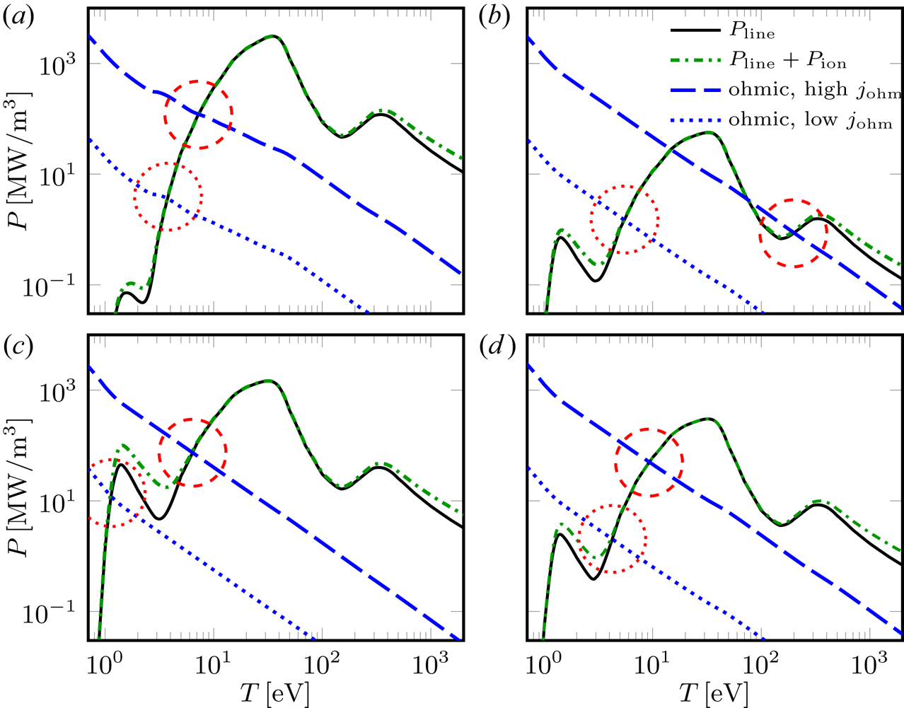
Figure 6. Radiative losses (solid), radiative and ionization losses (dash-dotted) and Ohmic heating (dashed and dotted) as functions of temperature for Case 1 (a), Case 2 (b), Case 3 (c) and Case 4 (d), assuming the equilibrium distribution over charge states. The Ohmic heating is shown for  $j_\textrm {ohm}=1.69\ \textrm {MA}\,\textrm {m}^{-2}$ (dashed) and $j_\textrm {ohm}=0.2\ \textrm {MA}\,\textrm {m}^{-2}$ (dotted); the corresponding stable equilibrium points are marked with circles.
In Case 1, shown in figure 6(a), the equilibrium temperatures for both current densities are of the order of a few  $\rm eV$. The avalanche growth rate is enhanced by the presence of a relatively large density of partially ionized neon. Therefore, this case results in a large RE conversion.
In Case 2, on the other hand, there is an equilibrium temperature at  ${\sim }200\ \textrm {eV}$ when $j_\textrm {ohm}=1.69\ \textrm {MA}\,\textrm {m}^{-2}$, as shown in figure 6(b). There is also an equilibrium at a lower temperature for this current density. However, since the Ohmic heating is stronger than the radiation losses at the central temperature of ${\sim }100 \ \textrm {eV}$ in the beginning of the simulation, where the losses are dominated by radiation, the temperature will increase towards the higher equilibrium. This mechanism causes the inner part of the plasma to remain hot, as observed in figure 3(a), and is responsible for the very long CQ time. Due to the high temperature, and thus high conductivity, the induced electric field is weak, and the corresponding avalanche growth rate is practically zero; thus RE conversion remains negligible.
With  $j_\textrm {ohm}=0.2 \ \textrm {MA}\,\textrm {m}^{-2}$, the (unique) equilibrium temperature shown in figure 6(b) is still of the order of a few $\rm eV$, corresponding to the cold, outer part of the plasma shown in figure 3(a). However, the induced electric field remains modest and the low amount of partially ionized material makes the avalanche growth rate – for a given electric field – small, which results in a small runaway generation rate even in this region.
In Case 3, figure 6(c) shows that the large amount of deuterium leads to an overall enhancement of the radiative losses. For  $j_\textrm {ohm}=0.2\ \textrm {MA}\,\textrm {m}^{-2}$, this shifts the equilibrium temperature from a few $\rm eV$ down to only ${\sim }1\ \textrm {eV}$, which corresponds to the cold outer part of the plasma in figure 3(c). This large reduction in the temperature makes a significant difference, as at this temperature the equilibrium degree of ionization of deuterium is only a few per cent. The presence of neutral deuterium enhances the avalanche growth rate, and the low temperature also favours an increased induced electric field. These circumstances result in a large avalanche generation in the outer part of the plasma in Case 3, even if the avalanche is partly constrained by a short CQ time and saturation effects. Note, however, that although the Ohmic current density is modest in this region, the Ohmic current remaining in the more central part of the plasma will have to pass through the cold region as it diffuses outwards. Therefore, a significant induced electric field is sustained in the cold region, and thus the local conversion is not limited by the local current density. The result is a large runaway current with an off-axis radial profile, as shown by the dashed line in figure 4(b).
Finally, Case 4 can be regarded as a compromise between the various features in the other three cases. The injected densities are sufficiently large to avoid an equilibrium at high temperatures (over  $100\ \textrm {eV}$), but not too large, such that equilibrium temperature does not drop too close to $1\ \textrm {eV}$ (unless the Ohmic current density is very low). This ensures an acceptably short CQ time, while still not leading to a large induced electric field. The ratio of the fully ionized deuterium and the partially ionized neon is large enough to limit partial screening effects on the avalanche growth rate, which contributes to the resulting runaway current remaining modest.
4 Discussion
When partially ionized impurities are introduced into the plasma, there are two competing effects which affect the avalanche growth rate: (1) additional target electrons become available for avalanche multiplication (represented by the prefactor  $n_\textrm {e}^\textrm {tot}$ in the growth rate formula (2.8)), which leads to an increasing growth rate; and (2) the critical runaway momentum $p_\star$ increases due to the enhancement of the collisional slowing-down and pitch-angle scattering processes (i.e. through increasing $\nu _\textrm {s}$ and $\nu _\textrm {D}$, respectively), which leads to a decreasing growth rate. For the scenarios considered here, we generally find that the additional-target effect prevails, leading to a net increased growth rate in the presence of impurity injection.
Our results predict a higher runaway conversion in the presence of MMI than previous estimates by Martín-Solís et al. (Reference Martín-Solís, Loarte and Lehnen2017). One of the reasons for the difference is that the avalanche growth rate is different in the two cases, mainly because the corrections to the slowing-down and deflection frequencies,  $\nu _\textrm {s}$ and $\nu _\textrm {D}$, due to partial screening are different; namely, Martín-Solís et al. (Reference Martín-Solís, Loarte and Lehnen2017) employs a fully classical model (Mosher Reference Mosher1975), whereas we take a quantum mechanical approach to determine the collision rates. Also, the expressions for the avalanche growth rates are slightly different. The growth rate used here, given in (2.8), is based on the calculation by Hesslow et al. (Reference Hesslow, Embréus, Vallhagen and Fülöp2019a), where analytical solutions of the kinetic equation were derived in the same parameter regimes as the Rosenbluth–Putvinski calculation, and benchmarked to kinetic simulations. In contrast, Martín-Solís, Loarte & Lehnen (Reference Martín-Solís, Loarte and Lehnen2015) consider an expression for the growth rate which is obtained in the momentum-diffusion-free limit, given in (21) of Martín-Solís et al. (Reference Martín-Solís, Loarte and Lehnen2015) as
 \begin{equation} \varGamma \equiv \frac{1}{ n_\textrm{RE}}\left(\frac{\partial n_\textrm{RE}}{\partial t}\right)_\textrm{aval}^{\rm MS}=\frac{2{\rm \pi} r_0^2 n_\textrm{e}^\textrm{tot} c }{\sqrt{1+(p_\star^\textrm{MS}/m_\textrm{e}c)^2}-1}, \end{equation}
where  $r_0$ is the classical electron radius, which would agree with our expression in the non-relativistic limit $p_\star \ll m_\textrm {e} c$, if $p_\star ^\textrm {MS}$ had been defined in the same way. Although it is not presented in this form, (16) of Martín-Solís et al. (Reference Martín-Solís, Loarte and Lehnen2015) defines the effective critical momentum as
 \begin{equation} eE_\parallel = \sqrt{p_\star^2\nu_\textrm{s}^\textrm{MS}(p_\star)[\nu_\textrm{D}^\textrm{MS}(p_\star)+\nu_\textrm{s}^\textrm{MS}(p_\star)]}, \end{equation}
which is similar to our result (2.3), but differs by the appearance of an additional  $\nu _\textrm {s}$ term and by the use of different collision frequencies. The choice of critical momentum leads to minor differences in the tritium seed current (see table 2). Our simulations show that the main difference between the results is not due to the difference between (4.1) and (2.8), but rather due to the choice of model for $\nu _\textrm {s}$ and $\nu _\textrm {D}$.
Table II. Seed currents ( $I_\textrm {seed}$) and final runaway currents ( $I_\textrm {RE}$) for combined argon and deuterium injection. $I_\textrm {seed}$: comparison between results using (4.2) and (2.3) with constant temperature. $I_\textrm {RE}$: comparison between results using avalanche growth rate expressions from (2.8) and (4.1) and different assumptions for temperature evolution (constant, time-dependent (2.11) or equilibrium (2.13)). $I_\textrm {RE}$ calculated using the assumptions used in Martín-Solís et al. (Reference Martín-Solís, Loarte and Lehnen2017) (avalanche growth rate from (4.1), $p_\star$ from (4.2) and constant temperature) agrees with the runaway currents obtained there. Seed runaways are assumed to originate only from tritium decay in all cases, and $p_\star$ from (2.3) is used in the last three columns.
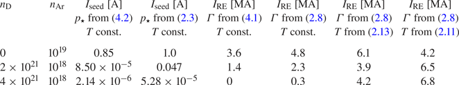
The other major difference is that here, the spatio-temporal evolution of the temperature is taken into account, while it was assumed to be constant in Martín-Solís et al. (Reference Martín-Solís, Loarte and Lehnen2017). As we have seen in the previous section, the evolution of the temperature has a crucial impact on the runaway dynamics. To quantify the differences, we have performed simulations for three different combinations of argon and deuterium injection, and compared the maximum runaway current values for various levels of sophistication of the modelling; the results are presented in table 2.
When we use the same avalanche growth rate as Martín-Solís et al. (Reference Martín-Solís, Loarte and Lehnen2017), and a constant temperature, we find agreement with their results. In particular, at sufficiently high deuterium injection the generation of runaways is completely suppressed. However, if the temperature evolution is included, we find a significant runaway conversion. At a fixed value of  $n_\textrm {Ar}$, the runaway conversion even increases upon an increasing amount of injected deuterium, when using (2.8). Furthermore, at high deuterium densities, determining the temperature evolution from the more accurate (2.11), rather than (2.13), leads to a further increase in the predicted runaway currents. Note that the radiation peak resulting from deuterium between 1 and 2 eV, that can be seen in figure 6(c), has not been taken into account in previous work.
The most interesting aspect of the cooling in connection with major quantities of deuterium is the partial recombination of the deuterium due to the low temperatures. In this case,  $n_\textrm {e}^\textrm {tot}/n_\textrm {e}$ increases, and the screened avalanche model predicts a significantly higher avalanche growth rate for a given electric field than in the fully ionized case. The reduced ionization degree of deuterium also impacts the conductivity, as discussed in appendix B: at $1\ \textrm {eV}$ the conductivity is reduced by 30 % compared to the Spitzer conductivity. However, simulations with this effect included show only a slightly higher runaway current, since the decrease in conductivity is counterbalanced by an increase in the induced electric field. This balance is further adjusted as the temperature also slightly increases due to a more efficient Ohmic heating for a given Ohmic current density.
So far all density profiles have been assumed to be flat. To test the sensitivity of the final runaway current to a radial variation of the density, we performed a series of simulations (not shown here) with density profiles varying from hollow to peaked. Through the four cases considered in the paper, we have divided the parameter space into four characteristic regions in terms of the runaway dynamics. We find that, as long as the radial density variation is not so strong that different parts of the plasma would correspond to different regions in this taxonomy, both the total runaway current and the CQ time are fairly insensitive to the radial density variation. While the radial density profile does affect the runaway current profile, as long as the total number of injected atoms are held constant, the total runaway current remains largely unaffected. A similar statement can be made regarding CQ time: the current decay rate may increase in some region and decrease in another, but total CQ time is only weakly affected. If, however, the radial density variation would become so strong that different parts of the plasma would correspond to different regions in our classification, effects characteristic of those regions could come into play simultaneously.
To assess the importance of a remnant hot-tail seed, we calculate the maximum runaway current as a function of seed current, assuming a flat seed profile for simplicity. Figure 7 shows the maximum runaway current as a function of seed current, for three of the cases we considered (Cases 1, 3 and 4). The final runaway current is approximately logarithmically sensitive to the seed. The reason for this weak dependence is that when the runaway current becomes comparable to the Ohmic current, the electric field is reduced, which reduces the avalanche growth rate. In the 15 MA case, shown in figure 7(a), as long as the seed current is above  $1\ \mathrm {\mu }$A (corresponding to a seed RE density of less than 2000 $\rm m^{-3}$) it results in more than 1 MA final runaway current even in the most optimistic Case 4. For a seed current of $1\ \mathrm {\mu }$A, Cases 1 and 3 lead to 4.7 and 5.2 MA, respectively.

Figure 7. Maximum runaway current as a function of seed current for Cases 1, 3 and 4, assuming a flat seed runaway profile. Initial plasma current is (a) 15 MA and (b) 10 MA.
In the absence of tritium decay and Compton sources, hot-tail generation is the only source that can give a significant runaway in the initial, non-nuclear operational phase of ITER. Simulations with only Dreicer source for a 10 MA ITER scenario show that, apart from rare cases when a filamentation of the temperature profile occurs where a substantial Dreicer seed can be generated, the seed current is extremely small (of the order of  $10^{-10}\ \textrm {A}$). As a result, the total runaway current is much less than $1$ MA except for deuterium densities high enough to cause a substantial recombination. However, as figure 7(b) shows, if there is a remnant hot-tail seed of the order of 0.5 A, it will result in large runaway currents also in the 10 MA scenario (3.7 MA for Case 1, 4.3 MA for Case 3 and 1.7 MA for Case 4). Note that hot-tail electrons are produced under a short period during the TQ, and if they are eliminated, they will not be reconstituted. In contrast, the tritium-decay and Compton-scattering seeds that are important in the DT phase are produced over a longer period of time and radial losses that occur only during the TQ are not sufficient for their deconfinement.
In this paper, the plasma was assumed to be transparent to radiative losses. However, plasmas at low temperature and high density (such as Case 3) are partly opaque to the Lyman lines of hydrogen isotopes. Not only is the energy balance changed due to the radiation being trapped in the plasma, but also the ionization and recombination rates (Pshenov et al. Reference Pshenov, Kukushkin, Marenkov and Krasheninnikov2019). The importance of opacity effects for runaway generation in the presence of low- $Z$ impurities such as beryllium and carbon has also been pointed out by Lukash, Mineev & Morozov (Reference Lukash, Mineev and Morozov2007). A proper treatment of the problem requires solution of radiation transport equations, which is outside the scope of the present paper. However, we can estimate an upper bound for the effect of opacity by considering the extreme case, when all the deuterium radiation is trapped in the plasma. The temperature is then determined from the energy balance equation (2.11), in which the deuterium line radiation is removed, along with the radiation corresponding to the ionization ( $P_\textrm {ion}$). The latter term is important in Case 3, as shown in figure 6 (note the difference between solid and dash-dotted lines close to the left radiation peak). Simulation results show that if only the deuterium line radiation is trapped (i.e. removed from (2.11)), the final runaway current is reduced from $7.3 \ \textrm {MA}$ (in the case of a fully transparent plasma) to $6\ \textrm {MA}$. If we also remove all the ionization radiation in (2.11), the final runaway current is reduced to $2.73\ \textrm {MA}$.
If we furthermore take into account the effect of opacity on the charge states, i.e. we use the ionization rates from the AMJUEL databaseFootnote 4 for the case when all Lyman radiation is blocked in (2.12), we find that recombination takes place at lower temperatures compared to the fully transparent case. The deuterium radiation losses are then lower and the corresponding radiation peak is moved to lower temperatures. If line radiation losses from neutral deuterium are removed from (2.11), the final runaway current becomes  $2.78\ \textrm {MA}$, which is only slightly larger than the $2.73\ \textrm {MA}$ obtained when both deuterium line radiation and ionization losses are removed.
In conclusion, our estimates suggest that opacity effects can lead to significantly lower (but still substantial) final runaway currents in the case of massive deuterium injection, and should therefore be subject to further investigation.
5 Conclusions
Simulations of plasma shutdown scenarios indicate that impurity injection can lead to high runaway currents in ITER. The dependence of the avalanche generation on the density of partially ionized species makes the runaway dynamics sensitive to the evolution of the temperature and the distribution of ionization states. Injection of large quantities of impurity and deuterium results also in a large runaway current due to the increased avalanche generation when deuterium recombines. On the other hand, a scenario with reduced runaway generation was identified numerically (Case 4), for moderate amounts of impurity and deuterium injection.
Potentially important effects that are not included in this study are hot-tail generation and loss processes due to magnetic perturbations, kinetic or MHD instabilities. The amount of runaway current deposited on plasma-facing components will depend on how large a fraction of the runaway current can be dissipated before eventually losing the runaway beam to the wall, which, in turn, depends on the effect of magnetic perturbations and on how long the runaway beam can be kept stable. Thus, the effects of transport phenomena, including the transport of neutral particles and radiation, are outstanding issues, requiring further investigation.
Appendix A. Critical momentum for runaway acceleration
The critical momentum for runaway generation is sometimes determined by setting the force balance to zero. However, this requires either that pitch-angle scattering is negligible, or that the pitch-angle distribution can be calculated analytically such as in Aleynikov & Breizman (Reference Aleynikov and Breizman2015), which is valid for electric fields near the threshold. In the case of strong electric fields and high plasma charge, the calculation of the avalanche growth rate by Rosenbluth & Putvinski (Reference Rosenbluth and Putvinski1997) can be extended to provide a threshold momentum for runaway acceleration that is valid for an arbitrary source function, following the same method as used in Hesslow et al. (Reference Hesslow, Embréus, Vallhagen and Fülöp2019a). In this approach, which we outline below, a solution of the kinetic equation provides an energy-dependent runaway probability, which sharply transitions from zero to unity near a momentum  $p_\star$ that we define as the critical momentum.
The kinetic equation in the superthermal limit can be written as
 \begin{align} \frac{\partial f}{\partial t} + eE_\parallel\left(\xi\frac{\partial f}{\partial p} + \frac{1-\xi^2}{p}\frac{\partial f}{\partial \xi}\right) = \frac{1}{p^2}\frac{\partial}{\partial p}(p^3\nu_\textrm{s} f) + \frac{\nu_\textrm{D}}{2}\frac{\partial}{\partial \xi}\left[(1-\xi^2)\frac{\partial f}{\partial \xi}\right] + S(p, \xi), \end{align}
where  $\xi =p_\|/p$, with the momentum component parallel to the magnetic field $p_\|$, and $S$ denotes an arbitrary particle source. We solve (A 1) perturbatively in the limit of strong pitch angle scattering and strong electric fields by ordering $\nu _\textrm {D} \sim \delta ^0$, $eE \sim \delta$, $\nu _\textrm {s} \sim S \sim \delta ^2$ and $\partial /\partial t \sim \delta ^3$. Then, writing $f=f_0+\delta f_1+\delta ^2 f_2 + \cdots$, we obtain the system of equations
 \begin{gather} \frac{\partial}{\partial \xi}\left[(1-\xi^2)\frac{\partial f_0}{\partial \xi}\right] = 0, \end{gather}
 \begin{gather}eE_\parallel \left(\xi\frac{\partial f_0}{\partial p} + \frac{1-\xi^2}{p}\frac{\partial f_0}{\partial \xi}\right) = \frac{\nu_\textrm{D}}{2}\frac{\partial}{\partial \xi}\left[(1-\xi^2)\frac{\partial f_1}{\partial \xi}\right], \end{gather}
 \begin{gather}eE_\parallel \left(\xi\frac{\partial f_1}{\partial p} + \frac{1-\xi^2}{p}\frac{\partial f_1}{\partial \xi}\right) = \frac{1}{p^2}\frac{\partial}{\partial p}\Big(p^3 \nu_\textrm{s}f_0\Big) + \frac{\nu_\textrm{D}}{2}\frac{\partial}{\partial \xi}\left[(1-\xi^2)\frac{\partial f_2}{\partial \xi}\right] + S(p,\xi). \end{gather}
The first equation yields the general solution
 \begin{equation} f_0 = f_0(t,p), \end{equation}
i.e. the leading-order distribution is isotropic, upon which the second equation takes the form
 \begin{equation} \left. \begin{array}{c@{}} \dfrac{2e E_\parallel}{\nu_\textrm{D} }\xi\dfrac{\partial f_0}{\partial p } =\dfrac{\partial}{\partial \xi}\left[(1-\xi^2)\dfrac{\partial f_1}{\partial \xi}\right], \\ \Rightarrow f_1 = -\xi \dfrac{eE_\parallel}{\nu_\textrm{D} } \dfrac{\partial f_0}{\partial p}. \end{array}\right\} \end{equation}
Integrating the third equation over  $\xi$ from $-$1 to 1 and inserting this solution for $f_1$ yields
 \begin{equation} - \frac{1}{p^2}\frac{\partial}{\partial p} \left[ p^2\left( \frac{{e}^2 E_\parallel^2}{3\nu_\textrm{D} }\frac{\partial f_0}{\partial p} + p\nu_\textrm{s} f_0 \right)\right] = \frac{1}{2}\int_{-1}^1 S\,{\textrm{d}} \xi,\end{equation}
from which we can derive the critical momentum,  $p_\star$, as follows. The runaway generation rate $\partial n_\textrm {RE}/\partial t$ can be defined as the particle flux to infinity, which, if we compare (A 7) with the initial kinetic equation, can be written
 \begin{equation} \frac{\partial n_\textrm{RE}}{\partial t} = -4{\rm \pi} p^2\left(\frac{{e}^2 E_\parallel^2}{3\nu_\textrm{s}}\frac{\partial f_0}{\partial p} + p\nu_\textrm{s} f_0\right)_{p=\infty}. \end{equation}
Therefore, if we multiply (A 7) by  $p^2$ and integrate over all momenta, we obtain
 \begin{equation} p^2\frac{{e}^2E_\parallel^2}{3\nu_\textrm{D}}\frac{\partial f_0}{\partial p} + p^3\nu_\textrm{s} f_0 = -\frac{1}{4{\rm \pi}}\frac{\partial n_\textrm{RE}}{\partial t} + \frac{1}{2} \int_p^\infty \,{\textrm{d}} p^{\prime} p^{\prime2} \int_{-1}^1 \,{\textrm{d}} \xi S(p^{\prime},\xi). \end{equation}
This first-order linear ordinary differential equation can be solved by introducing an integrating factor  $G$
$G$
 \begin{equation} G(p) = -\int_p^\infty \frac{3p^{\prime}\nu_\textrm{s} \nu_\textrm{D}}{{e}^2 E_\parallel^2} \,{\textrm{d}} p^{\prime}, \end{equation}
upon which the equation takes the form
 \begin{equation} \frac{\partial}{\partial p}( \textrm{e}^{G(p)}f_0(p) ) = \frac{3\nu_\textrm{D} \textrm{e}^{G(p)}}{p^2 {e}^2 E_\parallel^2}\left(- \frac{1}{4{\rm \pi}}\frac{\partial n_\textrm{RE}}{\partial t} + \frac{1}{2} \int_p^\infty \,{\textrm{d}} p^{\prime} p^{\prime2}\int_{-1}^1 \,{\textrm{d}} \xi S(p^{\prime},\xi)\right). \end{equation}
Since  $p \nu _\textrm {s}\nu _\textrm {D} \propto 1/p^5$ for small momenta, $G \propto -1/p^4$ for $p\to 0$. Then, if we integrate this equation over $p$ from $0$ to $\infty$ and assume that $f_0$ is well-behaved (i.e. is finite at the origin and vanishes at infinity), we obtain
 \begin{align} \frac{\partial n_\textrm{RE}}{\partial t} \int_0^\infty \frac{3\nu_\textrm{D} \,\textrm{e}^G}{p^2 {e}^2E_\parallel^2} \,{\textrm{d}} p &= \int_0^\infty \,{\textrm{d}} p \frac{3\nu_\textrm{D} \,\textrm{e}^G}{p^2 {e}^2E_\parallel^2} 2{\rm \pi} \int_p^\infty \,{\textrm{d}} p' p'^2 \int_{-1}^1\,{\textrm{d}} \xi S(p',\xi) \nonumber\\ &= 2{\rm \pi}\int_0^\infty \,{\textrm{d}} p p^2\int_{-1}^1 \,{\textrm{d}} \xi S(p,\xi) \int_0^p\,{\textrm{d}} p' \frac{3\nu_\textrm{D}(p') \,\textrm{e}^{G(p')}}{p'^2 {e}^2E_\parallel^2}, \end{align}
where in the second line we exchanged integration orders of  $p'$ and $p$. From this, it follows that the runaway generation rate due to an arbitrary source function takes the form
 \begin{equation} \left.\begin{array}{c@{}} \displaystyle\dfrac{\partial n_\textrm{RE}}{\partial t} = \int S(\boldsymbol{p}) h(p) \,{\textrm{d}}\boldsymbol{p},\\ h(p) = \dfrac{\displaystyle\int_0^p\,{\textrm{d}} p' \dfrac{3\nu_\textrm{D}(p') \,\textrm{e}^{G(p')}}{p'^2 {e}^2E_\parallel^2}}{ \displaystyle\int_0^\infty \,{\textrm{d}} p' \,\dfrac{3\nu_\textrm{D}(p') \,\textrm{e}^{G(p')}}{p'^2 {e}^2E_\parallel^2}}. \end{array}\right\} \end{equation}
Note that this equation is valid for a source term with an arbitrary pitch angle dependence and is valid for non-relativistic as well as relativistic energies. Since  $\nu _\textrm {s}$ and $\nu _\textrm {D}$ are monotonically decreasing functions, the function $h(p)$ will be monotonically increasing from $h(0) = 0$ to $h(\infty ) = 1$, and can therefore be interpreted as the runaway probability function for an electron born at $p$ to reach arbitrarily large momenta.
Since the function  $G(p)$ varies very rapidly with $p$ – approximately as $-1/p^4$ – the function $h$ will make a sharp transition from essentially $0$ to $1$ in the momentum region where $G$ crosses $-1$. This can be readily confirmed for an ideal non-relativistic plasma with $\nu _\textrm {s}, \nu _\textrm {D} \propto 1/p^3$, for which we can obtain the exact result $h(p) = \exp [G(p)] = \exp \{-3(1+Z)/[4(E/E_{c})^2p^4]\}$.
Therefore, we may approximate  $h(p)$ as a step function $h=\varTheta (p-p_\star )$, where we define $p_\star$ via
 \begin{equation} \left.\begin{array}{c@{}} G(p_\star) = -1, \\ p_\star^2 \approx \sqrt{\dfrac{3}{4}} \dfrac{E_\parallel/E_{c}}{\sqrt{\bar\nu_\textrm{s}(p_\star)\bar\nu_\textrm{D}(p_\star)}} \quad \text{(non-relativistic)}. \end{array}\right\} \end{equation}
The factor  $\sqrt {3/4}$ is not significant and has been neglected in this paper. Interestingly, the expression for $p_\star$ is the same as the one appearing in the avalanche formula, which was interpreted as an effective momentum for runaway acceleration.
Appendix B. Spitzer conductivity in weakly ionized plasmas
When the temperature in a plasma consisting mainly of deuterium becomes as low as  $1\ \textrm {eV}$, the ionization fraction falls to a few per cent, as shown in figure 5. Then the effect of electron–neutral collisions on the conductivity has to be taken into account.
The conductivity in a very weakly ionized plasma, where electron–neutral collisions dominate, is given by Nighan (Reference Nighan1969) as
 \begin{equation} \sigma=-\frac{4{\rm \pi}}{3}\frac{{e}^2}{m_\textrm{e}}\int_0^\infty \frac{1}{\nu_\textrm{en}(v)} \frac{\partial f_0}{\partial v}v^3\, \mathrm{d}v, \end{equation}
where  $f_0$ denotes the Maxwell distribution of electrons and $\nu _\textrm {en}(v)=n_\textrm {n}Q_\textrm {en}(v)v$ is the electron–neutral collision frequency, with the density of neutral atoms $n_\textrm {n}$, the electron–neutral momentum exchange cross-section $Q_\textrm {en}=2{\rm \pi} \int _0^{{\rm \pi} }I(\theta ,v)[1-\cos {(\theta )}]\sin {(\theta )}\, \mathrm {d}\theta$ and the electron–neutral differential scattering cross-section $I(\theta , v)$.
If electron–electron collisions were negligible in a fully ionized plasma, the conductivity would take the same form as (B 1), but with  $\nu _\textrm {en}(v)$ replaced by the electron–ion collision frequency, $\nu _\textrm {ei}(v)=Z_\textrm {eff} ({e}^4 n_\textrm {e} \ln \varLambda_c )/(4 {\rm \pi}\epsilon _0^2 m_\textrm {e}^2 v^3)$. Furthermore, as shown by Spitzer & Härm (Reference Spitzer and Härm1953), when electron–electron collisions are accounted for, the conductivity in a fully ionized plasma with an effective ion charge $Z_\textrm {eff}=1$ differs from the result with electron–ion collisions only by a factor $\gamma _\textrm {E}=0.58$.
With these considerations, Nighan (Reference Nighan1969) constructed an approximate expression for the conductivity, which reproduces the fully ionized and the very weakly ionized limits, and provides a reasonably good approximation between:
 \begin{equation} \sigma=-\frac{4{\rm \pi}}{3}\frac{{e}^2}{m_\textrm{e}}\int_0^\infty \frac{1}{\gamma_\textrm{E}^{-1}\nu_\textrm{ei}(v)+\nu_\textrm{en}(v)}\frac{\partial f_0}{\partial v}v^3\, \mathrm{d}v. \end{equation}
 By writing  $\nu _\textrm {en}=\bar {\nu }_\textrm {en}x Q(x)/\bar {Q}$ and $\nu _\textrm {ei}=\bar {\nu }_\textrm {ei}/x^3$, where a bar denotes a value at the thermal velocity, and $x=v/v_\textrm {th}$, we can write (B 2) as
 \begin{equation} \sigma=\frac{\sigma_\textrm{Sp}}{3}\int_0^\infty\frac{x^4\, \textrm{e}^{-x^2}}{\gamma_\textrm{E} \dfrac{\bar{\nu}_\textrm{en}}{\bar{\nu}_\textrm{ei}}\dfrac{Q(x)}{\bar{Q}}x+\dfrac{1}{x^3}}\, \mathrm{d}x. \end{equation}
In our calculations we use (B 3) to compute the plasma conductivity, for which we obtain the momentum exchange electron–neutral collisional cross-section  $Q_\textrm {en}$ for neon and deuterium from Itikawa (Reference Itikawa1978). Furthermore, we use the value of $\gamma _\textrm {E}$ corresponding to $Z_\textrm {eff}=1$, since whenever the ionization degree becomes as low as to modify the conductivity significantly, the densities of the ionization states greater than 1 are low.
Figure 8 illustrates the reduction of the conductivity compared to the Spitzer value. The ionization degree for a given temperature is calculated assuming collisional–radiative equilibrium, i.e. by solving (2.14). This temperature is then used to calculate the collision frequencies  $\bar {\nu }_\textrm {en}$ and $\bar {\nu }_\textrm {ei}$, used in (B 3) to calculate $\sigma /\sigma _\textrm {Sp}$. While at a temperature as low as $1\ \textrm {eV}$ the deviation from the Spitzer conductivity is only $\sim$30 %, even if the ionization degree is as low as $\approx 5\,\%$, if the temperature is decreased further, $\sigma /\sigma _\textrm {Sp}$ drops quite rapidly. That the three different plasma compositions considered in figure 8 result in essentially identical results reflects that the ionization degree is only a weak function of deuterium density, and that a comparatively small fraction of neon has a negligible effect.

Figure 8. Electrical conductivity relative to its Spitzer value at collisional–radiative equilibrium as a function of temperature for various plasma compositions. Solid:  $n_\textrm {D}=10^{20} \ \textrm {m}^{-3}$; dashed: $n_\textrm {D}=10^{22} \ \textrm {m}^{-3}$; dotted: $n_\textrm {D}=4 \times 10^{21} \ \textrm {m}^{-3}$ and $n_\textrm {Ne}=8 \times 10^{18} \ \textrm {m}^{-3}$ (Case 3). Note that the curves corresponding to the three cases overlap.
Acknowledgements
The authors are grateful to S. Newton, G. Papp, M. Hoppe, E. Nardon, S. Krasheninnikov and A. Kukushkin for fruitful discussions. This work was supported by the Swedish Research Council (Dnr. 2018-03911), the European Research Council (ERC-2014-CoG grant 647121) and the EUROfusion – Theory and Advanced Simulation Coordination (E-TASC). The work has been carried out within the framework of the EUROfusion Consortium and has received funding from the Euratom research and training programme 2014–2018 and 2019–2020 under grant agreement no. 633053. The views and opinions expressed herein do not necessarily reflect those of the European Commission.
Editor Alex Robinson thanks the referees for their advice in evaluating this article.
Declaration of interests
The authors report no conflict of interest.


 Open access