


1 Introduction
Turbulent magnetic fields are ubiquitous in the universe and their role in determining energetic particle transport is key to understanding the confinement and acceleration of high-energy cosmic rays (Hall & Sturrock Reference Hall and Sturrock1967; Kulsrud Reference Kulsrud1995; Schekochihin & Cowley Reference Schekochihin and Cowley2006; Gregori, Reville & Miniati Reference Gregori, Reville and Miniati2015; Marcowith et al.
Reference Marcowith, Bret, Bykov, Dieckman, O’C Drury, Lembège, Lemoine, Morlino, Murphy and Pelletier2016). As particles traverse a turbulent, magnetised plasma, they undergo a random walk in both physical and momentum space. The latter process is referred to as second-order Fermi acceleration, being a generalisation of the mechanism proposed by Fermi (Reference Fermi1949). Fermi observed that repeated elastic scattering of fast particles off slow moving ‘magnetised clouds’, when averaged over a random distribution of cloud velocities, produce a net gain in energy. The rate of energy gain is slightly higher than the rate of energy loss because head-on collisions are more probable than overtaking ones, the net gain being proportional to
 $(u/v)^{2}$
where
$(u/v)^{2}$
where
 $u$
is the mean fluid velocity and
$u$
is the mean fluid velocity and
 $v(\gg u)$
the particle velocity. Subsequently the focus has shifted from discrete interactions with magnetised clouds to continuous scattering in magneto-hydrodynamic (MHD) turbulence, but the underlying principle remains the same. Fermi noted shortly afterwards that converging flows, such as might exist between galactic spiral arms, result in a faster first-order process where the energy gain is proportional to
$v(\gg u)$
the particle velocity. Subsequently the focus has shifted from discrete interactions with magnetised clouds to continuous scattering in magneto-hydrodynamic (MHD) turbulence, but the underlying principle remains the same. Fermi noted shortly afterwards that converging flows, such as might exist between galactic spiral arms, result in a faster first-order process where the energy gain is proportional to
 $u/v$
(Fermi Reference Fermi1954). Indeed first-order Fermi acceleration in the converging fluid flow of astrophysical shock waves is currently the preferred model for the origin of cosmic rays (Bell Reference Bell1978; Blandford & Ostriker Reference Blandford and Ostriker1978; Blandford & Eichler Reference Blandford and Eichler1987). However the second-order mechanism can be more efficient for accelerating non-relativistic thermal background plasma particles and under certain conditions can also preferentially accelerate electrons relative to protons, as is required to explain many astrophysical sources (Petrosian Reference Petrosian2012). In reality there may be a hybrid mechanism, e.g. initial second-order acceleration of background plasma particles by turbulence, followed by a second stage of first-order acceleration by a shock wave.
$u/v$
(Fermi Reference Fermi1954). Indeed first-order Fermi acceleration in the converging fluid flow of astrophysical shock waves is currently the preferred model for the origin of cosmic rays (Bell Reference Bell1978; Blandford & Ostriker Reference Blandford and Ostriker1978; Blandford & Eichler Reference Blandford and Eichler1987). However the second-order mechanism can be more efficient for accelerating non-relativistic thermal background plasma particles and under certain conditions can also preferentially accelerate electrons relative to protons, as is required to explain many astrophysical sources (Petrosian Reference Petrosian2012). In reality there may be a hybrid mechanism, e.g. initial second-order acceleration of background plasma particles by turbulence, followed by a second stage of first-order acceleration by a shock wave.
The second-order Fermi process is quite general, requiring only turbulent magnetised fluid motions and injection of particles with energy above that of the background thermal plasma. Relevant environments are common in the universe and stochastic acceleration is believed to be responsible for phenomena as diverse as e.g. radio emission from young supernova remnants entering the Sedov–Taylor phase (Cowsik & Sarkar Reference Cowsik and Sarkar1984), the ejection of mass from the solar corona (Nelson & Melrose Reference Nelson and Melrose1985), the acceleration of particles in the jets of active galactic nuclei and in their giant radio lobes (Tramacere, Massaro & Cavaliere Reference Tramacere, Massaro and Cavaliere2007; Hardcastle et al.
Reference Hardcastle, Cheung, Feain and Stawarz2009; O’Sullivan, Reville & Taylor Reference O’Sullivan, Reville and Taylor2009) and
 $\unicode[STIX]{x1D6FE}$
-ray emission from the Fermi bubbles (Mertsch & Sarkar Reference Mertsch and Sarkar2011).
$\unicode[STIX]{x1D6FE}$
-ray emission from the Fermi bubbles (Mertsch & Sarkar Reference Mertsch and Sarkar2011).
The necessary conditions may be accessible in laboratory experiments (Gregori et al. Reference Gregori, Reville and Miniati2015) thus providing a platform to explore particle acceleration in a controlled setting and isolate the effects of relevance to astrophysical models. We explore here the possibility of validating the physics of second-order Fermi acceleration using existing experimental set-ups (see supplementary material to Tzeferacos et al. (Reference Tzeferacos, Rigby, Bott, Bell, Bingham, Casner, Cattaneo, Churazov, Emig and Fiuza2018)). In § 2 we introduce the proposed set-up and place it in the context of previous experiments. The governing equations for the momentum-space diffusion process are stated in § 3 and the relevant Fokker–Planck coefficients of the diffusion process are estimated. We discuss the relevant time scales to justify the diffusion approach adopted. An analytic solution for the diffusion equation is investigated in § 4. Finally in § 5, laser experiments at the National Ignition Facility (NIF), Livermore, USA (Hogan et al. Reference Hogan, Moses, Warner, Sorem and Soures2001) are discussed. We conclude that the effects of stochastic Fermi acceleration are measurable in the laboratory.
2 Experimental set-up
Experiments with high power lasers have achieved conditions where strong magnetised turbulence can be sustained over large spatial scales and thus provide insights into the origin and amplification of magnetic fields in the intergalactic medium (Meinecke et al.
Reference Meinecke, Doyle, Miniati, Bell, Bingham, Crowston, Drake, Fatenejad, Koenig and Kuramitsu2014, Reference Meinecke, Tzeferacos, Bell, Bingham, Clarke, Churazov, Crowston, Doyle, Drake and Heathcote2015; Gregori et al.
Reference Gregori, Reville and Miniati2015). Tzeferacos et al. (Reference Tzeferacos, Rigby, Bott, Bell, Bingham, Casner, Cattaneo, Churazov, Emig and Fiuza2018) describe how a high power laser was used to generate two counter-streaming plasma flows from direct ablation of CH (plastic) foils. Each flow was guided through a grid of
 $300~\unicode[STIX]{x03BC}\text{m}$
holes with a
$300~\unicode[STIX]{x03BC}\text{m}$
holes with a
 $300~\unicode[STIX]{x03BC}\text{m}$
spacing between holes. The grids were spatially shifted to increase turbulent motions in the plasma and enhance the turbulent dynamo processes responsible for amplification of magnetic seed fields. This produced turbulent structures with an outer scale of
$300~\unicode[STIX]{x03BC}\text{m}$
spacing between holes. The grids were spatially shifted to increase turbulent motions in the plasma and enhance the turbulent dynamo processes responsible for amplification of magnetic seed fields. This produced turbulent structures with an outer scale of
 ${\sim}600~\unicode[STIX]{x03BC}\text{m}$
in the colliding region. These results were obtained using multi-kJ laser systems. At the NIF, a MJ of laser energy is available so more extreme conditions are to be expected, as shown in table 1. We adopt these estimated parameters in order to assess the feasibility of a ‘cosmic ray acceleration platform’ in the laboratory. The first step is the injection of cosmic ray particles, which can be implemented by replacing the CH foils used earlier (Tzeferacos et al.
Reference Tzeferacos, Rigby, Bott, Bell, Bingham, Casner, Cattaneo, Churazov, Emig and Fiuza2018) by CD (deuterated plastic) foils. Within the turbulent plasma region, 3 MeV protons (with velocity
${\sim}600~\unicode[STIX]{x03BC}\text{m}$
in the colliding region. These results were obtained using multi-kJ laser systems. At the NIF, a MJ of laser energy is available so more extreme conditions are to be expected, as shown in table 1. We adopt these estimated parameters in order to assess the feasibility of a ‘cosmic ray acceleration platform’ in the laboratory. The first step is the injection of cosmic ray particles, which can be implemented by replacing the CH foils used earlier (Tzeferacos et al.
Reference Tzeferacos, Rigby, Bott, Bell, Bingham, Casner, Cattaneo, Churazov, Emig and Fiuza2018) by CD (deuterated plastic) foils. Within the turbulent plasma region, 3 MeV protons (with velocity
 $v_{\text{p}}\sim 8\times 10^{-2}~\text{c}$
) will be produced via D–D collisions in the counter-streaming plasma flows (Ross et al.
Reference Ross, Higginson, Ryutov, Fiuza, Hatarik, Huntington, Kalantar, Link, Pollock and Remington2017). Analogous to the astrophysical situation, these protons, as they stream out from the plasma, interact with the turbulent magnetic fields and should be accelerated by the second-order Fermi process. We now model this interaction to predict the energy spectrum of the protons.
$v_{\text{p}}\sim 8\times 10^{-2}~\text{c}$
) will be produced via D–D collisions in the counter-streaming plasma flows (Ross et al.
Reference Ross, Higginson, Ryutov, Fiuza, Hatarik, Huntington, Kalantar, Link, Pollock and Remington2017). Analogous to the astrophysical situation, these protons, as they stream out from the plasma, interact with the turbulent magnetic fields and should be accelerated by the second-order Fermi process. We now model this interaction to predict the energy spectrum of the protons.
Table 1. The expected plasma parameters for the proposed experiment at the NIF, LLNL. These are derived from experiments done at other facilities (Tzeferacos et al. Reference Tzeferacos, Rigby, Bott, Bell, Bingham, Casner, Cattaneo, Churazov, Emig and Fiuza2018), rescaled to NIF laser drive conditions. The estimates for the Reynolds and magnetic Reynolds number follow Spitzer & Härm (Reference Spitzer and Härm1953) and Braginskii (Reference Braginskii1965). However, as discussed in Ryutov et al. (Reference Ryutov, Drake, Kane, Liang, Remington and Wood-Vasey1999), micro-instabilities may alter our estimates.

a The dependence on B is made explicit here, as we consider different values throughout the paper. All other parameters are as stated in table 1.
 $\unicode[STIX]{x1D6FD}=4\times 10^{-11}nT/B^{2}$
in Gaussian cgs.
$\unicode[STIX]{x1D6FD}=4\times 10^{-11}nT/B^{2}$
in Gaussian cgs.
As each scatter changes the energy of a particle by a small fraction of its initial energy, this is a diffusion process in momentum space described by a Fokker–Planck transport equation for
 $f(p,t)$
, the phase-space density of the protons in the plasma (Hall & Sturrock Reference Hall and Sturrock1967; Tverskoǐ Reference Tverskoǐ1967; Blandford & Eichler Reference Blandford and Eichler1987; Ostrowski & Siemieniec-Oziȩbło Reference Ostrowski and Siemieniec-Oziȩbło1997):
$f(p,t)$
, the phase-space density of the protons in the plasma (Hall & Sturrock Reference Hall and Sturrock1967; Tverskoǐ Reference Tverskoǐ1967; Blandford & Eichler Reference Blandford and Eichler1987; Ostrowski & Siemieniec-Oziȩbło Reference Ostrowski and Siemieniec-Oziȩbło1997):
 $$\begin{eqnarray}\left(\frac{\unicode[STIX]{x2202}f}{\unicode[STIX]{x2202}t}\right)_{\text{inner}}=\frac{1}{p^{2}}\frac{\unicode[STIX]{x2202}}{\unicode[STIX]{x2202}p}\left(p^{2}D_{p}\frac{\unicode[STIX]{x2202}f}{\unicode[STIX]{x2202}p}\right)-\frac{f}{\unicode[STIX]{x1D70F}_{\text{esc}}}+\frac{C_{0}\unicode[STIX]{x1D6FF}(p-p_{0})\unicode[STIX]{x1D6FF}(t-t_{0})}{4\unicode[STIX]{x03C0}p^{2}}.\end{eqnarray}$$
Here
 $D_{p}$
is the momentum diffusion coefficient,
$D_{p}$
is the momentum diffusion coefficient,
 $\unicode[STIX]{x1D70F}_{\text{esc}}$
the escape time describing the loss of protons from the system and the last term describes instantaneous injection of
$\unicode[STIX]{x1D70F}_{\text{esc}}$
the escape time describing the loss of protons from the system and the last term describes instantaneous injection of
 $C_{0}$
superthermal particles at time
$C_{0}$
superthermal particles at time
 $t_{0}$
and of momentum
$t_{0}$
and of momentum
 $p_{0}$
. Note that spatial homogeneity is assumed in writing down (2.1), however we will assume that the injection occurs only in the central region of the plasma. The particle distribution function
$p_{0}$
. Note that spatial homogeneity is assumed in writing down (2.1), however we will assume that the injection occurs only in the central region of the plasma. The particle distribution function
 $n$
is related to the phase-space density
$n$
is related to the phase-space density
 $f$
through
$f$
through
 $$\begin{eqnarray}n(p,t)=4\unicode[STIX]{x03C0}p^{2}f(p,t).\end{eqnarray}$$
The diffusion equation (2.2) has been solved for a variety of situations (Kaplan Reference Kaplan1956; Hall & Sturrock Reference Hall and Sturrock1967; Tverskoǐ Reference Tverskoǐ1967; Cowsik & Sarkar Reference Cowsik and Sarkar1984; Mertsch Reference Mertsch2011) and we discuss below the appropriate solution for the proposed experiment.
The detectors used to measure the proton energy are located outside the plasma, hence the relevant distribution function to consider is that of the escaping protons. This can be related to the particle distribution function of the protons inside the plasma by requiring that the proton number be conserved after the injection, i.e. at
 $t>t_{0}$
 $$\begin{eqnarray}\left(\frac{\unicode[STIX]{x2202}n}{\unicode[STIX]{x2202}t}\right)_{\text{outer}}=\frac{n_{\text{inner}}}{\unicode[STIX]{x1D70F}_{\text{esc}}},\end{eqnarray}$$
where
 $f_{\text{inner}}$
is the solution of (2.1). As will be shown in § 3, the escape time
$f_{\text{inner}}$
is the solution of (2.1). As will be shown in § 3, the escape time
 $\unicode[STIX]{x1D70F}_{\text{esc}}$
is momentum dependent, so the phase-space density inside and outside the plasma will be different.
$\unicode[STIX]{x1D70F}_{\text{esc}}$
is momentum dependent, so the phase-space density inside and outside the plasma will be different.
3 The transport coefficients
The Fokker–Planck transport coefficient for energy diffusion is (e.g. Blandford & Eichler Reference Blandford and Eichler1987)
 $$\begin{eqnarray}D_{\unicode[STIX]{x1D716}}=\frac{\langle (\unicode[STIX]{x0394}\unicode[STIX]{x1D716})^{2}\rangle }{\unicode[STIX]{x0394}t},\end{eqnarray}$$
where
 $\langle .\rangle$
denotes the average over scattering angles, and the energy change per scatter is given by the integral over the force exerted by the electric field fluctuations, i.e.
$\langle .\rangle$
denotes the average over scattering angles, and the energy change per scatter is given by the integral over the force exerted by the electric field fluctuations, i.e.
 $$\begin{eqnarray}\langle (\unicode[STIX]{x0394}\unicode[STIX]{x1D716})^{2}\rangle =\left\langle \left(e\int \boldsymbol{E}\boldsymbol{\cdot }\text{d}\boldsymbol{s}\right)^{2}\right\rangle \sim \text{e}^{2}\ell ^{2}\langle (E_{\Vert })^{2}\rangle .\end{eqnarray}$$
Here,
 $\boldsymbol{s}$
is the world line of the particle and
$\boldsymbol{s}$
is the world line of the particle and
 $\ell$
is the scale length of the turbulence cells in the plasma flow. These cells are defined by the scale on which the electric field,
$\ell$
is the scale length of the turbulence cells in the plasma flow. These cells are defined by the scale on which the electric field,
 $\boldsymbol{E}$
, is statistically de-correlated, close to the outer scale of the turbulent spectrum.
$\boldsymbol{E}$
, is statistically de-correlated, close to the outer scale of the turbulent spectrum.
The appropriate Ohm’s law reads:
 $$\begin{eqnarray}\boldsymbol{E}=-\frac{\boldsymbol{u}\times \boldsymbol{B}}{c}-\frac{\unicode[STIX]{x1D735}P_{\text{e}}}{ne},\end{eqnarray}$$
where
 $P_{e}$
is the isotropic electron pressure,
$P_{e}$
is the isotropic electron pressure,
 $n$
is the electron density and
$n$
is the electron density and
 $\boldsymbol{u}$
is the electron velocity field. In principle, Ohm’s law contains possible additional contributions but these turn out to be small in the present case as e.g. the Reynolds and magnetic Reynolds numbers are large. Note that the ratio of the two, the magnetic Prandtl number
$\boldsymbol{u}$
is the electron velocity field. In principle, Ohm’s law contains possible additional contributions but these turn out to be small in the present case as e.g. the Reynolds and magnetic Reynolds numbers are large. Note that the ratio of the two, the magnetic Prandtl number
 $P_{\text{m}}=R_{\text{m}}/Re$
, is much larger than unity at the NIF (see table 1), confirming that the plasma is in an astrophysically relevant regime.
$P_{\text{m}}=R_{\text{m}}/Re$
, is much larger than unity at the NIF (see table 1), confirming that the plasma is in an astrophysically relevant regime.
For the assumed conditions at the NIF, the pressure term is insignificant, being of
 $O(10^{-2})$
. We will retain it nevertheless as it is relevant for conditions achievable at other facilities such as OMEGA (Boehly et al.
Reference Boehly, Brown, Craxton, Keck, Knauer, Kelly, Kessler, Kumpan, Loucks and Letzring1997).
$O(10^{-2})$
. We will retain it nevertheless as it is relevant for conditions achievable at other facilities such as OMEGA (Boehly et al.
Reference Boehly, Brown, Craxton, Keck, Knauer, Kelly, Kessler, Kumpan, Loucks and Letzring1997).
Returning to the Fokker–Planck transport coefficient (3.1), we find by combining (3.2) and (3.3)
 $$\begin{eqnarray}\displaystyle \langle (\unicode[STIX]{x0394}\unicode[STIX]{x1D716})^{2}\rangle & = & \displaystyle \text{e}^{2}\ell ^{2}\left\langle \left(\frac{u^{2}B^{2}}{c^{2}}\sin ^{2}(\unicode[STIX]{x1D703})\right)\right\rangle +\text{e}^{2}\ell ^{2}\left\langle \left(\frac{\unicode[STIX]{x1D735}P_{\text{e}}}{ne}\right)^{2}\right\rangle \nonumber\\ \displaystyle & & \displaystyle +\,2\text{e}^{2}\ell ^{2}\left\langle \left(\frac{uB}{c}\left|\frac{\unicode[STIX]{x1D735}P_{\text{e}}}{ne}\right|\sin (\unicode[STIX]{x1D703})\cos (\unicode[STIX]{x1D719})\right)\right\rangle ,\end{eqnarray}$$
with
 $\unicode[STIX]{x1D703}$
the angle between
$\unicode[STIX]{x1D703}$
the angle between
 $\boldsymbol{u}$
and
$\boldsymbol{u}$
and
 $\boldsymbol{B}$
and
$\boldsymbol{B}$
and
 $\unicode[STIX]{x1D719}$
the angle for the inner product of the two terms in (3.3) after squaring.
$\unicode[STIX]{x1D719}$
the angle for the inner product of the two terms in (3.3) after squaring.
Treating the electrons as an ideal gas, one finds for the electron pressure term:
 $\unicode[STIX]{x1D735}P_{\text{e}}=e\unicode[STIX]{x1D735}(nT)$
. Due to the large electron thermal conduction, the temperature remains approximately constant across the plasma (Tzeferacos et al.
Reference Tzeferacos, Rigby, Bott, Bell, Bingham, Casner, Cattaneo, Churazov, Emig and Fiuza2018), hence pressure fluctuations are due only to density variations. This also implies that the angles
$\unicode[STIX]{x1D735}P_{\text{e}}=e\unicode[STIX]{x1D735}(nT)$
. Due to the large electron thermal conduction, the temperature remains approximately constant across the plasma (Tzeferacos et al.
Reference Tzeferacos, Rigby, Bott, Bell, Bingham, Casner, Cattaneo, Churazov, Emig and Fiuza2018), hence pressure fluctuations are due only to density variations. This also implies that the angles
 $\unicode[STIX]{x1D703}$
and
$\unicode[STIX]{x1D703}$
and
 $\unicode[STIX]{x1D719}$
are uncorrelated, hence the averaging gives
$\unicode[STIX]{x1D719}$
are uncorrelated, hence the averaging gives
 $$\begin{eqnarray}\langle (\unicode[STIX]{x0394}\unicode[STIX]{x1D716})^{2}\rangle =\ell ^{2}\left[\frac{4}{3}\frac{\text{e}^{2}}{c^{2}}u^{2}B^{2}+\text{e}^{2}T^{2}\left(\frac{\unicode[STIX]{x1D735}n}{n}\right)^{2}\right].\end{eqnarray}$$
The relevant time scale for this energy change depends on the parameters of the system. This can be in one of two regimes – ballistic escape or true diffusion – according to how the pitch angle scattering time compares to the time a proton needs to escape the plasma.
The relevant time scale determining the Fokker–Planck coefficient (3.1) is the time it takes a proton to cross a turbulent cell, taken to be of the order of the grid size i.e.
 $\unicode[STIX]{x0394}t\sim \ell /v_{\text{p}}$
. For the magnetic field values expected in the NIF experiment (table 1), the proton gyro-radius is
$\unicode[STIX]{x0394}t\sim \ell /v_{\text{p}}$
. For the magnetic field values expected in the NIF experiment (table 1), the proton gyro-radius is
 $r_{\text{g}}\sim 0.2~\text{cm}$
, i.e. larger than the turbulent cell scale, so particles are unmagnetised. Hence proton propagation can be described as a random walk until escape from the plasma. Since the protons are non-relativistic, we have
$r_{\text{g}}\sim 0.2~\text{cm}$
, i.e. larger than the turbulent cell scale, so particles are unmagnetised. Hence proton propagation can be described as a random walk until escape from the plasma. Since the protons are non-relativistic, we have
 $$\begin{eqnarray}\unicode[STIX]{x0394}t\sim \frac{\ell }{v_{\text{p}}}=\frac{m_{\text{p}}\ell }{p},\end{eqnarray}$$
where
 $p=m_{\text{p}}v_{\text{p}}$
is the proton momentum.
$p=m_{\text{p}}v_{\text{p}}$
is the proton momentum.
Moreover in this case,
 $(\unicode[STIX]{x0394}\unicode[STIX]{x1D716})^{2}=(p^{2}/m_{\text{p}}^{2})(\unicode[STIX]{x0394}p)^{2}$
, so the momentum diffusion coefficient is from (3.5) and (3.6):
$(\unicode[STIX]{x0394}\unicode[STIX]{x1D716})^{2}=(p^{2}/m_{\text{p}}^{2})(\unicode[STIX]{x0394}p)^{2}$
, so the momentum diffusion coefficient is from (3.5) and (3.6):
 $$\begin{eqnarray}D_{p}=\frac{\langle (\unicode[STIX]{x0394}p)^{2}\rangle }{\unicode[STIX]{x0394}t}\sim \frac{\ell }{c}\left[\frac{4\text{e}^{2}B^{2}}{3}\frac{u^{2}}{c^{2}}+\text{e}^{2}T^{2}\left(\frac{\unicode[STIX]{x1D735}n}{n}\right)^{2}\right]\frac{m_{\text{p}}c}{p}.\end{eqnarray}$$
We note the dependence
 $D_{p}\propto p^{-1}$
. In the traditional moving cloud picture, diffusion is less efficient for particles with higher momentum because the difference in probability for head on and over-taking collisions is then smaller. In the present set-up with MHD turbulence, particle trajectories are simply aligned with the electric field for a shorter time, provided they remain non-relativistic.
$D_{p}\propto p^{-1}$
. In the traditional moving cloud picture, diffusion is less efficient for particles with higher momentum because the difference in probability for head on and over-taking collisions is then smaller. In the present set-up with MHD turbulence, particle trajectories are simply aligned with the electric field for a shorter time, provided they remain non-relativistic.
Next we need the spatial diffusion coefficient in order to determine the diffusive escape-time scale. The mean free path is the distance a proton travels before it is deflected by an angle
 $\unicode[STIX]{x03C0}/2$
in a time
$\unicode[STIX]{x03C0}/2$
in a time
 $\unicode[STIX]{x1D70F}_{90}$
i.e.
$\unicode[STIX]{x1D70F}_{90}$
i.e.
 $\unicode[STIX]{x1D706}=v_{\text{p}}\unicode[STIX]{x1D70F}_{90}$
. This can be estimated by treating the change in angle by each turbulence cell as a random walk process so the time to be scattered
$\unicode[STIX]{x1D706}=v_{\text{p}}\unicode[STIX]{x1D70F}_{90}$
. This can be estimated by treating the change in angle by each turbulence cell as a random walk process so the time to be scattered
 $\unicode[STIX]{x03C0}/2$
away from the initial direction is,
$\unicode[STIX]{x03C0}/2$
away from the initial direction is,
 $$\begin{eqnarray}\unicode[STIX]{x1D70F}_{90}\sim \frac{r_{\text{g}}}{\unicode[STIX]{x1D714}_{\text{g}}\ell }=\frac{m_{\text{p}}^{2}c^{3}}{\ell \text{e}^{2}B^{2}}\frac{p}{m_{\text{p}}c},\end{eqnarray}$$
where
 $\unicode[STIX]{x1D714}_{\text{g}}=v_{\text{p}}/r_{\text{g}}=eB/mc$
, with
$\unicode[STIX]{x1D714}_{\text{g}}=v_{\text{p}}/r_{\text{g}}=eB/mc$
, with
 $B$
given by its the root-mean-square (r.m.s.) value. The spatial diffusion coefficient is thus:
$B$
given by its the root-mean-square (r.m.s.) value. The spatial diffusion coefficient is thus:
 $$\begin{eqnarray}D_{x}=\frac{\langle (\unicode[STIX]{x0394}x)^{2}\rangle }{\unicode[STIX]{x0394}t}\sim \frac{1}{3}\frac{\unicode[STIX]{x1D706}^{2}}{\unicode[STIX]{x1D70F}_{90}}=\frac{m_{\text{p}}^{2}c^{5}}{3\text{e}^{2}\ell B^{2}}\left(\frac{p}{m_{\text{p}}c}\right)^{3}.\end{eqnarray}$$
The spatial and momentum diffusion coefficients are related through:
 $$\begin{eqnarray}D_{p}D_{x}=\frac{m_{\text{p}}^{2}c^{4}}{3\text{e}^{2}B^{2}}\left[\frac{4\text{e}^{2}B^{2}}{3}\frac{u^{2}}{c^{2}}+\text{e}^{2}T^{2}\left(\frac{\unicode[STIX]{x1D735}n}{n}\right)^{2}\right]\left(\frac{p}{m_{\text{p}}c}\right)^{2}.\end{eqnarray}$$
The escape time
 $\unicode[STIX]{x1D70F}_{\text{esc}}$
is the time it takes a particle to diffuse out of the turbulent region of size
$\unicode[STIX]{x1D70F}_{\text{esc}}$
is the time it takes a particle to diffuse out of the turbulent region of size
 $L$
:
$L$
:
 $$\begin{eqnarray}\unicode[STIX]{x1D70F}_{\text{esc}}=\frac{L^{2}}{D_{x}}=\frac{3\text{e}^{2}}{m_{\text{p}}^{2}c^{5}}\ell \,L^{2}B^{2}\left(\frac{p}{m_{\text{p}}c}\right)^{-3}.\end{eqnarray}$$
This shows that particles with higher momentum get lost more efficiently, as is expected, since such particles stream out of the plasma faster, in addition to having a longer mean free path. Consequently, the mean momentum of particles outside the plasma will be higher due to the biased escape of mostly fast particles. Moreover, slower particles remain inside the plasma longer, accounting for their stronger acceleration.
As noted before, the system can be in two different limits: true diffusion or ballistic escape. The regimes are characterised by comparing the intrinsic time scales of the system. Using the parameters from table 1 the angular scattering time as defined by (3.8) is
 $$\begin{eqnarray}\unicode[STIX]{x1D70F}_{90}\sim \frac{r_{\text{g}}}{\unicode[STIX]{x1D714}_{\text{g}}\ell }\sim 1.5\times 10^{-10}~\text{s}\left(\frac{B}{1.2~\text{MG}}\right)^{-2}\left(\frac{\ell }{0.1~\text{cm}}\right)^{-1},\end{eqnarray}$$
while the time needed to diffuse out of the plasma is:
 $$\begin{eqnarray}\unicode[STIX]{x1D70F}_{\text{esc}}=\frac{L^{2}}{D_{x}}\sim 5.5\times 10^{-10}~\text{s}\left(\frac{B}{1.2~\text{MG}}\right)^{2}\left(\frac{\ell }{0.1~\text{cm}}\right).\end{eqnarray}$$
These must be compared with the time a proton would take to cross the plasma in the absence of magnetic fields:
 $$\begin{eqnarray}t_{\text{cross}}=\frac{L}{v_{\text{p}}}=1.7\times 10^{-10}~\text{s}.\end{eqnarray}$$
All the time scales above are of the same order, indicating that the conditions at NIF will be close to the transition from ballistic escape to the diffusive regime. We can optimistically also consider the case when
 $B$
is larger by a factor of
$B$
is larger by a factor of
 ${\sim}3$
(chosen to guarantee a factor of
${\sim}3$
(chosen to guarantee a factor of
 $O(100)$
change in the time scales). Then
$O(100)$
change in the time scales). Then
 $B\sim 3.6~\text{MG}$
and
$B\sim 3.6~\text{MG}$
and
 $$\begin{eqnarray}\unicode[STIX]{x1D70F}_{90}\sim 3.4\times 10^{-11}~\text{s}<\unicode[STIX]{x1D70F}_{\text{esc}}=2.5\times 10^{-9}~\text{s}.\end{eqnarray}$$
We may now safely assume true diffusion rather than ballistic escape.
4 Solving the diffusion equation
Given the diffusion and loss coefficients that we have derived, we can employ an analytical solution (Mertsch Reference Mertsch2011) obtained under the following assumptions. First, the initial and final proton distributions are assumed to be isotropic so the distribution function depends only on
 $p=|\boldsymbol{p}|$
. In the present case, even if the turbulent plasma is produced by the collision of two counter-propagating flows, their centre-of-mass is at rest, which suggests that the D–D proton emission is isotropic on average. However each individual D–D pair does not necessarily have a stationary centre-of-mass due to the temperature of the plasma jets so the initial energy distribution is not mono-energetic. We will discuss the implication of this in the next section. Experimental data show that the properties of turbulence are uniform within the interaction region of size
$p=|\boldsymbol{p}|$
. In the present case, even if the turbulent plasma is produced by the collision of two counter-propagating flows, their centre-of-mass is at rest, which suggests that the D–D proton emission is isotropic on average. However each individual D–D pair does not necessarily have a stationary centre-of-mass due to the temperature of the plasma jets so the initial energy distribution is not mono-energetic. We will discuss the implication of this in the next section. Experimental data show that the properties of turbulence are uniform within the interaction region of size
 $L$
(Tzeferacos et al.
Reference Tzeferacos, Rigby, Bott, Bell, Bingham, Casner, Cattaneo, Churazov, Emig and Fiuza2018) so any spatial dependence may safely be neglected. Second, the plasma must be magnetised, which is the case for electrons in the proposed experiment (however, the ions are only weakly magnetised). Third, the proton energies must be relativistic. Although this is not the case here, the analytical solution (Mertsch Reference Mertsch2011) holds as long as
$L$
(Tzeferacos et al.
Reference Tzeferacos, Rigby, Bott, Bell, Bingham, Casner, Cattaneo, Churazov, Emig and Fiuza2018) so any spatial dependence may safely be neglected. Second, the plasma must be magnetised, which is the case for electrons in the proposed experiment (however, the ions are only weakly magnetised). Third, the proton energies must be relativistic. Although this is not the case here, the analytical solution (Mertsch Reference Mertsch2011) holds as long as
 $D_{p}D_{x}\propto p^{2}$
and as seen in (3.10) this relation remains valid even in the non-relativistic case.
$D_{p}D_{x}\propto p^{2}$
and as seen in (3.10) this relation remains valid even in the non-relativistic case.
Noting that
 $D_{p}$
and
$D_{p}$
and
 $\unicode[STIX]{x1D70F}_{\text{esc}}$
are constant in time, the solution of (2.1), taking
$\unicode[STIX]{x1D70F}_{\text{esc}}$
are constant in time, the solution of (2.1), taking
 $C_{0}=1$
, is then (Kaplan Reference Kaplan1956; Cowsik & Sarkar Reference Cowsik and Sarkar1984; Becker, Le & Dermer Reference Becker, Le and Dermer2006; Mertsch Reference Mertsch2011) in this non-relativistic case:
$C_{0}=1$
, is then (Kaplan Reference Kaplan1956; Cowsik & Sarkar Reference Cowsik and Sarkar1984; Becker, Le & Dermer Reference Becker, Le and Dermer2006; Mertsch Reference Mertsch2011) in this non-relativistic case:
 $$\begin{eqnarray}n_{\text{inner}}=\frac{2\hat{p}^{2}\sqrt{\unicode[STIX]{x1D6F9}}}{\sqrt{k\unicode[STIX]{x1D70F}}(1-\unicode[STIX]{x1D6F9})}\text{e}^{-((\hat{p}^{3}+\hat{p}_{0}^{3})(1+\unicode[STIX]{x1D6F9}))/(3\sqrt{k\unicode[STIX]{x1D70F}}(1-\unicode[STIX]{x1D6F9}))}\text{I}_{0}\left[\frac{4(\hat{p}\hat{p}_{0})^{3/2}\sqrt{\unicode[STIX]{x1D6F9}}}{3\sqrt{k\unicode[STIX]{x1D70F}}(1-\unicode[STIX]{x1D6F9})}\right],\end{eqnarray}$$
where
 $\hat{p}$
and
$\hat{p}$
and
 $\hat{p}_{0}$
are dimensionless momenta, e.g.
$\hat{p}_{0}$
are dimensionless momenta, e.g.
 $\hat{p}=p/m_{\text{p}}c$
, and
$\hat{p}=p/m_{\text{p}}c$
, and
 $\text{I}_{0}$
is the modified Bessel function of the first kind. The function
$\text{I}_{0}$
is the modified Bessel function of the first kind. The function
 $\unicode[STIX]{x1D6F9}$
is defined as
$\unicode[STIX]{x1D6F9}$
is defined as
 $$\begin{eqnarray}\unicode[STIX]{x1D6F9}(t,t_{0})=\exp \left[-6\sqrt{\frac{k}{\unicode[STIX]{x1D70F}}}(t-t_{0})\right],\end{eqnarray}$$
with
 $$\begin{eqnarray}k=\frac{D_{p}}{m_{\text{p}}^{2}c^{2}}\frac{p}{m_{\text{p}}c},\end{eqnarray}$$
and,
 $$\begin{eqnarray}\unicode[STIX]{x1D70F}=\unicode[STIX]{x1D70F}_{\text{esc}}\left(\frac{p}{m_{\text{p}}c}\right)^{3}.\end{eqnarray}$$
In order to now determine the outer distribution function,
 $n_{\text{outer}}$
, we can simply integrate (2.3) to find:
$n_{\text{outer}}$
, we can simply integrate (2.3) to find:
 $$\begin{eqnarray}n_{\text{outer}}(p,p_{0},t,t_{0})=\int _{0}^{t}\frac{n_{\text{inner}}(p,p_{0},t^{\prime },t_{0})}{\unicode[STIX]{x1D70F}_{\text{esc}}}\,\text{d}t^{\prime }.\end{eqnarray}$$
Both distributions are shown in figure 1. Due to the scaling
 $\unicode[STIX]{x1D70F}_{\text{esc}}\propto p^{-3}$
, escape from the plasma is biased towards higher momentum protons. This explains the decreasing mean momentum inside the plasma, since only the slower particles remain after a time comparable to
$\unicode[STIX]{x1D70F}_{\text{esc}}\propto p^{-3}$
, escape from the plasma is biased towards higher momentum protons. This explains the decreasing mean momentum inside the plasma, since only the slower particles remain after a time comparable to
 $\unicode[STIX]{x1D70F}_{\text{esc}}$
. For the same reason the mean momentum outside the plasma is higher than on the inside. The momentum spectra shown in figure 1 were obtained by substituting the values for the plasma conditions given in table 1.
$\unicode[STIX]{x1D70F}_{\text{esc}}$
. For the same reason the mean momentum outside the plasma is higher than on the inside. The momentum spectra shown in figure 1 were obtained by substituting the values for the plasma conditions given in table 1.

Figure 1. The particle distribution functions inside (solid) and outside (dashed) the plasma. The vertical line indicates the initial proton momentum. The outer distribution does not change significantly after
 ${\sim}10^{-8}~\text{s}$
(a–c) while the inner distribution falls off quickly. (d) Shows the time dependence of the mean momentum.
${\sim}10^{-8}~\text{s}$
(a–c) while the inner distribution falls off quickly. (d) Shows the time dependence of the mean momentum.
Momentum diffusion also changes the mean momentum of the proton distribution. We can obtain analytically the mean proton momentum inside the plasma:
 $$\begin{eqnarray}\displaystyle \unicode[STIX]{x1D707}_{\text{inner}} & = & \displaystyle \frac{3^{1/3}}{\sqrt{k\unicode[STIX]{x1D70F}}}\left[k^{2}\unicode[STIX]{x1D70F}^{2}\frac{(1-\unicode[STIX]{x1D6F9})^{4}}{(1+\unicode[STIX]{x1D6F9})^{4}}\right]^{1/3}\unicode[STIX]{x1D6E4}\left(\frac{4}{3}\right)\nonumber\\ \displaystyle & & \displaystyle \times \,\exp \left[-\frac{4\unicode[STIX]{x1D6F9}\hat{p}_{0}^{3}}{3\sqrt{k\unicode[STIX]{x1D70F}}(1-\unicode[STIX]{x1D6F9}^{2})}\right]\text{L}_{-4/3}\left[\frac{4\unicode[STIX]{x1D6F9}\hat{p}_{0}^{3}}{3\sqrt{k\unicode[STIX]{x1D70F}}(1-\unicode[STIX]{x1D6F9}^{2})}\right],\end{eqnarray}$$
where
 $\text{L}_{-4/3}$
are Laguerre polynomials, and
$\text{L}_{-4/3}$
are Laguerre polynomials, and
 $\unicode[STIX]{x1D6E4}$
is the gamma function. However the mean momentum outside can only be calculated numerically.
$\unicode[STIX]{x1D6E4}$
is the gamma function. However the mean momentum outside can only be calculated numerically.
5 Experimental feasibility
The two relevant quantities that can be measured in a possible experiment are the shift in the mean energy and e.g. the full width at half maximum (FWHM) of the proton distribution. Of particular interest is the outer distribution, since that is where the detector is located. Given the available diagnostics, the measurement is essentially time integrated, being the integral of (4.5) from the initial time to infinity.
In practice, it is sufficient to integrate up to a time late enough such that a significant portion of the protons have escaped from the plasma, indicated by the inner distribution dropping to near zero. A time of order
 $10^{3}\unicode[STIX]{x1D70F}_{\text{esc}}$
proves sufficient, as will be shown later. Also, the lower bound must be modified, due to the delta function nature of the distribution at
$10^{3}\unicode[STIX]{x1D70F}_{\text{esc}}$
proves sufficient, as will be shown later. Also, the lower bound must be modified, due to the delta function nature of the distribution at
 $t=t_{0}$
. Taking into account that the shortest time scale on which a particle can exit the plasma is just the crossing time, the lower bound on the integral can be chosen to be
$t=t_{0}$
. Taking into account that the shortest time scale on which a particle can exit the plasma is just the crossing time, the lower bound on the integral can be chosen to be
 $t_{0}\sim \unicode[STIX]{x1D70F}_{\text{esc}}$
. Then we obtain for the mean momentum of the escaping protons:
$t_{0}\sim \unicode[STIX]{x1D70F}_{\text{esc}}$
. Then we obtain for the mean momentum of the escaping protons:
 $$\begin{eqnarray}\unicode[STIX]{x1D707}_{\text{outer}}\sim \int _{0}^{1}\hat{p}\int _{10^{-13}}^{10^{-7}}\frac{n_{\text{inner}}}{\unicode[STIX]{x1D70F}_{\text{esc}}}\,\text{d}t\,\text{d}\hat{p}=0.08c,\end{eqnarray}$$
which corresponds to a mean energy of 3.01 MeV. As expected, this is higher than at injection – by 10 keV which is
 ${\sim}3\,\%$
of the initial proton energy. The upper limit
${\sim}3\,\%$
of the initial proton energy. The upper limit
 $\hat{p}=1$
was chosen to ensure that
$\hat{p}=1$
was chosen to ensure that
 $\hat{p}\gg \hat{p}_{0}$
and thus out of reach of the acceleration mechanism. This follows from the Hillas criterion (Hillas Reference Hillas1984), which provides an upper limit on the maximum energy gain by comparing the system size with the particle gyro-radius. The Hillas limit in our case is
$\hat{p}\gg \hat{p}_{0}$
and thus out of reach of the acceleration mechanism. This follows from the Hillas criterion (Hillas Reference Hillas1984), which provides an upper limit on the maximum energy gain by comparing the system size with the particle gyro-radius. The Hillas limit in our case is
 $$\begin{eqnarray}E_{\text{Hillas}}=eBL\frac{u}{c}=0.24~\text{MeV},\end{eqnarray}$$
which is larger than the predicted energy gain of
 ${\sim}0.01~\text{MeV}$
. The expected width of the distribution is
${\sim}0.01~\text{MeV}$
. The expected width of the distribution is
 $\unicode[STIX]{x0394}E_{\text{FWHM}}\sim 0.4~\text{MeV}$
, i.e.
$\unicode[STIX]{x0394}E_{\text{FWHM}}\sim 0.4~\text{MeV}$
, i.e.
 ${\sim}15\,\%$
of the proton energy.
${\sim}15\,\%$
of the proton energy.
Applying the same approximations to the inner distribution, we find for the mean energy
 $\unicode[STIX]{x1D707}_{\text{inner}}\sim 0.6~\text{MeV}$
. This distribution, however, is not relevant anymore, as the overall probability of finding a particle inside the plasma after such long times has dropped to
$\unicode[STIX]{x1D707}_{\text{inner}}\sim 0.6~\text{MeV}$
. This distribution, however, is not relevant anymore, as the overall probability of finding a particle inside the plasma after such long times has dropped to
 $$\begin{eqnarray}N_{\text{inner}}=\int _{0}^{1}n_{\text{inner}}\,\text{d}\hat{p}\sim 10^{-28}.\end{eqnarray}$$
Here the upper limit was chosen such that it is much bigger than the mean initial momentum
 $p_{0}$
and thus out of reach of the acceleration process.
$p_{0}$
and thus out of reach of the acceleration process.
Note that the numbers above correspond to impulsive injection of one particle (
 $C_{0}=1$
) at one point in time. Our result can be simply extended for multiple impulsive injections by appropriate superposition of the solution. If the time during which particles are injected is shorter than both the plasma and detector accumulation time, then the resultant proton spectrum is just that for a single impulsive injection scaled by a multiplicative factor.
$C_{0}=1$
) at one point in time. Our result can be simply extended for multiple impulsive injections by appropriate superposition of the solution. If the time during which particles are injected is shorter than both the plasma and detector accumulation time, then the resultant proton spectrum is just that for a single impulsive injection scaled by a multiplicative factor.

Figure 2. The particle distribution functions inside (solid) and outside (dashed) the plasma taking
 $B=3.6~\text{MG}$
. The vertical line indicates the initial proton momentum. (b) Shows the time dependence of the mean momentum.
$B=3.6~\text{MG}$
. The vertical line indicates the initial proton momentum. (b) Shows the time dependence of the mean momentum.
We do the same analysis assuming a higher peak magnetic field of
 $B\sim 3.6~\text{MG}$
, which as noted before guarantees the system to be in the diffusive regime. As figure 2 shows, both the inner and outer distributions start off at the initial momentum for times around the escape time of these particles. Subsequently the mean momentum of the outer distribution increases due to the biased escape, and decreases only when the time is long enough for slower particles to escape the plasma.
$B\sim 3.6~\text{MG}$
, which as noted before guarantees the system to be in the diffusive regime. As figure 2 shows, both the inner and outer distributions start off at the initial momentum for times around the escape time of these particles. Subsequently the mean momentum of the outer distribution increases due to the biased escape, and decreases only when the time is long enough for slower particles to escape the plasma.
As expected, the mean proton energy is now higher than before:
 $\unicode[STIX]{x0394}\unicode[STIX]{x1D707}_{\unicode[STIX]{x1D716}}\sim 200~\text{keV}$
. The same is true for the FWHM, which increases to:
$\unicode[STIX]{x0394}\unicode[STIX]{x1D707}_{\unicode[STIX]{x1D716}}\sim 200~\text{keV}$
. The same is true for the FWHM, which increases to:
 $\unicode[STIX]{x0394}E_{\text{FWHM}}\sim 1.2~\text{MeV}$
. This is consistent with the Hillas limit, which for the changed plasma parameters reads
$\unicode[STIX]{x0394}E_{\text{FWHM}}\sim 1.2~\text{MeV}$
. This is consistent with the Hillas limit, which for the changed plasma parameters reads
 $E_{\text{Hillas}}=0.71~\text{MeV}$
.
$E_{\text{Hillas}}=0.71~\text{MeV}$
.
Finally, as mentioned earlier, we need to consider that the protons are not all injected with the same energy. However, the thermal broadening is expected to be 30–40 keV (Ballabio, Källne & Gorini Reference Ballabio, Källne and Gorini1998) (see also Lehner & Pohl (Reference Lehner and Pohl1967)), i.e. an order of magnitude smaller than our calculated effect. On top of the thermal broadening there is a second effect related to the turbulent motion which can be estimated by noting that the relative change in energy is
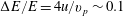 $\unicode[STIX]{x0394}E/E=4u/v_{p}\sim 0.1$
, i.e.
$\unicode[STIX]{x0394}E/E=4u/v_{p}\sim 0.1$
, i.e.
 $\unicode[STIX]{x0394}E\sim 300~\text{keV}$
which is smaller than the expected broadening due to stochastic acceleration.
$\unicode[STIX]{x0394}E\sim 300~\text{keV}$
which is smaller than the expected broadening due to stochastic acceleration.
In ascribing any measured energy shift and spectral broadening to the second-order Fermi mechanism, it must be noted that target charging, generation of static electric fields due to the escape of hot electrons and energy loss by collisions can all obscure the signal (Hicks et al. Reference Hicks, Li, Séguin, Ram, Frenje, Petrasso, Soures, Glebov, Meyerhofer and Roberts2000; Zylstra et al. Reference Zylstra, Frenje, Grabowski, Li, Collins, Fitzsimmons, Glenzer, Graziani, Hansen and Hu2015). Other experiments with the proposed set-up are evaluating these effects and indicate that the resulting distortions are in fact negligible (Chen et al. Reference Chen, Bott, Tzeferacos, Rigby, Bell, Bingham, Graziani, Katz, Koenig and Li2018).
We can interpret the spread due to turbulent motion of
 $\unicode[STIX]{x0394}E=300~\text{keV}$
, as a lower bound for detection. Therefore given plasma conditions as in table 1, and certainly for a 3 times stronger magnetic field, second-order Fermi acceleration of D–D fusion protons should be measurable at the NIF.
$\unicode[STIX]{x0394}E=300~\text{keV}$
, as a lower bound for detection. Therefore given plasma conditions as in table 1, and certainly for a 3 times stronger magnetic field, second-order Fermi acceleration of D–D fusion protons should be measurable at the NIF.
To summarise, we have presented a suitable experimental set-up for measuring stochastic acceleration of protons in a turbulent plasma. If realised, this would provide a platform where basic physical processes related to the classic Fermi theory of cosmic ray acceleration can be directly tested and validated against numerical simulations. We have demonstrated that the unique experimental capabilities available at NIF offer a potential route to explore collisionless magnetised transport, where unlike in previous studies (Chen et al.
Reference Chen, Bott, Tzeferacos, Rigby, Bell, Bingham, Graziani, Katz, Koenig and Li2018) the crossing time exceeds the scattering/isotropisation time. For the experimental conditions we consider, the transition occurs at turbulent field strengths of
 $B\lesssim 3$
MG, which are theoretically achievable using the experimental set-up of Tzeferacos et al. (Reference Tzeferacos, Rigby, Bott, Bell, Bingham, Casner, Cattaneo, Churazov, Emig and Fiuza2018). This regime may have practical implications for the acceleration of cosmic rays in the presence of sub-Larmor scale turbulent fields in astrophysical systems (e.g. Bell Reference Bell2004).
$B\lesssim 3$
MG, which are theoretically achievable using the experimental set-up of Tzeferacos et al. (Reference Tzeferacos, Rigby, Bott, Bell, Bingham, Casner, Cattaneo, Churazov, Emig and Fiuza2018). This regime may have practical implications for the acceleration of cosmic rays in the presence of sub-Larmor scale turbulent fields in astrophysical systems (e.g. Bell Reference Bell2004).
Acknowledgements
We would like to thank J. Foster for valuable input. The research leading to these results has received funding from AWE plc. and the Engineering and Physical Sciences Research Council (grant numbers EP/M022331/1, EP/N014472/1 and EP/P010059/1). S.S. acknowledges a Niels Bohr Professorship awarded by the Danish National Research Foundation. © British Crown Copyright 2018/AWE.


