1. INTRODUCTION
Precise relative attitude and position estimation between two spacecraft are crucial to many space missions today, such as spacecraft formation flying and rendezvous and docking. Presently, Vision-based Navigation (VISNAV) systems, consisting of an optical sensor combined with specific light sources (beacons), are usually used to determine the relative attitude and position within the range of a few hundred metres (Alonso et al., Reference Alonso, Crassidis and Junkins2000; Kim et al., Reference Kim, Crassidis, Cheng, Fosbury and Junkins2007; Xing et al., Reference Xing, Cao, Zhang, Guo and Wang2010; Tang et al., Reference Tang, Yan and Zhong2010). In order to determine the coupled attitude and position from the Line-Of-Sight (LOS) measurements, a Gaussian Least Squares Differential Correction (GLSDC) algorithm is usually used to provide a deterministic solution. To overcome the shortcoming of the iterative computation, Crassidis et al. (Reference Crassidis, Alonso and Junkins2000) presented an optimal attitude and position determination approach derived from a generalised predictive filter for nonlinear systems. However, these unitary vision-based estimation methods, which only utilise the static geometrical relations to determine the relative attitude and position are liable to be affected by the error factors, such as measurement errors, quantization errors, and extraction errors of the beacon locations, etc. Therefore, it is necessary to adopt the state estimation method to design a navigation filter. At present, two types of navigation filters include the absolute navigation filter (Wodffinden and Geller, Reference Wodffinden and Geller2007; Schmidt et al., Reference Schmidt, Geller and Chavez2010; Hablani, Reference Hablani2009) and the relative navigation filter (Alonso et al., Reference Alonso, Crassidis and Junkins2000; Kim et al., Reference Kim, Crassidis, Cheng, Fosbury and Junkins2007; Xing et al., Reference Xing, Cao, Zhang, Guo and Wang2010; Junkins et al., Reference Junkins, Hughes, Wazni and Pariyapong1999; Hablani et al., Reference Hablani, Tapper and Dana-Bashian2002). The absolute navigation system formulates the dynamics models of the two spacecraft in the inertial frame and acquires the relative motion parameters by computing the differences between two spacecraft. The relative navigation system estimates the relative position and velocity based on the relative equations of motion established in a rotating Local Vertical Local Horizontal (LVLH) frame. For close-range relative motion, the relative navigation system is usually adopted due to its sufficient accuracy and better computational efficiency.
The VISNAV system consists of an optical sensor combined with specific light sources (beacons) to achieve a selective vision. In general, the known beacon locations are defined in the master's body frame, whereas the relative position vector between the master and slave spacecraft is expressed in its LVLH frame. In Alonso et al. (Reference Alonso, Crassidis and Junkins2000), Kim et al. (Reference Kim, Crassidis, Cheng, Fosbury and Junkins2007) and Xing et al. (Reference Xing, Cao, Zhang, Guo and Wang2010), a simplified assumption that the master body frame coincides with its LVLH frame is made to construct the LOS observations for convenience. Unfortunately, this assumption is not valid under all situations, or in some rigorous senses, it is only a special case. One approach to solve this problem is to formulate the relative equations of motion in the master body frame (Tang et al., Reference Tang, Yan and Zhong2010), and thus the beacon location vectors and relative position vector are described in the same coordinates. The main disadvantages of this approach are that the angular velocity of the master body frame generally varies rapidly and its measured value is contaminated by the gyro measurement error. They may cause large computation errors in the relative equations of motion. Another approach is to additionally estimate the attitudes of both spacecraft relative to the LVLH frame (Zhang et al., Reference Zhang, Yang, Zhang, Cai and Qian2014), and the assumption that both the master's body and LVLH frames are the same can be removed.
The Extended Kalman Filter (EKF) is the most widely used for nonlinear filtering problems so far. The EKF operates by approximating the state distribution and relevant noise densities as Gaussian random variables (GRVs) and then propagating them through a first-order linearization of the nonlinear system (Wan and van der Merwe, Reference Wan and van der Merwe2001). Unfortunately, this can result in large errors in the true posterior means and covariances of the transformed GRVs, which may lead to suboptimal performance and sometimes divergence of the filter. To overcome this problem, the Unscented Kalman Filter (UKF) (Julier and Uhlmann, Reference Julier and Uhlmann1997; Julier et al., Reference Julier, Uhlmann and Durrant-Whyte2000) uses a deterministic sampling approach to approximate the state distribution as a GRV, which can capture the posterior mean and covariance accurately to at least second order for any nonlinearity. The UKF has proven to be far superior to the EKF, especially when accurate initial condition states are not well known. In addition, the UKF avoids the derivation of Jacobian matrices and has the same computational complexity as the EKF. The motivation of this paper is to derive a novel relative spacecraft attitude and position estimation approach based on an Unscented Kalman Filter. A quaternion-based method is used to describe the relative attitude kinematics. In order to maintain the quaternion normalization constraint in the filter, an unconstrained three-component vector of generalized Rodrigues parameters (GRPs) is used to represent quaternion error vectors and a multiplicative quaternion-error method is employed. This method was first proposed by Crassidis and used in the Unscented Quaternion Estimator (USQUE) (Crassidis and Markley, Reference Crassidis and Markley2003) and Inertial Navigation System/Global Positioning System (INS/GPS) integrated navigation systems (Crassidis, Reference Crassidis2005). To obtain the propagated sigma-point GRPs, the propagated sigma-point error quaternions should be first computed by multiplying the propagated sigma-point quaternions with a reference quaternion. Recently, Chang et al. (Reference Chang, Hu and Chang2014) pointed out that the better choice for the reference quaternion was not the sigma-point quaternion at the centre but the mean of the propagated sigma-point quaternions. It is reported that this can further improve the filtering performance when the nonlinearities of the dynamics model are severe or a good a priori estimate of the state is unavailable. An averaging-quaternion algorithm (Cheng et al., Reference Cheng, Markley, Crassidis and Oshman2007) is used to average a set of weighted sigma-point quaternions, which can maintain the unit-norm property of the quaternion. Thus, we adopt this scheme and give a modified version of the UKF. The performances of the EKF and two versions of the UKF with respect to initial condition errors are compared.
The organisation of this paper proceeds as follows. The Unscented Kalman Filter is briefly reviewed in Section 2. In Section 3, various reference frames used in this paper are summarised and a review of the relative equations of motion for eccentric orbits is provided. The relative quaternions that map the master's LVLH frame to the slave and master body frames are defined, and the corresponding relative quaternion kinematics equations are given. In Section 4, the gyro measurement model is reviewed and a stringent VISNAV measurement model for the LOS observations is shown. In Section 5, a brief review of the implementation equations for the EKF is shown, and a novel relative spacecraft attitude and position estimation approach based on UKF is derived. A modified UKF is also proposed based on the averaging-quaternion algorithm. In Section 6, simulation results are presented to compare the performances of the EKF and the UKF with respect to initial condition errors. Concluding remarks are given in Section 7.
2. UNSCENTED KALMAN FILTER
In this section, the UKF is reviewed. Consider the following discrete-time nonlinear dynamical system with additive process and measurement noises:
 $${\bi x}_k = {\bi f}({\bi x}_{k - 1}, k) + {\bi w}_{k - 1} $$
 $${\bi \tilde y}_k = {\bi h}\left( {x_k, k} \right) + {\bi v}_k $$
where xk∈ℝn is the state vector at time k;  ${\bi \tilde y}_k \in {\opf R}^m $ is the measurement vector at time k; f (·) and h (·) are known nonlinear functions; wk−1 and vk are independent Gaussian white process noise and measurement noise with covariances Qk−1 and Rk, respectively.
In the UKF, the Unscented Transformation (UT) is employed to calculate the statistics of a random variable which undergoes a nonlinear transformation. Compared with the EKF, the UKF has better convergence characteristics and greater accuracy for nonlinear systems. Furthermore, the UKF avoids the derivation of Jacobian matrices and has the same computational complexity as the EKF.
The entire algorithm is shown as follows (Wan and van der Merwe, Reference Wan and van der Merwe2001):
(a) Initialisation:
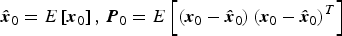
(3) $${\bi \hat x}_0 = E\left[ {{\bi x}_0} \right],{\kern 1pt} {\kern 1pt} {\bi P}_0 = E\left[ {\left( {{\bi x}_0 - {\bi \hat x}_0} \right)\left( {{\bi x}_0 - {\bi \hat x}_0} \right)^T} \right]$$
(b) Time update equations:
1) Evaluate the sigma points:
(4)where$${\bi X}_{k - 1} = \left[ {{\bi \hat x}_{k - 1} \;{\bi \hat x}_{k - 1} + \gamma \sqrt {{\bi P}_{k - 1}} \;{\bi \hat x}_{k - 1} - \gamma \sqrt {{\bi P}_{k - 1}} \;} \right]^T, \;{\kern 1pt} k = 1, \ldots, \infty $$$\gamma = \sqrt {n + \lambda} $, n is the dimension of the state, and λ=α 2(n+κ)−n is a composite scaling parameter. The constant α determines the spread of the sigma points and is usually chosen as a small positive value (e.g., 1×10⁻⁴⩽α⩽1). The constant κ is a secondary scaling parameter, which is usually chosen as κ=3−n.2) Evaluate the propagated sigma points (i=0, 1, … 2n)
(5)$${\bi X}_{k \vert k - 1}^* (i) = {\bi f}\left( {{\bi X}_{k - 1} (i)} \right)$$3) Estimate the predicted state and covariance matrix
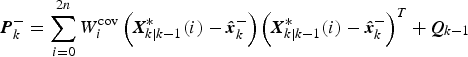
(6)$${\bi \hat x}_k^ - = \sum\limits_{i = 0}^{2n} {W_i^{{\rm mean}} {\bi X}_{k \vert k - 1}^* (i)} $$(7)The weights, W imean and W icov, are computed using$${\bi P}_k^ - = \sum\limits_{i = 0}^{2n} {W_i^{{\mathop{\rm cov}}} \left( {{\bi X}_{k \vert k - 1}^* (i) - {\bi \hat x}_k^ -} \right)\left( {{\bi X}_{k \vert k - 1}^* (i) - {\bi \hat x}_k^ -} \right)^T} + {\bi Q}_{k - 1} $$(8)where β is a nonnegative weighting coefficient for incorporating prior knowledge of the distribution (a good starting guess is β=2).$$\eqalign{W_0^{{\rm mean}} = & {\lambda / {(n + \lambda )}} \cr W_0^{{\mathop{\rm cov}}} = & W_0^{{\rm mean}} + (1 - \alpha ^2 + \beta ) \cr W_i^{{\mathop{\rm cov}}} = & W_i^{{\rm mean}} = {1 / {\left[ {2(n + \lambda )} \right]}}{\kern 1pt}, {\kern 1pt} \;i = 1, \ldots, {\kern 1pt} 2n} $$4) Redraw a complete new set of sigma points
(9)This alternative approach introduces fewer sigma points being used than the augmenting sigma point method (Wan and van der Merwe, Reference Wan and van der Merwe2001).$${\bi X}_{k \vert k - 1} = \left[ {{\bi \hat x}_k^ - \quad {\bi \hat x}_k^ - + \gamma \sqrt {{\bi P}_k^ -} \quad {\bi \hat x}_k^ - - \gamma \sqrt {{\bi P}_k^ -}} \right]^T $$5) Estimate the predicted measurement (i=0, 1, … 2n)
(10)$${\bf {\cal Y}}_{\left. k \right \vert k - 1} (i) = {\bi h}\left( {{\bi X}_{k \vert k - 1} (i)} \right)$$(11)$${\bi \hat y}_k^ - = \sum\limits_{i = 0}^{2n} {W_i^{{\rm mean}} {\bf {\cal Y}}_{\left. k \right \vert k - 1} (i)} $$
(c) Measurement update equations:
1) Estimate innovation covariance matrix and cross-covariance matrix
(12)$${\bi P}_{{\bf y}_k {\bf y}_k} = \sum\limits_{i = 0}^{2n} {W_i^{{\mathop{\rm cov}}} \left( {{\bf {\cal Y}}_{\left. k \right \vert k - 1} (i) - {\bi \hat y}_k^ -} \right)\left( {{\bf {\cal Y}}_{\left. k \right \vert k - 1} (i) - {\bi \hat y}_k^ -} \right)^T} + {\bi R}_k$$(13)$${\bi P}_{{\rm x}_k {\rm y}_k} = \sum\limits_{i = 0}^{2n} {W_i^{{\mathop{\rm cov}}} \left( {{\bi X}_{\left. k \right \vert k - 1} (i) - {\bi \hat x}_k^ -} \right)\left( {{\bf {\cal Y}}_{\left. k \right \vert k - 1} (i) - {\bi \hat y}_k^ -} \right)^T} $$2) Estimate the Kalman gain, updated state and covariance
(14)$${\bi K}_k = {\bi P}_{ {\rm x}_k {\rm y}_k} {\bi P}_{ {\rm y}_k {\rm y}_k} ^{ - 1}$$(15)$${\bi \hat x}_k^ + = {\bi \hat x}_k^ - + {\bi K}_k \left( {{\bi \tilde y}_k - {\bi \hat y}_k^ -} \right)$$(16)$${\bi P}_k^ + = {\bi P}_k^ - - {\bi K}_k {\bi P}_{{\rm y}_k {\rm y}_k} {\bi K}_k^T$$


For higher-dimensional systems, caution should be exercised when κ is negative since a possibility exists that the predicted covariance can become non-positive and semi-definite. A modified form of the prediction algorithm can be employed to overcome this problem (Julier and Uhlmann, Reference Julier and Uhlmann1997).
3. RELATIVE ORBITAL MOTION AND QUATERNION KINEMATICS
In this section, an overview of the general relative equations of motion for eccentric orbits and the quaternion kinematics is shown. Two relative quaternions that map the master's LVLH frame to the master body frame and to the slave body frame are defined. The corresponding relative quaternion kinematics equations are derived.
3.1. Reference Frames
(1) Earth-Centred-Inertial (ECI) frame (I frame): The frame has its origin at the centre of the Earth and is non-rotating with respect to the stars (except for precession of equinoxes). The z axis points in the direction of the North pole, the x axis points in the direction of the Earth's prime meridian, and the y axis completes the right-handed system.
(2) Local-Vertical-Local-Horizontal (LVLH) frame (H frame): The LVLH frame is centred at the master spacecraft body, the x axis is directed from the spacecraft radially outward and often labelled as the R-bar, z axis is normal to the master's orbital plane, and y axis is defined as the cross-product of the other two axes.
(3) Body Frame: This frame is fixed onto the spacecraft body and rotates with it. Body frames fixed to the two spacecraft are designated as master (m frame) and slave (s frame), respectively.
3.2. Relative Orbital Motion Equations
In this section, the relative equations of motion using Cartesian coordinates in the rotating LVLH frame are summarised. The relative orbit position vector ρ is expressed in the master's LVLH frame components as ρ=[x, y, z]T. If the relative orbit coordinates are small compared to the master orbit radius, the general relative equations of motion for eccentric orbits are given by (Kim et al., Reference Kim, Crassidis, Cheng, Fosbury and Junkins2007)
 $$\eqalign{\ddot x - x\dot \theta ^2 \left( {1 + 2\displaystyle{{r_m} \over p}} \right) - & 2\dot \theta \left( {\dot y - y\displaystyle{{\dot r_m} \over {r_m}}} \right) = \varpi _x \cr \ddot y + 2\dot \theta \left( {\dot x - x\displaystyle{{\dot r_m} \over {r_m}}} \right) - & y\dot \theta ^2 \left( {1 - \displaystyle{{r_m} \over p}} \right) = \varpi _y \cr & \ddot z + z\dot \theta ^2 \displaystyle{{r_m} \over p} = \varpi _z} $$
where p, r m and  $\dot \theta $ are the semilatus rectum, orbit radius and true anomaly rate of the master spacecraft, respectively. The acceleration disturbance vector ϖ≡[ϖ xϖ yϖz]T is modelled as a zero-mean Gaussian white-noise process with
 $$E\left\{ {{\bi \varpi} (t){\bi \varpi} ^T (\tau )} \right\} = \sigma _\varpi ^2 \delta (t - \tau ){\bi I}_{3 \times 3} $$
The true anomaly acceleration and orbit-radius acceleration of the master spacecraft are given by
 $$\ddot \theta = - 2\displaystyle{{\dot r_m} \over {r_m}} \dot \theta \quad \ddot r_m = r_m \dot \theta ^2 \left( {1 - \displaystyle{{r_m} \over p}} \right)$$
Thus, a ten-dimensional nonlinear state-space model can be derived by using Equations (17) and (19). The state vector xp consists of relative position and velocity of the slave, radius and radial rate as well as the true anomaly and rate of the master, given by
 $$\eqalign{{\bi x}_p & = \left[ {\matrix{ x & y & z & {\dot x} & {\dot y} & {\dot z} & {r_m} & {\dot r_m} & \theta & {\dot \theta} \cr}} \right]^T \cr & \equiv \left[ {\matrix{ {x_{\,p_1}} & {x_{\,p_2}} & {x_{\,p_3}} & {x_{\,p_4}} & {x_{\,p_5}} & {x_{\,p_6}} & {x_{\,p_7}} & {x_{\,p_8}} & {x_{\,p_9}} & {x_{\,p_{10}}} \cr}} \right]^T} $$
Using Equations (17) and (19), the ten-dimensional nonlinear differential equations are given by
 $${\bi \dot x}_p = {\bi f}\left( {{\bi x}_p} \right) \equiv \left[ {\matrix{ {x_{\,p_4}} \cr {x_{\,p_5}} \cr {x_{\,p_6}} \cr {x_{\,p_1} x_{\,p_{10}} ^2 \left( {1 + 2x_{\,p_7} /p} \right) + 2x_{\,p_{10}} \left( {x_{\,p_5} - x_{\,p_2} x_{\,p_8} /x_{\,p_7}} \right)} \cr { - 2x_{\,p_{10}} \left( {x_{\,p_4} - x_{\,p_1} x_{\,p_8} /x_{\,p_7}} \right) + x_{\,p_2} x_{\,p_{10}} ^2 \left( {1 - x_{\,p_7} /p} \right)} \cr { - x_{\,p_7} x_{\,p_{10}} ^2 x_{\,p_3} /p} \cr {x_{\,p_8}} \cr {x_{\,p_7} x_{\,p_{10}} ^2 \left( {1 - x_{\,p_7} /p} \right)} \cr {x_{\,p_{10}}} \cr { - 2x_{\,p_8} x_{\,p_{10}} /x_{\,p_7}} \cr}} \right]$$
3.3. Relative Quaternion Kinematics
In this section a brief review of the relative quaternion kinematics between two rotated coordinate systems is shown. The quaternion is defined by q≡ [ϱT q4]T, with ϱ≡[q 1q 2q 3]T=e sin (ϕ/2) and q 4=cos(ϕ/2), where e is the unit Euler axis and ϕ is the rotation angle (Shuster, Reference Shuster1993). The quaternion q obeys the unit normalisation constraint given by ||q||=1. The attitude matrix is related to the quaternion by
 $${\bi A}({\bi q}) = \left( {q_4^2 - \| {\bi \varrho} \|^2} \right){\bi I}_{3 \times 3} + 2{\bi \varrho \varrho} ^{\rm T} - 2q_4 [{\bi \varrho} \times ] = \Xi ^T ({\bi q}){\rm \Psi} ({\bi q})$$
With
 $$\Xi ({\bi q}) \equiv \left[ {\matrix{ {q_4 {\bi I}_{3 \times 3} + \left[ {{\bi \varrho} \times} \right]} \cr { - {\bi \varrho} ^{\rm T}} \cr}} \right]\quad {\rm \Psi} ({\bi q}) \equiv \left[ {\matrix{ {q_4 {\bi I}_{3 \times 3} - \left[ {{\bi \varrho} \times} \right]} \cr { - {\bi \varrho} ^{\rm T}} \cr}} \right]$$
where I3×3 is a 3×3 identity matrix and [ϱ×] is a cross product matrix defined by
 $$\left[ {{\bi \varrho} \times} \right] \equiv \left[ {\matrix{ 0 & { - q_3} & {q_2} \cr {q_3} & 0 & { - q_1} \cr { - q_2} & {q_1} & 0 \cr}} \right]$$
Successive rotations can be accomplished by using quaternion multiplication. In this paper, quaternion multiplication is defined using the convention of Lefferts et al. (Reference Lefferts, Markley and Shuster1982) in which the quaternion multiplication expression appears in the same order as the corresponding attitude matrix multiplication: A(q′)A(q)=A(q′⊗q). The composition of the quaternions is bilinear, with
 $${\bi q'} \otimes {\bi q} = \left[ {\matrix{ {{\rm \Psi} ({\bi q'})} & {{\bi q'}} \cr}} \right]{\bi q =} \left[ {\matrix{ {\Xi ({\bi q})} & {\bi q} \cr}} \right]{\bi q'}$$
The quaternion kinematics equation is given by
 $${\bi \dot q =} \displaystyle{1 \over 2}\Xi ({\bi q}){\bi \omega} = \displaystyle{1 \over 2}{\rm \Omega} ({\bi \omega} ){\bi q}$$
where ω is the three-component angular rate vector and
 $${\rm \Omega} ({\bi \omega} ) \equiv \left[ {\matrix{ { - \left[ {{\bi \omega} \times} \right]} & {\bi \omega} \cr { - {\bi \omega} ^{\rm T}} & {\rm 0} \cr}} \right]$$
The relative quaternions qs/H and qm/H, which map the master's LVLH frame (H frame) to the slave body frame (s frame) and to the master body frame (m frame), are defined as
 $${\bi q}_{s/H} = {\bi q}_s \otimes {\bi q}_H^{ - 1}, \,{\bi q}_{m/H} = {\bi q}_m \otimes {\bi q}_H^{ - 1} $$
where qs, qm and q H are the inertial attitudes of the slave body frame, master body frame and master's LVLH frame, respectively. The relative quaternion kinematics equations are given by (Mayo, Reference Mayo1979)
 $${\bi \dot q}_{s/H} = \displaystyle{1 \over 2}\Xi ({\bi q}_{s/H} ){\bi \omega} _{s/H}^s, \;{\bi \dot q}_{m/H} = \displaystyle{1 \over 2}\Xi ({\bi q}_{m/H} ){\bi \omega} _{m/H}^m $$
where ωs/Hs is the angular velocity of the s frame relative to the H frame expressed in s coordinates, and ωm/Hm is the angular velocity of the m frame relative to the H frame expressed in m coordinates. They are defined as
 $${\bi \omega} _{s/H}^s \equiv {\bi \omega} _{s/I}^s - {\bi A}_H^s ({\bi q}_{s/H} ){\bi \omega} _{H/I}^H $$
 $${\bi \omega} _{m/H}^m \equiv {\bi \omega} _{m/I}^m - {\bi A}_H^m ({\bi q}_{m/H} ){\bi \omega} _{H/I}^H $$
where ωs/Is and ωm/Im are the inertial angular velocities of the slave and master spacecraft, respectively; AHs and AHm are the attitude matrices that convert vectors from the H frame to the s frame and to the m frame, respectively; and ωH/IH is the angular velocity of master's H frame expressed in H coordinates defined as
 $${\bi \omega} _{H/I}^H = \left[ {\matrix{ 0 & 0 & {\dot \theta} \cr}} \right]^T $$
A discrete-time propagation of Equation (29) is given by (Mayo, Reference Mayo1979)
 $${\bi q}_{s/H_{k + 1}} = {\rm \bar \Omega} \left( {{\bi \omega} _{s/I}^s} \right){\rm \bar \Gamma} \left( {{\bi \omega} _{H/I}^H} \right){\bi q}_{s/H_k} $$
With
 $${\rm \bar \Omega} \left( {{\bi \omega} _{s/I}^s} \right) = \left[ {\matrix{ {\cos \left( {{\textstyle{1 \over 2}}\| {{\bi \omega} _{s/I}^s} \| {\rm \Delta} t} \right){\bi I}_{3 \times 3} - \left[ {{\bi \psi} _k \times} \right]} & {{\bi \psi} _k} \cr { - {\bi \psi} _k^T} & {\cos \left( {{\textstyle{1 \over 2}}\| {{\bi \omega} _{s/I}^s} \| {\rm \Delta} t} \right)} \cr}} \right]$$
 $${\rm \bar \Gamma} \left( {{\bi \omega} _{H/I}^H} \right) = \left[ {\matrix{ {\cos \left( {{\textstyle{1 \over 2}}\| {{\bi \omega} _{H/I}^H} \| {\rm \Delta} t} \right){\bi I}_{3 \times 3} - \left[ {{\bi \zeta} _k \times} \right]} & { - {\bi \zeta} _k} \cr {{\bi \zeta} _k^T} & {\cos \left( {{\textstyle{1 \over 2}}\| {{\bi \omega} _{H/I}^H} \| {\rm \Delta} t} \right)} \cr}} \right]$$
where
 $$\eqalign{& {\bi \psi} _k \equiv {{\sin \left( {{\textstyle{1 \over 2}}\| {{\bi \omega} _{s/I}^s} \| {\rm \Delta} t} \right){\bi \omega} _{s/I}^s} / {\| {{\bi \omega} _{s/I}^s} \| }} \cr & {\bi \zeta} _k \equiv {{\sin \left( {{\textstyle{1 \over 2}}\| {{\bi \omega} _{H/I}^H} \| {\rm \Delta} t} \right){\bi \omega} _{H/I}^H} / {\| {{\bi \omega} _{H/I}^H} \| }}} $$
and Δt is the sampling interval.
Likewise, the discrete-time propagation of the relative quaternion qm/H is given by
 $${\bi q}_{m/H_{k + 1}} = {\rm \bar \Omega} \left( {{\bi \omega} _{m/I}^m} \right){\rm \bar \Gamma} \left( {{\bi \omega} _{H/I}^H} \right){\bi q}_{m/H_k} $$
where  ${\rm \bar \Omega} ( {{\bi \omega} _{m/I}^m} )$ can be obtained by substituting ωm/Im for ωs/Is in Equation (34).
The relative attitude quaternion that maps the master body frame to the slave body frame is obtained by
 $${\bi q}_{s/m} = {\bi q}_{s/H} \otimes {\bi q}_{m/H}^{ - 1} $$
4. SENSOR MODELS
In this section the VISNAV measurement model and gyro measurement model are reviewed. The corresponding attitude matrices for the relative quaternions mentioned above are used to construct the LOS observations, and the assumption that both the master body and LVLH frames are the same can be removed.
4.1. VISNAV Measurement Model
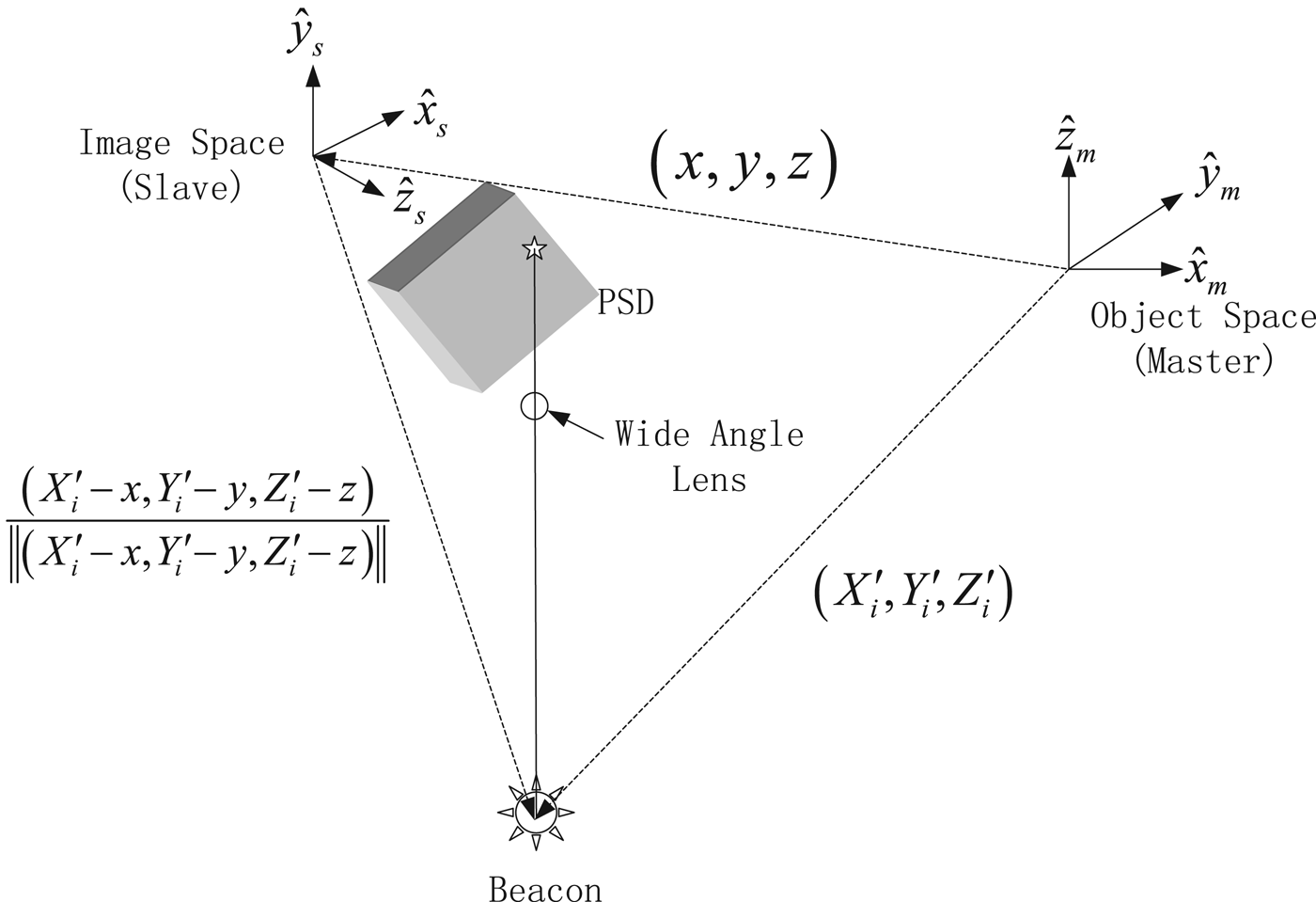
The VISNAV system consists of an optical sensor combined with specific light sources (beacons), which can be used for close range photogrammetry-type applications (Kim et al., Reference Kim, Crassidis, Cheng, Fosbury and Junkins2007). In general, the beacon locations are known within the master body frame and the sensor focal plane location is known within the slave body frame. Without loss of generality, the assumption that the master body frame coincides with its LVLH frame is not made here. An illustration of the VISNAV system is provided in Figure 1. The measurement model in unit vector form for the i th LOS is given by
 $${\bi \tilde b}_i = {\bi A}_H^s \left( {{\bi q}_{s/H}} \right){\bi r}_i + {\bi \upsilon} _i, \quad {\bi \upsilon} _i ^T {\bi A}_H^s {\bi r}_i = 0$$
with
 $${\bi r}_i \equiv \displaystyle{{{\bf {\cal X}}_i ^\prime - {\bi \rho}} \over {\| {{\bf {\cal X}}_i ^\prime - {\bi \rho}} \| }} = \displaystyle{1 \over {\sqrt {\left( {X'_i - x} \right)^2 + \left( {Y'_i - y} \right)^2 + \left( {Z'_i - z} \right)^2}}} \left[ {\matrix{ {\left( {X'_i - x} \right)} \cr {\left( {Y'_i - y} \right)} \cr {\left( {Z'_i - z} \right)} \cr}} \right]$$
where  ${\bi \tilde b}_i $ denotes the measured unit vector for the i th beacon in the s frame, and (x, y, z) are the relative position coordinates modelled by Equation (17). ${\bf {\cal X}}'_i \equiv \left( {X'_i \;,Y'_i \;,\;Z'_i} \right)$ are the coordinates of the i th beacon with respect to the master body frame expressed in the H frame, given by
 $${\bf {\cal X}}_i ^\prime = \left[ {{\bi A}_H^m \left( {{\bi q}_{m/H}} \right)} \right]^T {\bf {\cal X}}_i $$
where  ${\bf {\cal X}}_i \equiv \left( {X_i, \;Y_i, \;Z_i} \right)$ are the known coordinates of the i th beacon with respect to the master body frame expressed in the m frame.

Figure 1. Vision-based navigation system.
The sensor measurement noise υi in Equation (39) is approximately Gaussian which satisfies
 $$E\left\{ {{\bi \upsilon} _i} \right\} = {\bf 0}$$
 $$E\left\{ {{\bi \upsilon} _i {\bi \upsilon} _i^T} \right\} = \sigma _i^2 \left[ {{\bi I}_{3 \times 3} - \left( {{\bi A}_H^s {\bi r}_i} \right)\left( {{\bi A}_H^s {\bi r}_i} \right)^T} \right]$$
and E{·} denotes expectation. Equation (43) is known as the QUEST measurement model, which is quite accurate for small field-of-view sensors. According to Shuster (Reference Shuster1990), the measurement covariance matrix in Equation (43) can be replaced by σ i2I3×3. Multiple vector measurements can be expressed as
 $${\bi y}_k = \left[ {\matrix{ {{\bi \tilde b}_1} \cr {{\bi \tilde b}_2} \cr \vdots \cr {{\bi \tilde b}_N} \cr}} \right]_k = \left[ {\matrix{ {{\bi A}_H^s \left( {{\bi q}_{s/H}} \right){\bi r}_1} \cr {{\bi A}_H^s \left( {{\bi q}_{s/H}} \right){\bi r}_2} \cr \vdots \cr {{\bi A}_H^s \left( {{\bi q}_{s/H}} \right){\bi r}_N} \cr}} \right]_k + \left[ {\matrix{ {{\bi \upsilon} _1} \cr {{\bi \upsilon} _2} \cr \vdots \cr {{\bi \upsilon} _N} \cr}} \right]_k $$
where N is the total number of observations. The corresponding measurement noise covariance matrix is given by
 $${\bi R}_k = {\rm blkdiag}\left[ {\sigma _1^2 {\bi I}_{3 \times 3} \quad\sigma _2^2 {\bi I}_{3 \times 3} \; \cdots \;\sigma _N^2 {\bi I}_{3 \times 3}} \right]$$
where “blkdiag” denotes a block diagonal matrix of appropriate dimension.
4.2. Gyro Measurement Model
The common gyro measurement model is given by (Farrenkopf, Reference Farrenkopf1978)
 $$\eqalign{{\bi \tilde \omega} = & {\bi \omega} + {\bi \beta} + {\bi \eta} _\upsilon \cr & {\bi \dot \beta = \eta} _u} $$
where ω is the true inertial angular rate,  ${\bi \tilde \omega} $ is the measured inertial angular rate, β is the drift, and η υ and η u are independent zero-mean Gaussian white-noise processes with
 $$\eqalign{& E\left\{ {{\bi \eta} _\upsilon (t){\bi \eta} _\upsilon ^T (\tau )} \right\} = \sigma _\upsilon ^2 \delta (t - \tau ){\bi I}_{3 \times 3} \cr & E\left\{ {{\bi \eta} _u (t){\bi \eta} _u^T (\tau )} \right\} = \sigma _u^2 \delta (t - \tau ){\bi I}_{3 \times 3}} $$
where δ (t−τ) is the Dirac delta function. The discrete-time gyro measurements can be generated using the following recursive equations (Crassidis, Reference Crassidis2005):
 $${\bi \tilde \omega} _{k + 1} = {\bi \omega} _{k + 1} + \displaystyle{1 \over 2}\left( {{\bi \beta} _{k + 1} + {\bi \beta} _k} \right) + \left( {\displaystyle{{\sigma _\upsilon ^2} \over {{\rm \Delta} t}} + \displaystyle{1 \over {12}}\sigma _u^2 {\rm \Delta} t} \right)^{1/2} {\bi N}_{\upsilon k} $$
 $${\bi \beta} _{k + 1} = {\bi \beta} _k + \sigma _u {\rm \Delta} t^{1/2} {\bi N}_{uk} $$
where the subscript k denotes the k th time-step, Δt is the gyro sampling interval, and Nυk and Nuk are zero-mean Gaussian white-noise processes with covariance each given by the identity matrix.
5. RELATIVE ATTITUDE AND POSITION ESTIMATION
In this section, the EKF and UKF implementation equations for relative spacecraft attitude and position estimation are shown.
5.1. Relative Attitude and Position Estimation Using Extended Kalman Filter
As mentioned in the previous section, the estimation equations are given by
 $${\bi \dot {\hat q}}_{s/H} = \displaystyle{1 \over 2}\Xi \left( {{\bi \hat q}_{s/H}} \right){\bi \hat \omega} _{s/H}^s $$
 $${\bi \hat \omega} _{s/H}^s = {\bi \hat \omega} _{s/I}^s - {\bi A}_H^s \left( {{\bi \hat q}_{s/H}} \right){\bi \hat \omega} _{H/I}^H $$
 $${\bi \dot {\hat q}}_{m/H} = \displaystyle{1 \over 2}\Xi \left( {{\bi \hat q}_{m/H}} \right){\bi \hat \omega} _{m/H}^m $$
 $${\bi \hat \omega} _{m/H}^m = {\bi \hat \omega} _{m/I}^m - {\bi A}_H^m \left( {{\bi \hat q}_{m/H}} \right){\bi \hat \omega} _{H/I}^H $$
 $${\bi \hat \omega} _{s/I}^s = {\bi \tilde \omega} _{s/I}^s - {\bi \hat \beta} _s $$
 $${\bi \hat \omega} _{m/I}^m = {\bi \tilde \omega} _{m/I}^m - {\bi \hat \beta} _m $$
 $${\bi \dot {\hat x}}_p = f\left( {{\bi \hat x}_p} \right)$$
 $${\bi \hat \omega} _{H/I}^H = \left[ {\matrix{ 0 & 0 & {\hat {\dot \theta}} \cr}} \right]^T $$
 $${\bi \dot {\hat \beta}} _s = {\bf 0}$$
 $${\bi \dot{ \hat \beta}} _m = {\bf 0}$$
The state and error-state vectors are defined as
 $$\eqalign{{\bi x} \equiv & \left[ {\matrix{ {{\bi q}_{s/H}^T} & {{\bi q}_{m/H}^T} & {{\bi \beta} _s^T} & {{\bi \beta} _m^T} & {{\bi x}_p^T} \cr}} \right]^T \cr = & \left[ {\matrix{ {{\bi q}_{s/H}^T} & {{\bi q}_{m/H}^T} & {{\bi \beta} _s^T} & {{\bi \beta} _m^T} & {{\bi \rho} ^T} & {{\bi \dot \rho} ^T} & {r_m} & {\dot r_m} & \theta & {\dot \theta} \cr}} \right]^T} $$
 $$\Delta {\bi x} \equiv \left[ {\matrix{ {\delta {\bi \alpha} _{s/H}^T} & {\delta {\bi \alpha} _{m/H}^T} & {{\rm \Delta} {\bi \beta} _s^T} & {{\rm \Delta} {\bi \beta} _m^T} & {{\rm \Delta} {\bi \rho} ^T} & {{\rm \Delta} {\bi \dot \rho} ^T} & {{\rm \Delta} r_m} & {{\rm \Delta} \dot r_m} & {{\rm \Delta} \theta} & {{\rm \Delta} \dot \theta} \cr}} \right]^T $$
where δα is the vector of small attitude (roll, pitch and yaw) errors, and the other error-state terms Δ• are defined as  ${\rm \Delta} \bullet \equiv \bullet - \hat \bullet $.
According to the derivations in Zhang et al. (Reference Zhang, Yang, Zhang, Cai and Qian2014), the error-state dynamics equations used in the EKF propagation are given by
 $${\rm \Delta} {\bi \dot x} = {\bi F}{\rm \Delta} {\bi x} + {\bi Gw}$$
where the matrices F, G, process noise vector w and spectral density matrix Q are given by
 $${\bi F} \equiv \left[ {\matrix{ { - \left[ {{\bi \hat \omega} _{s/I}^s \times} \right]} & {{\bf 0}_{3 \times 3}} & { - {\bi I}_{3 \times 3}} & {{\bf 0}_{3 \times 3}} & {{\bf 0}_{3 \times 9}}\quad { - {\bi A}_H^s \left( {{\bi \hat q}_{s/H}} \right){\bi n}} \cr {{\bf 0}_{3 \times 3}} & { - \left[ {{\bi \hat \omega} _{m/I}^m \times} \right]} & {{\bf 0}_{3 \times 3}} & { - {\bi I}_{3 \times 3}} & {{\bf 0}_{3 \times 9}} \quad{ - {\bi A}_H^m \left( {{\bi \hat q}_{m/H}} \right){\bi n}} \cr {{\bf 0}_{3 \times 3}} & {{\bf 0}_{3 \times 3}} & {{\bf 0}_{3 \times 3}} & {{\bf 0}_{3 \times 3}} & {{\bf 0}_{3 \times 10}} & \cr {{\bf 0}_{3 \times 3}} & {{\bf 0}_{3 \times 3}} & {{\bf 0}_{3 \times 3}} & {{\bf 0}_{3 \times 3}} & {{\bf 0}_{3 \times 10}} & {} \cr {{\bf 0}_{10 \times 3}} & {{\bf 0}_{10 \times 3}} & {{\bf 0}_{10 \times 3}} & {{\bf 0}_{10 \times 3}} & {\left. {\displaystyle{{\partial f\left( {{\bi x}_p} \right)} \over {\partial {\bi x}_p}}} \right \vert _{{\bi \hat x}_p}} & \cr}} \right],\quad {\bi n} = \left[ {\matrix{ 0 & 0 & 1 \cr}} \right]^T $$
 $${\bi G} \equiv \left[ {\matrix{ { - {\bi I}_{3 \times 3}} & {{\bf 0}_{3 \times 3}} & {{\bf 0}_{3 \times 3}} & {{\bf 0}_{3 \times 3}} & {{\bf 0}_{3 \times 3}} \cr {{\bf 0}_{3 \times 3}} & { - {\bi I}_{3 \times 3}} & {{\bf 0}_{3 \times 3}} & {{\bf 0}_{3 \times 3}} & {{\bf 0}_{3 \times 3}} \cr {{\bf 0}_{3 \times 3}} & {{\bf 0}_{3 \times 3}} & {{\bi I}_{3 \times 3}} & {{\bf 0}_{3 \times 3}} & {{\bf 0}_{3 \times 3}} \cr {{\bf 0}_{3 \times 3}} & {{\bf 0}_{3 \times 3}} & {{\bf 0}_{3 \times 3}} & {{\bi I}_{3 \times 3}} & {{\bf 0}_{3 \times 3}} \cr {{\bf 0}_{3 \times 3}} & {{\bf 0}_{3 \times 3}} & {{\bf 0}_{3 \times 3}} & {{\bf 0}_{3 \times 3}} & {{\bf 0}_{3 \times 3}} \cr {{\bf 0}_{3 \times 3}} & {{\bf 0}_{3 \times 3}} & {{\bf 0}_{3 \times 3}} & {{\bf 0}_{3 \times 3}} & {{\bi I}_{3 \times 3}} \cr {{\bf 0}_{2 \times 3}} & {{\bf 0}_{2 \times 3}} & {{\bf 0}_{2 \times 3}} & {{\bf 0}_{2 \times 3}} & {{\bf 0}_{2 \times 3}} \cr {{\bf 0}_{2 \times 3}} & {{\bf 0}_{2 \times 3}} & {{\bf 0}_{2 \times 3}} & {{\bf 0}_{2 \times 3}} & {{\bf 0}_{2 \times 3}} \cr}} \right]$$
 $${\bi w} \equiv \left[ {\matrix{ {{\bi \eta} _{s\upsilon} ^T} & {{\bi \eta} _{m\upsilon} ^T} & {{\bi \eta} _{su}^T} & {{\bi \eta} _{mu}^T} & {{\bi \varpi} ^T} \cr}} \right]^T $$
 $${\bi Q} = {\rm blkdiag}\left[ {\matrix{ {\sigma _{s\upsilon} ^2 {\bi I}_{3 \times 3}} & {\sigma _{m\upsilon} ^2 {\bi I}_{3 \times 3}} & {\sigma _{su}^2 {\bi I}_{3 \times 3}} & {\sigma _{mu}^2 {\bi I}_{3 \times 3}} & {\sigma _\varpi ^2 {\bi I}_{3 \times 3}} \cr}} \right]$$
The complete EKF implementation equations are given in Zhang et al. (Reference Zhang, Yang, Zhang, Cai and Qian2014) and are not shown here for brevity.
5.2. Relative Attitude and Position Estimation Using Unscented Kalman Filter
5.2.1. UKF1
In the UKF design, since the predicted quaternion mean is computed by using an averaged sum of quaternions, the resulting quaternion cannot be guaranteed to have the unit-norm constraint. In order to overcome this problem, an unconstrained three-component vector of Generalised Rodrigues Parameters (GRPs) is used to propagate and update a nominal quaternion, which is defined by (Crassidis and Markley, Reference Crassidis and Markley2003)
 $$\delta {\bi p} \equiv f\displaystyle{{\delta {\bi \varrho}} \over {a + \delta q_4}} $$
where a is a parameter from 0 to 1, and f is a scale factor. Notice that when a=0 and f=1 then Equation (67) gives the Gibbs vector, and when a=1 and f=1 then Equation (67) gives the standard vector of Modified Rodrigues Parameters (MRPs). We will choose f=2(a+1) so that ||δp|| is equal to the rotational error-angle for small errors.
We start by defining the following state vector:
 $${\bi X}_k (0) = {\bi \hat x}_k^ + \equiv \left[ {\matrix{ {\delta {\bi \hat p}_{s/H_k} ^ +} \cr {\delta {\bi \hat p}_{m/H_k} ^ +} \cr {{\bi \hat \beta} _{s_k} ^ +} \cr {{\bi \hat \beta} _{m_k} ^ +} \cr {{\bi \hat x}_{\,p_k} ^ +} \cr}} \right],\;{\bi X}_k (i) \equiv \left[ {\matrix{ {{\bi X}_k^{\delta {\bi p}_{s/H}} (i)} \cr {{\bi X}_k^{\delta {\bi p}_{m/H}} (i)} \cr {{\bi X}_k^{{\bi \beta} _s} (i)} \cr {{\bi X}_k^{{\bi \beta} _m} (i)} \cr {{\bi X}_k^{{\bi x}_p} (i)} \cr}} \right]\;,\;{\bi X}_k^{{\bi x}_p} (i) \equiv \left[ {\matrix{ {{\bi X}_k^{\bi \rho} (i)} \cr {{\bi X}_k^{{\bi \dot \rho}} (i)} \cr {{\bi X}_k^{r_m} (i)} \cr {{\bi X}_k^{\dot r_m} (i)} \cr \matrix{{\bi X}_k^\theta (i) \cr {\bi X}_k^{\dot \theta} (i) } \cr}} \right],\quad i = 1,2,...44$$
where  ${\bi X}_k^{\delta {\bi p}_{s/H}} $ and ${\bi X}_k^{\delta {\bi p}_{m/H}} $ are from the attitude-error parts of relative quaternions qs/H and qm/H, respectively; ${\bi X}_k^{{\bi \beta} _s} $ and ${\bi X}_k^{{\bi \beta} _m} $ are from the gyro drift parts for the slave and master spacecraft, respectively; ${\bi X}_k^{{\bi x}_p} $ is from the part of ten-dimensional state vector xp. In order to describe ${\bi X}_k^{\delta {\bi p}_{s/H}} $ and ${\bi X}_k^{\delta {\bi p}_{m/H}} $, we need to define a new quaternion generated by multiplying an error quaternion by the current estimate. Take ${\bi X}_k^{\delta {\bi p}_{s/H}} $ for instance, the following quaternions are firstly computed:
 $${\bi \hat q}_{s/H_k} ^ + (0) = {\bi \hat q}_{s/H_k} ^ + $$
 $${\bi \hat q}_{s/H_k} ^ + (i) = \delta {\bi \hat q}_{s/H_k} ^ + (i) \otimes {\bi \hat q}_{s/H_k} ^ +, \quad i = 1,2, \ldots, 44$$
where  $\delta {\bi \hat q}_{s/H_k} ^ + (i) \equiv \left[ {\delta {\bi \varrho} _{s/H_k} ^{ + T} (i)\;\delta q_{4,s/H_k} ^ + (i)} \right]^T $ is represented by
 $$\delta q_{4,s/H_k} ^ + (i) = \displaystyle{{ - a\| {{\bi X}_k^{\delta {\bi p}_{s/H}} \left( i \right)} \| ^2 + f\sqrt {\,f^2 + \left( {1 - a^2} \right)\| {{\bi X}_k^{\delta {\bi p}_{s/H}} (i)} \| ^2}} \over {\,f^2 + \| {{\bi X}_k^{\delta {\bi p}_{s/H}} (i)} \| ^2}}, \quad i = 1,2, \ldots, 44$$
 $$\delta {\bi \varrho} _{s/H_k} ^ + (i) = f^{ - 1} \left[ {a + \delta q_{4,s/H_k} ^ + (i)} \right]{\bi X}_k^{\delta {\bi p}_{s/H}} (i),\quad i = 1,2,...,44$$
Next, the sigma-point quaternions in Equation (70) are propagated forward using Equation (33), with
 $${\bi \hat q}^ - _{s/H_{k + 1}} (i) = {\rm \bar \Omega} \left( {{\bi \hat \omega} _{s/I_k} ^{s +} (i)} \right){\rm \bar \Gamma} \left( {{\bi \hat \omega} _{H/I_k} ^{H +} (i)} \right){\bi \hat q}^{\bi +} _{s/H_k} (i),\quad i = 0,1, \ldots, 44$$
in which the estimated inertial angular velocities of the slave spacecraft are given by
 $${\bi \hat \omega} _{s/I_k} ^{s +} (i) = {\bi \tilde \omega} _{s/I_k} ^s - {\bi X}_k^{{\bi \beta} _s} (i),\quad i = 0,1,...,44$$
and the estimated angular velocities of the master's H frame are given by
 $${\bi \hat \omega} _{H/I_k} ^{H +} (i) = \left[ {\matrix{ 0 & 0 & {{\bi X}_k^{\dot \theta} (i)} \cr}} \right]^T, \quad i = 0,1,...,44$$
The propagated error quaternions are then computed using
 $$\delta {\bi \hat q}_{s/H_{k + 1}} ^ - (i) = {\bi \hat q}_{s/H_{k + 1}} ^ - (i) \otimes \left[ {{\bi \hat q}_{s/H_{k + 1}} ^ - (0)} \right]^{ - 1}, \quad i = 0,1, \ldots, 44$$
Notice that  $\delta {\bi \hat q}_{s/H_{k + 1}} ^ - (0)$ is the identity quaternion. Finally, the propagated sigma-point GRPs are computed using Equation (67) as
 $${\bi X}_{k + 1}^{\delta {\bi p}_{s/H}} (0) = {\bf 0}$$
 $${\bi X}_{k + 1}^{\delta {\bi p}_{s/H}} (i) = f\displaystyle{{\delta {\bi \varrho} _{s/H_{k + 1}} ^ - (i)} \over {a + \delta q_{4,s/H_{k + 1}} ^ - (i)}},\quad i = 1,2, \ldots, 44$$
with  $\left[ {\delta {\bi \varrho} _{s/H_{k + 1}} ^{ - T} (i)\;\delta q_{4,s/H_{k + 1}} ^ - (i)} \right]^T = \delta {\bi \hat q}_{s/H_{k + 1}} ^ - (i)$. Likewise, the sigma-point GRPs ${\bi X}_k^{\delta {\bi p}_{m/H}} $ can be propagated in the same manner.
In addition, notice that as the gyro drifts are expected to stay at their previous values (due to zero-mean process noises), we have
 $${\bi X}_{k + 1}^{{\bi \beta} _s} (i) = {\bi X}_k^{{\bi \beta} _s} (i),\;{\bi X}_{k + 1}^{{\bi \beta} _m} (i) = {\bi X}_k^{{\bi \beta} _m} (i),\quad \;i = 0,1, \ldots 44$$
All other sigma-point quantities formed from xp, such as relative position and velocity of the slave, radius and radial rate in addition to the true anomaly and rate of the master, are propagated using Equation (21). The predicted state and covariance are then computed using Equations (6) and (7). The propagated quaternions and relative positions are used to calculate the sigma-point measurements
 $${\bf {\cal Y}}_{k + 1} (i) = \left[ {\matrix{ {{\bi A}_H^s \left( {{\bi \hat q}_{s/H_{k + 1}} ^ - (i)} \right){\bi \hat r}_{1_{k + 1}} ^ - (i)} \cr {{\bi A}_H^s \left( {{\bi \hat q}_{s/H_{k + 1}} ^ - (i)} \right){\bi \hat r}_{2_{k + 1}} ^ - (i)} \cr \vdots \cr {{\bi A}_H^s \left( {{\bi \hat q}_{s/H_{k + 1}} ^ - (i)} \right){\bi \hat r}_{N_{k + 1}} ^ - (i)} \cr}} \right],\quad i = 0,1, \ldots, 44$$
with
 $${\bi \hat r}_{\,j_{k + 1}} ^ - (i) = \displaystyle{{{\bf {\cal X}}^{'}_{j_{k + 1}} (i) - {\bi X}_{k + 1}^{\bi \rho} (i)} \over {\| {{\bf {\cal X}}^{'}_{j_{k + 1}} (i) - {\bi X}_{k + 1}^{\bi \rho} (i)} \| }},\quad j = 1,2, \ldots, N,\quad i = 0,1, \ldots, 44$$
 $${\bf {\cal X}}^{'}_{j_{k + 1}} (i) = \left[ {{\bi A}_H^m \left( {{\bi \hat q}_{m/H_{k + 1}} ^ - (i)} \right)} \right]^T {\bf {\cal X}}_j, \quad i = 0,1, \ldots, 44$$
The predicted measurement, innovation covariance matrix and cross-covariance matrix are computed using Equations (11) to (13). Next, the state vector and covariance matrices are updated using Equations (15) and (16), with  ${\bi \hat x}_{k + 1}^ + \equiv \left[ {\matrix{ {\delta {\bi \hat p}_{s/H_{k + 1}} ^{ + T}} & {\delta {\bi \hat p}_{m/H_{k + 1}} ^{ + T}} & {{\bi \hat \beta} _{s_{k + 1}} ^{ + T}} & {{\bi \hat \beta} _{m_{k + 1}} ^{ + T}} & {{\bi \hat x}_{\,p_{k + 1}} ^{ + T}} \cr}} \right]^T $. Then, $\delta {\bi \hat p}_{s/H_{k + 1}} ^ + $ and $\delta {\bi \hat p}_{m/H_{k + 1}} ^ + $ are converted to $\delta {\bi \hat q}_{s/H_{k + 1}} ^ + $ and $\delta {\bi \hat q}_{m/H_{k + 1}} ^ + $ using Equations (71) and (72), respectively. The updated quaternions are computed using
 $${\bi \hat q}_{s/H_{k + 1}} ^ + = \delta {\bi \hat q}_{s/H_{k + 1}} ^ + \otimes {\bi \hat q}_{s/H_{k + 1}} ^ - (0),\;{\bi \hat q}_{m/H_{k + 1}} ^ + = \delta {\bi \hat q}_{m/H_{k + 1}} ^ + \otimes {\bi \hat q}_{m/H_{k + 1}} ^ - (0)$$
Finally,  $\delta {\bi \hat p}_{s/H_{k + 1}} ^ + $ and $\delta {\bi \hat p}_{m/H_{k + 1}} ^ + $ are reset to zero for the next propagation.
5.2.2. UKF2
In the previous section, a generalized Rodrigues error-vector is used to represent the quaternion error vector and the updates are performed using quaternion multiplication, which guarantees that quaternion normalization is maintained in the filter. This method has been successfully applied in the unscented quaternion estimator and INS/GPS integrated navigation systems. Recently, Chang et al. (Reference Chang, Hu and Chang2014) pointed out that the better choice for the reference quaternion in Equation (76) was not the sigma-point quaternion at the centre but the mean of the propagated sigma-point quaternions. Actually, the best choice for the reference quaternion is the true quaternion if available. Obviously, it is unavailable, thus, a quaternion estimate closer to the true quaternion is preferred. The sigma-point quaternion at the centre  ${\bi \hat q}_{s/H_{k + 1}} ^ - (0)$ is just viewed as the linear propagation of the mean of the state, whereas the mean of the propagated sigma-point quaternions derived by the UT is more accurate than any one of these sigma-point quaternions. Therefore, the mean of the propagated sigma-point quaternions should be used in Equations (76) and (83) instead of ${\bi \hat q}_{s/H_{k + 1}} ^ - (0)$. It is reported that this can further improve the filtering performance when the nonlinearities of the dynamics model are severe or a good a priori estimate of the state is unavailable (Chang et al, Reference Chang, Hu and Chang2014). The focus is how to average a set of weighted sigma-point quaternions and maintain the unit-norm property of the quaternion. Cheng et al. (Reference Cheng, Markley, Crassidis and Oshman2007) extended the results in Oshman and Carmi (Reference Oshman and Carmi2006) and derived an algorithm to determine an optimal average norm-preserving quaternion by minimizing the weighted sum of the squared Frobenius norms of the attitude matrix differences. Herein, we adopt this method to modify the previous proposed UKF.
From the intuitive perspective, the mean of the propagated sigma-point quaternions can be computed as
 $${\bi \hat q}_{s/H_{k + 1}} ^ - = \sum\limits_{i = 0}^{2n} {W_i^{{\rm mean}} {\bi \hat q}_{s/H_{k + 1}} ^ - (i)} $$
where W imean is the scalar weight for the ith sigma-point quaternion which has been described in Equation (8). However, this simple procedure has two drawbacks. One obvious drawback is that the unit-norm property of the resulting quaternion is destroyed by the averaging operation. Another is that the change of the sign of any  ${\bi \hat q}_{s/H_{k + 1}} ^ - (i)$ will change the average, whereas it is clear that the quaternions q and −q denote the same rotation. To overcome this problem, Cheng et al. (Reference Cheng, Markley, Crassidis and Oshman2007) derived an optimal averaging-quaternion algorithm based on the viewpoint that we really want to average attitudes rather than quaternions. Following this viewpoint, the average norm-preserving quaternion ${\bi \hat q}_{s/H_{k + 1}} ^ - $ can be determined by minimizing the following weighted sum of the squared Frobenius norms of the attitude matrix differences:
 $${\bi \hat q}_{s/H_{k + 1}} ^ - \buildrel \Delta \over = \mathop {\arg \min} \limits_{{\bi q} \in {\rm {\opf S}}^3} \sum\limits_{i = 0}^{2n} {W_i^{{\rm mean}} \| {{\bi A}({\bi q}) - {\bi A}\left( {{\bi \hat q}_{s/H_{k + 1}} ^ - (i)} \right)} \| _F^2} $$
where  ${\opf S}^3$ denotes the unit 3-sphere, ||•||F denotes the Frobenius norm, and A (q) is the attitude matrix corresponding to quaternion q. According to Cheng et al. (Reference Cheng, Markley, Crassidis and Oshman2007), the determination for the average quaternion ${\bi \hat q}_{s/H_{k + 1}} ^ - $ can be transformed to solve the following maximisation problem:
 $${\bi \hat q}_{s/H_{k + 1}} ^ - \buildrel \Delta \over = \mathop {\arg \max \;{\bi q}^T {\bi Mq}}\limits_{{\bi q} \in {\rm {\opf S}}^3} $$
where
 $${\bi M} = \sum\limits_{i = 0}^{2n} {W_i^{{\rm mean}} {\bi \hat q}_{s/H_{k + 1}} ^ - (i){\bi \hat q}_{s/H_{k + 1}} ^ - (i)^T} $$
 A more detailed description of the averaging-quaternion algorithm can be found in Cheng et al. (Reference Cheng, Markley, Crassidis and Oshman2007) and is not repeated here for conciseness. It is well known that the solution of Equation (86) is the eigenvector of M corresponding to the maximum eigenvalue. The eigenvector is chosen to hold unit norm to avoid the first drawback. The second drawback can also be avoided because changing the sign of any  ${\bi \hat q}_{s/H_{k + 1}} ^ - (i)$ does not change the value of M. Thus, the average norm-preserving quaternion ${\bi \hat q}_{s/H_{k + 1}} ^ - $ solved by Equation (86) is used to substitute for ${\bi \hat q}_{s/H_{k + 1}} ^ - (0)$ in Equations (76) and (83). Similarly, the average norm-preserving quaternion ${\bi \hat q}_{m/H_{k + 1}} ^ - $ is treated in the same manner. This is the modification version of the previous proposed UKF.
6. SIMULATION RESULTS
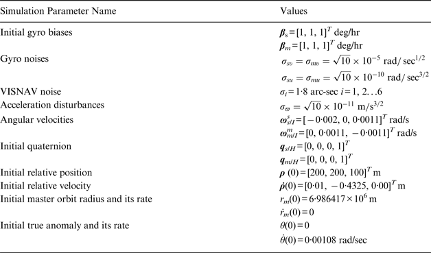
In this section, simulations are performed to estimate relative quaternions, relative position, and velocity between two spacecraft, as well as the gyro biases. A summary of the true values of simulation parameters is given in Table 1, and six beacon locations are shown in Table 2. The performances of the EKF and two versions of the UKF with respect to initial condition errors are compared. The transformation parameters for the GRPs are given by a=1 and f=4. The parameters used in the UKF are given by α=0·005, β=2 and κ=3−n, where n=22. The entire simulation time is 300 minutes. For a fair comparison, the simulation results are based on 50 Monte Carlo runs.
Table 1. Simulation Parameters.
Table 2. Beacon Location in Metres.

In Kim et al. (Reference Kim, Crassidis, Cheng, Fosbury and Junkins2007) and Zhang et al. (Reference Zhang, Yang, Zhang, Cai and Qian2014), all initial variables are set to their true values, except for the gyro biases, which are set to zero. In this scenario, the attitude errors of [10°−10° 5°]T and [−10° 10° 5°]T are added into initial estimates of qs/H and qm/H for each axis, respectively. The initial gyro bias estimates for the slave and master spacecraft are set to zero. The 1σ errors are added into the initial relative position and velocity, radius and radial rate as well as the true anomaly and rate. The initial covariance matrix is diagonal. The three attitude error parts of the initial covariance for qs/H and qm/H are each set to one standard deviation error of 10°, i.e., [10×(π/180)]2 rad2. The three gyro-bias parts of the initial covariance for the slave and master spacecraft are each set to 2° per hour, i.e.,  $\left[ {2 \times \left( {{\pi / {(180 \times 3600)}}} \right)} \right]^2 \left( {{\rm rad/s}} \right)^2 $. The relative position and velocity parts of the initial covariance are each set to 5 m2 and 0·02 (m/s)2, respectively. The master's radius and radial rate parts of the initial covariance are each set to 1000 m2 and 0·01(m/s)2, respectively. The master's true anomaly and rate parts of the initial covariance are set to 1×10⁻⁴rad2 and 1×10⁻⁴(rad/s)2, respectively.
The performances of the EKF and two versions of the UKF are compared in Figures 2–9. Figures 2 and 3 show the roll, pitch and yaw errors for qs/H and qm/H, respectively. As can be seen, two versions of the UKF attitude estimation errors do converge to within their respective 3σ bounds within 300 minutes, whereas the EKF attitude estimation errors do not converge to within their respective 3σ bounds. Figures 4 and 5 show the norms of relative position and velocity errors, respectively. It is seen that the EKF does not produce acceptable performance, which indicates the first-order approximation cannot capture the initial condition errors. However, the designed UKF is working properly. The norms of relative position and velocity estimated errors are within 0·03 m and 3×10⁻⁵ m/s. From the partial enlargement drawings, we can see that the UKF2 is a little superior than the UKF1, which agrees well with the previous analysis. Figures 6 and 7 show the norms of slave and master gyro bias errors, respectively. It can also be seen that the UKF2 performs a bit better than the UKF1. A plot of the norm of relative attitude errors is shown in Figure 8. The relative attitude between the slave and master spacecraft is estimated by using Equation (38). As shown, both UKF1 and UKF2 can reach the norm of relative attitude errors of less than 0·05° within 300 minutes, whereas the EKF does not converge. Figure 9 shows the master orbital element errors of the UKF1 and UKF2, and the results of the EKF are not shown because it fails to converge.
Figure 2. Attitude estimated errors for qs/H and 3σ bounds.
Figure. 3. Attitude estimated errors for qm/H and 3σ bounds.
Figure 4. Norm of relative position errors.
Figure 5. Norm of relative velocity errors.
Figure 6. Norm of slave gyro bias errors.
Figure 7. Norm of master gyro bias errors.
Figure 8. Norm of relative attitude errors.
Figure 9. Master orbit element errors.
7. CONCLUSIONS
In this paper, a novel navigation approach based on an Unscented Kalman Filter has been derived to estimate the relative attitude and position between slave and master spacecraft. Our approach is to additionally estimate the attitudes of both spacecraft relative to the master's LVLH frame, so that the simplified assumption that the master's body frame coincides with its LVLH frame is removed. The general relative equations of motion for eccentric orbits are used to describe the positional dynamics. In the UKF design, an unconstrained three-component vector of Generalized Rodrigues Parameters is employed to maintain the quaternion normalization constraint. Besides the traditional UKF, a modified version of the UKF is also presented. An averaging-quaternion algorithm is employed to average a set of weighted propagated sigma-point quaternions, and then the mean of these sigma-point quaternions is used for the reference quaternion instead of the sigma-point quaternion at the centre. The performances of the EKF and two versions of the UKF with respect to initial condition errors are compared. Simulation results indicate that the proposed filters can provide more accurate estimates for relative attitude and position than the Extended Kalman Filter. The modified UKF performs a little better than the traditional UKF.
ACKNOWLEDGMENT
This work was supported by Innovation Fund of Graduate Program of National University of Defense Technology (B130105) and Scientific Research Fund of Graduate Program of Hunan Province (CX2013B004).