


1. INTRODUCTION
Localisation technologies and location-based applications have been extensively investigated in recent years. Global Navigation Satellites Systems (GNSS) have been widely adopted for positioning and navigation in outdoor scenarios. Indoor environments, on the other hand, bring about more location-based services opportunities as well as more challenges for localisation because of less availability of navigation satellites and complicated built structures hindering signal propagation.
Other than GNSS, short-ranged signals such as WiFi, Bluetooth (Bahl and Padmanabhan, Reference Bahl and Padmanabhan2000; Chen et al., Reference Chen, Pei, Kuusniemi, Chen, Kröger and Chen2013; Gomes and Sarmento, Reference Gomes and Sarmento2009; Pei et al., Reference Pei, Chen, Liu, Kuusniemi, Tenhunen and Chen2010b; Pei et al., Reference Pei, Chen, Liu, Tenhunen, Kuusniemi and Chen2010c; Priyantha et al., Reference Priyantha, Chakraborty and Balakrishnan2000), Radio-Frequency Identification (RFID) (Ni et al., Reference Ni, Liu, Lau and Patil2004), Ultra Wideband (UWB) (Pahlavan et al., Reference Pahlavan, Akgul, Heidari, Hatami, Elwell and Tingley2006), long-ranged signals such as Global System for Mobile communications (GSM) (Syrjärinne, Reference Syrjärinne2001), Digital Television (DTV) (Chen et al., Reference Chen, Yang and Chen2012), and magnetic fields (Storms et al., Reference Storms, Shockley and Raquet2010) have been utilised in indoor localisation for schemes such as proximity, fingerprinting, or triangulation. Microelectromechanical Systems (MEMS) motion sensors offer the opportunity of continuous relative navigation when the localisation infrastructure is unavailable (Chen et al., Reference Chen, Chen, Chen, Kuusniemi, Wang and Fu2010; Chen et al., Reference Chen, Chen, Chen, Zhang and Chen2011a; Chen et al., Reference Chen, Pei and Chen2011b; Foxlin, Reference Foxlin2005; Indoor Atlas Ltd, 2011; Mathews et al., Reference Mathews, Macdoran and Gold2011; Pei et al., Reference Pei, Chen, Liu, Chen, Kuusniemi, Tenhunen, Kröger, Chen, Leppäkoski and Takala2010a; Pei et al., Reference Pei, Chen, Liu, Kuusniemi, Chen and Tenhunen2011; Pei et al., Reference Pei, Liu, Guinness, Chen, Kuusniemi and Chen2012; Pei et al., Reference Pei, Guinness, Chen, Liu, Kuusniemi, Chen, Chen and Kaistinen2013). The low cost camera is also a potential localisation sensor (Ruotsalainen et al., Reference Ruotsalainen, Kuusniemi and Chen2011). Furthermore, hybrid solutions (Kuusniemi et al., Reference Kuusniemi, Liu, Pei, Chen, Chen and Chen2012; Liu et al., Reference Liu, Chen, Pei, Chen, Tenhunen, Kuusniemi, Kröger and Chen2010; Liu et al., Reference Liu, Chen, Chen, Pei and Chen2012a; Liu et al., Reference Liu, Chen, Pei, Guinness and Kuusniemi2012b) are adopted to improve the availability and reliability of localisation.
Today, the small-scale linear microphone arrays widely installed on smartphones could be used for localisation. Although the microphones involved in a small-scale array are physically located in one single device of a portable size that is easy to carry, their small scale poses major challenges to the existing localisation technologies. While large-scale microphone arrays have been widely applied for localisation (Filonenko et al., Reference Filonenko, Cullen and Carswell2010; Filonenko et al., Reference Filonenko, Cullen and Carswell2012; Hoflinger et al., Reference Hoflinger, Zhang, Hoppe, Bannoura, Reindl, Wendeberg and Schindelhauer2012; Holm, Reference Holm2012; Janson et al., Reference Janson, Schindelhauer and Wendeberg2010; Pertila et al., Reference Pertila, Mieskolainen and Hamalainen2012), small-scale linear microphones are mainly used for discriminating sounds based on direction, locating sound sources in terms of direction, and enhancing the microphone performance by reducing noises. For instance, microphone arrays have been used for scream and gunshot detection and localisation (Valenzise et al., Reference Valenzise, Gerosa, Tagliasacchi, Antonacci and Sarti2007), for monitoring vehicles, e.g. airplane, vessel, auto, etc., for noise diagnosing (Michel and Barsikow, Reference Michel and Barsikow2003; Piet et al., Reference Piet, Michel and Böhning2002; Schulte-Werning et al., Reference Schulte-Werning, Jäger, Strube and Willenbrink2003), noise reduction, speech recognition, teleconference, speaker tracking (Khalil et al., Reference Khalil, Jullien and Gilloire1994), and for game consoles, etc. However, the possibility of localisation using a small-scale array is much less explored in the literature.
In this paper, we propose an indoor localisation scheme, which relies on a small-scale linear microphone array to locate a sound source based on Time Difference Of Arrival (TDOA). The proposed localisation scheme is a hybrid solution on the basis of three existing TDOA localisation methods, which are the Weighted Least-Square (WLS) method, the Multi-Dimensional Scaling-based (MDS) method and the Levenberg-Marquardt (LM) method. For the existing localisation methods, we present two findings by simulations and field tests: 1) the WLS method and the MDS method perform well only for sources located close to the perpendicular bisector of the microphone array, while the MDS method is slightly better than the WLS method, and 2) the LM method can give an initial estimate, which indicates the location for a near-field source, or the direction for a far-field source. Considering these new findings, we design a hybrid localisation scheme consisting of two stages: 1) find the initial estimate of the source using the LM method, 2) rotate the microphone array so that the source can be roughly relocated on the perpendicular bisector of the microphone array, then find the refining estimate of the location of the source using the MDS method. By this two-stage procedure, the scheme has the advantages of the existing methods and efficiently expands the feasible area of the localisation scheme using a small-scale linear microphone array. Simulations and field tests results show that the proposed scheme can achieve an average error of 0·32 m in an 8 m by 5 m area.
The rest of the paper is organised as follows. The fundamentals of a small-scale linear microphone array are described in Section 2. Section 3 introduces the TDOA approach adopted in this paper. In Section 4, we present the proposed localisation algorithms. Our experiments and results are discussed in Section 5. Finally, some concluding remarks are drawn in Section 6.
2. SMALL-SCALE LINEAR MICROPHONE ARRAY
2.1. Speed of Sound
Sound is a compression wave that travels around 342 metres per second in dry air with temperature at 20 °C. The speed of sound in conditions of various temperatures can be calculated from Hoflinger et al. (Reference Hoflinger, Zhang, Hoppe, Bannoura, Reindl, Wendeberg and Schindelhauer2012):
 $$C = 331.3 \times \sqrt {1 + T/273.15}, $$
where C is the speed of sound in m/s, and T is the temperature in °C. In contrast with electromagnetic waves, the propagation speed of sound is significantly slower, which relaxes the requirement of timing in a sound-based localisation system.
2.2. Far-field and Near-field
For a linear array, a sound may be considered to come from a far-field source as shown in Figure 1 if:
 $$\vert r\vert \gt \displaystyle{{2L^2 f} \over C},$$
where r is the distance from a sound source to the centre of the microphone array, L is the dimension of the linear microphone array, f is the frequency of the sound, and C is the speed of sound (Steinberg, Reference Steinberg1976). The near-field sound source is shown in Figure 2.

Figure 1. Far-field model.

Figure 2. Near-field model.
3. TIME DELAY ESTIMATION
3.1. TDOA
The range from the sound source to the ith microphone of the microphone array can be calculated as:
 $$r_i = Ct_i, $$
where t i is the travel time of sound from the sound source to the ith microphone. A TDOA solution does not require the synchronisation of the clock of the sound source and that of the microphone array, which reduces the system complexity.
Suppose that the three-dimensional coordinates of the sound source and the microphones are denoted as  ${\bf s} = [s_x, s_y, s_z ]^{\rm T} \in {\bf R}^3 $$ and ${\bf m}_k = [m_{x_k}, m_{y_k}, m_{z_k} ]^{\rm T} \in {\bf R}^3 $, respectively. Then the ideal TDOA associated with the ith microphone pair (mi1, mi2) is computed as (Brandstein, Reference Brandstein1995):
 $$\Delta t_i = \displaystyle{{\Delta r_i} \over C} = \displaystyle{{\Vert {\bf s} - {\bf m}_{i1} \Vert - \Vert{\bf s} - {\bf m}_{i2} \Vert} \over C},$$
where  $\Vert \cdot \Vert$ denotes the Euclidian distance between two points. Δr i is the range difference between distance ||s− mi1|| and ||s− mi2||. Equation (4) indicates that we can solve the unknown location of a sound source with TDOA measurements of at least three independent microphone pairs.
3.2. Time Delay Estimation
Considering that in practice the TDOA estimate is a non-ideal measurement around the ideal TDOA, we formulate the Time Delay Estimation (TDE) from Equation (4) as:
 $$\Delta \hat t_i = \displaystyle{{\Vert{\bf s} - {\bf m}_{i1} \Vert - \Vert{\bf s} - {\bf m}_{i2} \Vert} \over C} + \eta _i, $$
where η i is an additive error assumed to be independently distributed for different microphone pairs.
The microphone signals at the ith and the jth microphones can be respectively modelled as:
 $$\left\{ {\matrix{ {x_i (t) = s(t) + n_i (t)} \hfill \cr {x_j (t) = s(t + \Delta t_{ij} ) + n_j (y)} \hfill \cr},} \right.$$
where s(t) is the source signal, n i(t) and n j(t) represent the additive noises respectively at the ith and the jth microphones, Δt ij denotes the time delay between two received signals. The aim of TDE is to estimate Δt ij that is proportional to the range difference (Brandstein and Ward, Reference Brandstein and Ward2001; Carter, Reference Carter1987; Knapp and Carter, Reference Knapp and Carter1976). The time domain cross-correlation method obtains the delay estimate between two microphones as the time lag that maximizes the cross-correlation between the received signals. The frequency domain algorithms based on the Generalised Cross-Correlation (GCC) method implement a frequency domain cross-correlation by introducing a weighting function to eliminate noise disturbances:
 $$R_{x1x2} (\tau ) \equiv \displaystyle{1 \over {2\pi}} \int_{ - \infty} ^\infty {W(\omega )} X_1 (\omega )X_2^{\ast} (\omega )e^{\,j\omega \tau} {\rm d}\omega, $$
where X 1(ω), X 2(ω) are the Fourier transforms of two microphone signals. X 2*(ω) is the conjugate function of X 2(ω). The Maximum Likelihood (ML) approach and the Phase Transform (PHAT) weighting functions are two widely used functions. The ML approach performs well in moderately noisy and non-reverberant environments (DiBiase et al., Reference DiBiase, Silverman and Brandstein2001; Ianniello, Reference Ianniello1982). In environments with high reverberations, the PHAT weighting function (Knapp and Carter, Reference Knapp and Carter1976), shown in Equation (8), has more robust performance:
 $$W_{PHAT} (\omega ) = \displaystyle{1 \over {\vert X_i (\omega )X_j^{\ast} (\omega )\vert}}.$$
4. LOCALISATION ALGORITHMS
In this section, firstly we address the problem of sound localisation based on the TDOA scheme. Secondly we adapt three basic localisation methods to solve the localisation problem for a linear array, namely the WLS method (Chan and Ho, Reference Chan and Ho1994), the MDS method (Wei et al., Reference Wei, Wan, Chen and Ye2008; Wei et al., Reference Wei, Peng, Wan and Chen2010), and the LM method (Lourakis, Reference Lourakis2005; Moré, Reference Moré1978; Nocedal and Wright, Reference Nocedal and Wright1999). Finally, we propose a hybrid localisation scheme to solve the localisation problem for a linear array. Our work is derived in a 2-D plane scenario, where the axis parallel to the linear array is set as the X-axis, and the perpendicular bisector of the linear array as the Y-axis. Extension to 3-D scenarios remains for future studies.
4.1. Problem Statement
The localisation problem can be formulated by over-determined non-linear equations. Given a specific speed of sound, the TDOA transforms to the range difference of arrival. Selecting the first microphone as reference, the range differences of all the possible microphone pairs with respect to the first microphone can be defined as:
 $$\Delta r_{k,1} = r_k - r_1 \equiv C\Delta t_{k,1}, \;k = 2,3, \ldots, M.$$
Taking into account the measurement error of time differences of arrival and from Equation (5), we rewrite Equation (9) as:
 $$\Delta r_{k,1} \approx C\Delta \hat t_{k,1}, \;k = 2,3, \ldots, M.$$
For convenience, we define Δr 1,1 = 0.
On the other hand, r k can be expressed as:
 $$r_k = \sqrt {(m_{x_k} - s_x )^2 + (m_{y_k} - s_y )^2}, k = 2,3, \ldots, M.$$
Then, the unknown sound source location s = [s x, sy]T should be the best approximate solution to the following set of non-linear equations:
 $$\eqalign{&\sqrt {(m_{x_k} - s_x )^2 + (m_{y_k} - s_y )^2} - \sqrt {(m_{x_1} - s_x )^2 + (m_{y_1} - s_y )^2} = C\Delta \hat t_{k,1}, \; \cr & \qquad k = 2,3, \ldots, M.}$$
4.2. Basic Localisation Algorithms
We consider three basic methods, i.e., the WLS method, the MDS method and the LM method to solve the localisation problem. The detailed algorithms of the three methods are shown as Algorithms 1, 2, and 3, respectively. While Algorithm 1 is a direct application of existing literature, Algorithms 2 and 3 are particularly modified from existing literature to adapt to the usage of the linear array. Also, Algorithms 1 and 2 are closed-form solutions, and Algorithm 3 is an iterative solution. Some remarks are shown at the end of the algorithms. The simulation results and further discussion are presented in Section 5.
Algorithm 1. The WLS method (application of Chan and Ho (Reference Chan and Ho1994))
1:  $\rho _k^2 = m_{{x_k}}^2 + m_{{y_k}}^2 $, k = 1, 2, …, M.
2:  ${x_{k,1}} = {m_{{x_k}}} - {m_{{x_1}}}$, k = 2, …, M.
3:  ${\bf Q} = \left[ {\matrix{ 1 & {0.5} & \cdots & {0.5} \cr {0.5} & 1 & \cdots & {0.5} \cr \vdots & \vdots & \ddots & \vdots \cr {0.5} & {0.5} & \cdots & 1 \cr}} \right]_{(M - 1) \times (M - 1)} $.
4:  ${\bf h} = \displaystyle{1 \over 2}\left[ {\matrix{ {\Delta r_{2,1}^2 - \rho _2^2 + \rho _1^2} \cr {\Delta r_{3,1}^2 - \rho _3^2 + \rho _1^2} \cr \vdots \cr {\Delta r_{M,1}^2 - \rho _M^2 + \rho _1^2} \cr}} \right]$.
5:  ${\bf G} = - \left[ {\matrix{ {x_{2,1}} \hfill & {\Delta r_{2,1}} \hfill \cr {x_{3,1}} \hfill & {\Delta r_{3,1}} \hfill \cr \vdots \hfill & \vdots \hfill \cr {x_{M,1}} \hfill & {\Delta r_{M,1}} \hfill \cr}} \right]$.
6:  ${\bf x}_{\bf s}^{(1)} = [s_x^{(1)}, r_1^{(1)} ]^{\rm T} = ({\bf G}^{\rm T} {\bf Q}^{ - 1} {\bf G})^{ - 1} {\bf G}^{\rm T} {\bf Q}^{ - 1} {\bf h}$.
7:  $s_y^{(1)} = \sqrt {\left( {r_1^{(1)}} \right)^2 - \left( {s_x^{(1)}} \right)^2} $.
8:  $\eqalign{{\bf B}^{(1)} &= {\rm diag}\left\{\sqrt{\left(m_{x_2} - s_x^{(1)} \right)^2 + \left(m_{y_2} - s_y^{(1)} \right)^2}, \right. \cr &\quad \left. \sqrt{\left( {m_{x_3} - s_x^{(1)}} \right)^2 + \left(m_{y_3} - s_y^{(1)} \right)^2}, \ldots, \sqrt{\left(m_{x_M} - s_x^{(1)} \right)^2 + \left(m_{y_M} - s_y^{(1)} \right)^2} \right\}.}$
9: Σ = C2B(1)QB(1).
10:  ${\bf x}_{\bf s}^{(2)} = \left[ {s_x^{(2)}, r_1^{(2)}} \right]^{\rm T} = \left( {{\bf G}^{\rm T} {\bf \Sigma} ^{ - 1} {\bf G}} \right)^{ - 1} {\bf G}^{\rm T} {\bf \Sigma} ^{ - 1} {\bf h}$.
11:  $s_y^{(2)} = \sqrt {\left( {r_1^{(2)}} \right)^2 - \left( {s_x^{(2)}} \right)^2} $.
12: The result  $\left[ {s_x, s_y} \right]^{\rm T} = \left[ {s_x^{(2)}, s_y^{(2)}} \right]^{\rm T} $ is the best approximate solution in this method.
Algorithm 2. The MDS method (modified from Wei et al. (Reference Wei, Wan, Chen and Ye2008))
1:  ${{\bf z}_k} = {[{m_{{x_k}}},{m_{{y_k}}},i \cdot \Delta {r_{k,1}}]^{\rm T}}$, k = 1, 2, …, M, i 2 = 1.
2: Calculate the (M + 1) × (M + 1) matrix D, whose (m + 1, n + 1)th entry is:
 $$[{\bf D}]_{m + 1,n + 1} = ({\bf z}_m - {\bf z}_n )^{\rm T} \cdot ({\bf z}_m - {\bf z}_n ) = (m_{x_m} - m_{x_n} )^2 + (m_{y_m} - m_{y_n} )^2 - (\Delta r_{m,1} - \Delta r_{n,1} )^2, \,m,n = 1, \ldots, M$$
The entries in the first column and the first row of D are all set to zero.
3:  ${\bf J}_{M + 1} = {\bf I}_{M + 1} - \displaystyle{1 \over {M + 1}}{\bf 1}_{M + 1} {\bf 1}_{M + 1}^{\rm T} $, where 1M+1 is a (M + 1) dimensional column vector with all elements 1.
4:  ${\bf B} = - \displaystyle{1 \over 2}{\bf J}_{M + 1} {\bf DJ}_{M + 1} $.
5: Find the eigenvalue decomposition of B, B = UΛUT, where Λ = diag{λ 1, …, λ M+1}, λ 1≥…≥λ M+1 ≥ 0, U = [u1, …, uM+1], UUT = I.
6: Un = [u4, …, um+1].
7:  ${\bf P} = \left[ {\matrix{ { - \displaystyle{1 \over {M + 1}}\sum\limits_{k = 1}^M {m_{x_k}}} & { - \displaystyle{1 \over {M + 1}}\sum\limits_{k = 1}^M {m_{y_k}}} & { - \displaystyle{1 \over {M + 1}}\sum\limits_{k = 1}^M {\Delta r_{k,1}}} \cr {m_{x_1} - \displaystyle{1 \over {M + 1}}\sum\limits_{k = 1}^M {m_{x_k}}} & {m_{y_1} - \displaystyle{1 \over {M + 1}}\sum\limits_{k = 1}^M {m_{y_k}}} & {\Delta r_{1,1} - \displaystyle{1 \over {M + 1}}\sum\limits_{k = 1}^M {\Delta r_{k,1}}} \cr \vdots & \vdots & \vdots \cr {m_{y_m} - \displaystyle{1 \over {M + 1}}\sum\limits_{k = 1}^M {m_{x_k}}} & {m_{y_M} - \displaystyle{1 \over {M + 1}}\sum\limits_{k = 1}^M {m_{y_k}}} & {\Delta r_{M,1} - \displaystyle{1 \over {M + 1}}\sum\limits_{k = 1}^M {\Delta r_{k,1}}} \cr}} \right]$.
8: m = [1/(M + 1)−1, 1/(M + 1), …, 1/(M + 1)]T with (M + 1) × 1 dimensions.
9:  ${\bf z} = [s_x, \tilde s_y, - r_1 ]^{\rm T} = \displaystyle{{{\bf P}^{\rm T} {\bf U}_n {\bf U}_n^{\rm T} {\bf m}} \over {{\bf m}^{\rm T} {\bf U}_n {\bf U}_n^{\rm T} {\bf m}}}$.
10:  $s_y = m_{y_1} + \sqrt {r_1^2 - s_x^2} $.
11: The result [s x, sy]T is the best approximate solution in this method.
Remarks:
The key equation which makes Algorithm 2 valid is PTUn = zmTUn, where z = [s x, sy, −r 1]T. Since we set Y-axis as the perpendicular bisector of the linear array, all the  $${m_{{y_k}}}(k = 1,2, \ldots ,M)$ are the same. It can be observed that the second column of P is proportional to m, leading to that the second row of PTUn and zmTUn are linearly dependent. So the second element of z is forced to be a constant, which equals to $m_{y_1} $. That is to say, s y cannot be directly solved from z. Hence, Step 9 of Algorithm 2 only gives a tentative solution for s y, i.e., $\tilde s_y $. The final solution for s y is obtained in Step 10 of Algorithm 2.
Algorithm 3. The LM method (modified from Nocedal and Wright (Reference Nocedal and Wright1999))
1: Set  $\bar \Delta \gt 0$, $\Delta _0 \in (0,\bar \Delta )$, $\eta \in [0,1/4)$.
2: Initialize xs(0) = [s x(0), s y(0)]T.
3: forl = 0, 1, 2, …
4: Calculate ε (xs(l)), J(xs(l)) from Equations (13–17):
 $$\eqalign{\varepsilon _k ({\bf x}_{\bf s}^{(l)} ) =& \left( {\sqrt {(s_x^{(l)} - m_{x_k} )^2 + (s_y^{(l)} - m_{y_k} )^2} - \sqrt {(s_x^{(l)} - m_{x_1} )^2 + (s_y^{(l)} - m_{y_1} )^2}} \right) - \Delta r_{k,1}, \cr \quad & k = 2, \ldots, M}$$
 $$\eqalign{&{\bf \varepsilon} ({\bf x}_{\bf s}^{(l)} ) = \left[ {{\bf \varepsilon} _2 ({\bf x}_{\bf s}^{(l)} ),{\bf \varepsilon} _3 ({\bf x}_{\bf s}^{(l)} ), \ldots, {\bf \varepsilon} _M ({\bf x}_{\bf s}^{(l)} )} \right]^{\rm T},}$$
 $$\eqalign{\displaystyle{{\partial \varepsilon _k ({\bf x}_{\bf s}^{(l)} )} \over {\partial s_x}} =& \displaystyle{{s_x^{(l)} - m_{x_k}} \over {\sqrt {(s_x^{(l)} - m_{x_k} )^2 + (s_y^{(l)} - m_{y_k} )^2}}} - \displaystyle{{s_x^{(l)} - m_{x_1}} \over {\sqrt {(s_x^{(l)} - m_{x_1} )^2 + (s_y^{(l)} - m_{y_1} )^2}}}, \cr \quad& k = 2, \ldots, M}$$
 $$\eqalign{ \displaystyle{{\partial \varepsilon _k ({\bf x}_{\bf s}^{(l)} )} \over {\partial s_y}} = &\displaystyle{{s_y^{(l)} - m_{y_k}} \over {\sqrt {(s_x^{(l)} - m_{x_k} )^2 + (s_y^{(l)} - m_{y_k} )^2}}} - \displaystyle{{s_y^{(l)} - m_{y_1}} \over {\sqrt {(s_x^{(l)} - m_{x_1} )^2 + (s_y^{(l)} - m_{y_1} )^2}}}, \cr \quad & k = 2, \ldots, M}$$
 $${\bf J}({\bf x}_{\bf s}^{(l)} ) = \left[\matrix{\displaystyle{\partial \varepsilon_2 ({\bf x}_{\bf s}^{(l)}) \over \partial s_x} &\displaystyle{\partial \varepsilon_2 ({\bf x}_{\bf s}^{(l)}) \over \partial s_y} \cr \vdots & \vdots \cr \displaystyle{\partial \varepsilon_M ({\bf x}_{\bf s}^{(l)}) \over \partial s_x} &\displaystyle{\partial \varepsilon_M ({\bf x}_{\bf s}^{(l)}) \over \partial s_y}} \right].$$
5: Let the diagonal matrix D with non-negative entrances satisfy:
 $$[{\bf D}^2 ]_{n,n} = \left[ {{\bf J}({\bf x}_{\bf s}^{(l)} )^{\rm T} \cdot {\bf J}({\bf x}_{\bf s}^{(l)} )} \right]_{n,n}, \quad n = 1,2.$$
6: Obtain pl that (approximately) satisfies:
 $${\mathop {\min} \limits_{{\bf p} \in {\bf R}^2} m_l ({\bf p}) = f\,({\bf x}_{\bf s}^{(l)} ) + \left( {{\bf J}({\bf x}_{\bf s}^{(l)} )^{\rm T} \cdot {\bf \varepsilon} ({\bf x}_{\bf s}^{(l)} )} \right)^{\rm T} \cdot {\bf p} + \displaystyle{1 \over 2}{\bf p}^{\rm T} \cdot \left( {{\bf J}({\bf x}_{\bf s}^{(l)} )^{\rm T} \cdot {\bf J}({\bf x}_{\bf s}^{(l)} )} \right) \cdot {\bf p},\quad {\rm s}.{\rm t}.\Vert{\bf Dp}\Vert \le \Delta _l.}$$
7: Calculate f(xs(l)), f(xs(l) + pl) from Equations (13) and (18):
 $$f\,({\bf x}_{\bf s} ) = \displaystyle{1 \over 2}\sum\limits_{k = 2}^M {\varepsilon _k^2 ({\bf x}_{\bf s} )}.$$
 8:  $\rho _l = \displaystyle{{f({\bf x}_{\bf s}^{(l)} ) - f({\bf x}_{\bf s}^{(l)} + {\bf p}_l )} \over {m_l ({\bf 0}) - m_l ({\bf p}_l)}} = \displaystyle{{f({\bf x}_{\bf s}^{(l)} ) - f({\bf x}_{\bf s}^{(l)} + {\bf p}_l )} \over { - ({\bf J}({\bf x}_{\bf s}^{(l)} )^{\rm T} {\bf \varepsilon} ({\bf x}_{\bf s}^{(l)} ))^{\rm T} {\bf p}_l - \displaystyle{1 \over 2}{\bf p}_l^{\rm T} {\bf J}({\bf x}_{\bf s}^{(l)} ){\bf J}({\bf x}_{\bf s}^{(l)} ){\bf p}_l}}. $
9: If ρ l < 1/4, then  $\Delta _{l + 1} = 1/4 \cdot \Vert{\bf p}_l \Vert$.
10: If ρ l > 3/4 and ||pl|| < Δl, then Δl+1 = Δl.
11: If 1/4 ≤ ρ l ≤ 3/4, then Δl+1 = Δl.
12: If ρ l > 3/4 and ||pl|| = Δl, then  $\Delta _{l + 1} = \min (2\Delta _l, \bar \Delta )$.
13: If ρ l > η, then xs(l+1) = xs(l) + pl.
14: If ρ l ≤ η, then xs(l+1) = xs(l).
15: If one of the following conditions is satisfied, then stop iterating, and let  $\hat{\bf x}_{\bf s} = {\bf x}_{\bf s}^{(l)} $.
1) $\left\Vert {{\bf J}({\bf x}_{\bf s}^{(l)} )^{\rm T} \cdot {\bf \varepsilon} ({\bf x}_{\bf s}^{(l)} )} \right\Vert \lt {\rm th}_1 $, where th1 is a preset threshold.
2) ||pl|| < th2, where th2 is a preset threshold.
3) f(xs(l)) < th3, where th3 is a preset threshold.
4) The maximum number of iterations is reached.

16: end (for)
Remarks:
1) The detail of Step 6 of Algorithm 3 is shown in the Appendix.
2) Limited by the objective function, the result of the LM method heavily depends on the initial point.
3) The LM method works in both far-field and near-field conditions. If the sound source is a far-field source, the LM method can give an estimate of the direction of the source. If the sound source is a near-field source, the LM method can give an estimate of the location of the source. In contrast, the direction-finding algorithms, such as Multiple Signal Classification (MUSIC), work only in the far-field condition.
4.3. The Proposed Hybrid Localisation Algorithm
We propose a hybrid localisation scheme on the basis of the discussed three basic localisation methods.
Algorithm 4. The hybrid scheme
1: Use Algorithm 3 (LM) to find an initial estimate of the source location, denoted as  ${\bf x}_{\bf s}^{(1)} = [s_x^{(1)}, s_y^{(1)} ]^{\rm T} $.
2: Calculate the angle θ = angle(xs(1)). θ refers to the angle from the Y-axis to the line connecting the origin of the coordinate system and the initial estimate of the source location.
3: Rotate the microphone array around the origin point by the angle of θ, so that the source can be roughly relocated on the perpendicular bisector of the microphone array.
4: Use Algorithm 1 (WLS) or Algorithm 2 (MDS) to find a refining estimate of the source location in the new coordinate system, denoted as xs(2) = [s x(2), s y(2)]T.
5: Use the standard coordinate transform to obtain the coordinates of the refining estimate of the sound source in the original coordinate system as:
 $${\bf x}_{\bf s}^{(3)} = [s_x^{(3)}, s_y^{(3)} ]^{\rm T} = \left[ {\matrix{ {\cos \theta} & { - \sin \theta} \cr {\sin \theta} & {\cos \theta} \cr}} \right]{\bf x}_{\bf s}^{(2)}. $$
Remarks:
1) Algorithm 4 contains two stages: the initialisation stage (Steps 1 and 2) to estimate the direction of the source, and the refining solution stage (Steps 3, 4, and 5) to estimate the location of the source.
2) The purpose of Step 3 of Algorithm 4 is to adjust the posture of the microphone array so that the source is relocated close to the perpendicular bisector of the microphone array, i.e., close to the Y-axis in the new coordinate system. It will be illustrated in Section 5 that only when the source is located close to the Y-axis can it be localised accurately by Algorithms 1 and 2. It is for this reason that Step 3 of Algorithm 4 is needed.
3) Step 3 of Algorithm 4 is feasible in practice because the microphone array is a small-scale device whose posture is easy to control.
5. EXPERIMENTAL RESULTS
In this section, via simulations and field tests, we evaluate the performance of the basic localisation methods and the proposed hybrid localisation scheme discussed in Section 4. As an example of a small-scale linear microphone array, a Kinect device (Webb and Ashley, Reference Webb and Ashley2012) with four microphones arranged in a line is used in our field tests. The width of the microphone array is measured to be 0·226 m. Simulations are also conducted with the same microphone deployment adopted in our field test.
5.1. Simulation Results and Discussions
We consider a four-element microphone array in a 10 m × 10 m area. Also, we assume that the sound source and microphones are located at the same height so that the 3-D problem is simplified to a 2-D one. We place the small-scale microphone array on the line of y = 1, as shown in Figure 3. To be more specific, the coordinates of the four microphones in the linear array are (−0.113,1), (0.036,1), (0.072,1), (0.113,1), respectively.

Figure 3. Illustration of the positions of the microphone array, the sources, and the initial points for the LM method.
Firstly, we evaluate the performance of the three basic localisation methods described in Algorithms 1, 2, and 3. To illustrate that the localisation performance varies with source locations, we select 9 typical positions, the coordinates of which are (0,2), (−1,2), (2,2), (0,5), (−1,5), (2,5), (0,8), (−1,8), (2,8) as shown in Figure 3. Since the LM method needs to initialise an initial point of searching, we set four different initial points located at (0,2·5), (0,4·5), (0,6·5), (0,8·5).
In our simulations, we suppose that the estimate error η i follows an independent and identically distributed (i.i.d.) zero-mean Gaussian distribution. For each algorithm and each sound source position, 100 independent experiments are conducted. In the WLS method and the LM method, the average of the outputs from the 100 experiments is set as the final localisation result. In the MDS method, on the other hand, the median of the outputs from the 100 experiments is set as the final localisation result, so that some experiments with huge estimate errors can be excluded from the performance evaluation. Such huge estimate errors are usually caused by a nearly zero denominator in Step 9 of Algorithm 2. Suppose that the standard deviation (STD) of the assumed Gaussian distribution is 2·924 μs, which corresponds to a STD of 1 mm for the range estimation. The localisation performances of the three algorithms are shown in Figures 4 to 6.

Figure 4. Localisation performance for sources at (0,2), (−1,2), and (2,2).

Figure 5. Localisation performance for sources at (0,5), (−1,5), and (2,5).

Figure 6. Localisation performance for sources at (0,8), (−1,8), and (2,8).
From Figures 4–6, we conclude that:
1) The WLS method and the MDS method can give accurate estimates on source locations when the sound source is close to the Y-axis. The smaller the Y coordinate of the source is, the more accurate the estimated location is. The accuracy of the MDS method is better than that of the WLS method.
2) The LM method can provide accurate estimated directions of the sources. The estimated direction of the source is more accurate when the initial point lies closer to the centre of the microphone array. However, in the LM method, an accurate estimation of the exact coordinates of the source cannot be guaranteed, since the final result of the LM method depends on the choice of the initial point.
In conclusion, the WLS method and the MDS method perform well only for sources located close to the perpendicular bisector of the microphone array, while the LM method is particularly good at estimating the direction of the source. We should re-emphasise that, in contrast to the direction-finding algorithms like MUSIC which work only in the far-field condition, the LM method works in both far-field and near-field conditions.
Secondly, we evaluate the performance of the proposed hybrid localisation scheme (Algorithm 4). The details of the hybrid scheme are explained as follows. In Step 1 of Algorithm 4, the initial points for LM method are set to be (−2,2), (−1,3), (1,3), and (2,2). The estimated direction of the source is set to be the average of the four estimated directions calculated from the four initial points. In Step 3 of Algorithm 4, the MDS method is chosen to estimate the location of the source in the rotated coordinate system, since it performs a little better than the WLS method. The other simulation parameters are the same as those for Figures 4 to 6.
In Figure 7, we compare the simulation results for the WLS method and the proposed hybrid scheme. Here, we choose the WLS method as benchmark because it is a well-known TDOA-based localisation algorithm and it has a similar performance as the MDS method as can be seen from Figures 4 to 6. Additionally, in Figure 8, we display the estimate error distribution of the hybrid scheme in a given area. The estimate error is defined as the distance between the true location and the estimated location of the same source.

Figure 7. Localisation performance for sources at (0,2), (−1,2), (2,2), (0,5), (−1,5), (2,5), (0,8), (−1,8), (2,8).

Figure 8. Estimate error distribution of the hybrid scheme in a target area.
From Figures 7 and 8, we summarise the following conclusions.
1) The estimated locations by the hybrid scheme are more accurate than those by the WLS method, especially for sources located relatively far away from the Y-axis.
2) The accuracy of the estimated locations by the hybrid scheme decreases when the source goes away from the centre of the microphone array.
3) The hybrid method could achieve an average accuracy of 0·32 m in the square area marked in grey in Figure 8.
5.2. Field tests
We verify the effectiveness of the investigated localisation algorithms using field tests. A Kinect device (Webb and Ashley, Reference Webb and Ashley2012) with four microphones arranged in a line has been used in our tests. The Kinect microphone array features four microphone capsules with each channel processing 16-bit audio at a sampling rate of 16 kHz. The dimensions of the Kinect microphone array are shown in Figure 9. The distance between the left most and the right most microphones is 0.226 m. Only one microphone is placed on the left-hand side and the three other microphones are located on the right-hand side of the device. The Kinect microphone array was originally designed for beam forming (Thomas et al., Reference Thomas, Ahrens and Tashev2012). Previous research on the Kinect microphone array mainly focuses on the direction detection of a sound source instead of the exact location. In this paper, we use the Kinect for locating a sound source and estimating its coordinates.

Figure 9. The Microphone array in a Kinect.
Figure 10 shows the test setup, where a Kinect device is placed on a table near the wall and connected with a laptop via USB connection. In the test environment, as shown in Figure 11, a sound source is located on another table with the same height as the one that the Kinect device stands on. The local coordinate system defined for our tests is depicted in Figure 11.

Figure 10. Test setup.
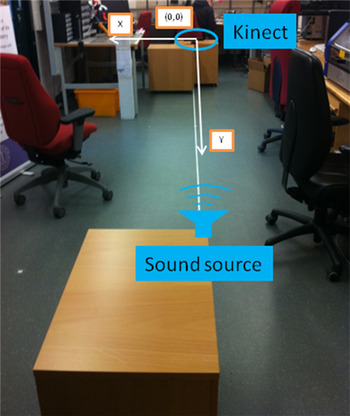
Figure 11. Test environment.
Figure 12 shows a test example in which a sound source emits a signal four times, and the signal is recorded by the four channels of a Kinect microphone array. Each channel handles the signals of one microphone. The signals are utilised for time delay estimation using the algorithms described in Section 3. It should be noted that we conducted our field tests in a simple way in order to concentrate on verifying the effectiveness of the algorithms. The more sophisticated acoustic signal processing is beyond our scope and remains for future studies.

Figure 12. Signals of Kinect's four channels.
If we consider all the possible microphone pairs, i.e., (Mic1, Mic2), (Mic1, Mic3), (Mic1, Mic4), (Mic2, Mic3), (Mic2, Mic4), (Mic3, Mic4), an example of the delay estimates is shown in Figure 13 and Table 1, where the source is located at (1,1·9). From Figure 13, we can see that both of the methods give good estimates of the true time delay, while the time domain delay estimate method is a little better than the GCC-PHAT delay estimate method. The maximum error of delay estimate is about 0·0066 ms, which is interpreted into about 2·26 mm error in the range measurement. The average deviation between the range measurement and the true range is 1·01 mm.

Figure 13. Time delay estimation experiment.
Table 1. Time Delay Estimation Experiment.

The coordinate system of the field test is the same as that used in Section 5.1. In Figure 14 and Table 2 we present the field test results of the hybrid scheme for another four sources located at (0,3), (1,2·9), (−1,4), and (1,6·7). The well-known WLS method is chosen as the benchmark.

Figure 14. Localisation performance for sources located at (0,3), (1,2·9), (−1,4), and (1,6·7).
Table 2. Localisation Error for sources located at (0,3), (1,2·9), (−1,4), and (1,6·7).

From Figure 14 and Table 2 we can see that the estimated locations by the hybrid scheme are more accurate than those of the WLS method. In the same square grey area plotted in Figure 8, the WLS method achieves an average error of 0·7834 m. The mean error of the proposed hybrid scheme is only 0·2387 m. Thus, our field tests verify the conclusions drawn in Section 5.1.
6. CONCLUSION AND FUTURE WORKS
Microphone arrays have been widely used for sound localisation. Small-scale microphone arrays have been deployed in consumer electronic devices such as Kinect and smartphones. This paper studies the possibility of using a small-scale linear microphone array for the purpose of locating a sound source. Both the time domain delay estimate method and the GCC-PHAT delay estimate method are applied to estimate the time difference of arrival in a microphone pair. Given the time difference estimations, we adapt the WLS method, the MDS method, and the LM method to calculate the coordinates of the sound source. Furthermore, we develop a hybrid scheme based on the above basic methods. Both simulations and field tests are conducted. Simulation results show that the proposed hybrid scheme outperforms the existing methods, which can achieve an average accuracy of 0·32 m in a room of 8 m by 5 m. Field tests are executed in a laboratory environment using a linear array in a Kinect device with a length of 0·226 m. The time delay estimate method is verified to be able to give delay estimates with an error less than 0·0066 milliseconds, which satisfies the requirement of localisation algorithms. Field test results corroborate the conclusions drawn from simulations.
The scope of this paper is aimed at localisation solutions. Therefore, the efficiency of the utilised algorithms is ignored. In the future, we will further study these topics, for instance, using the geometry information to constrain the iterative optimisation and restrict the search space. This paper only presents the test results for a static environment. In the future, the effects of obstacles, e.g., people, furniture, equipment etc., and tracking of moving target will be studied. Finally, we will extend our work to three-dimensional scenarios in future studies.
AKNOWLEDGEMENTS
The authors are grateful to Dr. Hongmei Hu from the Medical Physics Section of Carl von Ossietzky Universität Oldenburg, Germany for her suggestions on acoustic signal processing. The authors also would like to thank Anttoni Jaakkola from the Finnish Geodetic Institute for providing the test device. The first author would like to thank Dr. Ming Ding from National ICT Australia (NICTA) for his helpful comments.
FINANCIAL SUPPORT
This work is jointly funded by China Satellite Navigation Office and the Science and Technology Commission of Shanghai Municipality. The funding project number is BDZX005. This work is also supported by fund from the Science and Technology Commission of Shanghai Municipality (No.14511100300), the Natural Science Foundation of China (No.6140050267), and partly sponsored by Shanghai Pujiang Program (No. 14PJ1405000).
APPENDIX
The detail of Step 6 of Algorithm 3 is as follows:
Solving the minimization problem in Step 6 of Algorithm 3
6.1:  ${ \tilde {\bf J}} = {\bf J}\left( {{\bf x}_{\bf s}^{(l)}} \right) \cdot {\bf D}^{ - 1}. $
6.2:  ${\bf g} = \tilde {\bf J}^{\rm T} \cdot {\bf \varepsilon} \left( {{\bf x}_{\bf s}^{(l)}} \right).$
6.3:  ${\bf B} = \tilde{\bf J}^{\rm T} \cdot \tilde{\bf J}.$
6.4: Eigenvalue decomposition: B = QΛQT,
where Λ = diag{λ 1, λ 2}, λ 1 ≤ λ 2, QQT = QTQ = I
6.5: If λ 1 ≤ 0, then go to Step 6.7
6.6: If λ 1 > 0, then let p = − QΛ−1QTg. If ||p|| < Δl, then go to Step 6.20; if ||p|| ≥ Δl, then go to Step 6.7.
6.7: Initialise λ (n) = λ (0) which satisfies λ (0) > −λ 1.
6.8: QR decomposition:  $\left( {\matrix{ { \tilde{\bf J}} \cr {\sqrt {\lambda ^{(n)} {\bf I}}} \cr}} \right) = {\bf Q}_\lambda \left( {\matrix{ {{\bf R}_\lambda } \cr {\bf 0} \cr}} \right)$,
where Qλ is orthogonal, Rλ is upper triangular.
6.9: Solve p(λ (n)) from RλTRλp = − g.
6.10: If ||| p||−Δl| < thλ, where thλ is a preset threshold, then stop iteration and go to Step 6.20.
6.11: If ||| p||−Δl| ≥ thλ
6.12: Solve q from RλTq = p.
6.13: Set h = 1
6.14:  $\lambda ^{(n + 1)} = \lambda ^{(n)} + h \cdot \displaystyle{{\Vert{\bf p}\Vert^2} \over {\Vert{\bf q}\Vert^2}} \cdot \displaystyle{{\Vert{\bf p}\Vert - \Delta _l} \over {\Delta _l}}. $
6.15: QR decomposition:  $\left( {\matrix{ {\tilde{\bf J}} \cr {\sqrt {\lambda ^{(n+1)} {\bf I}}} \cr}} \right) = {\bf Q}_\lambda \left( {\matrix{ {{\bf R}_\lambda } \cr {\bf 0} \cr}} \right)$,
where Qλ is orthogonal, Rλ is upper triangular.
6.16: Solve p(λ (n+1)) from RλTRλp = − g.
6.17: If ||p(λ (n+1))|| < ||p(λ (n))|| and λ (n+1) > 0, then  $n \leftarrow n + 1$, go to Step 6.8.
6.18: If ||p(λ (n+1))|| < ||p(λ (n))|| and λ (n+1) ≤ 0, then let λ (n+1) = λ (n)/2, go to Step 6.8.
6.19: If ||p(λ (n+1))|| ≥ ||p(λ (n))||, then let  $h \leftarrow h/2$, go to Step 6.14.
6.20: pl = D−1p.


