1 INTRODUCTION
Global Navigation Satellite Systems (GNSS) are the primary technology today for addressing the Position, Navigation and Timing (PNT) needs of society. However, despite the global coverage that GNSS can provide, the fundamental challenge of GNSS positioning remains – good GNSS signal quality and geometry cannot be assured everywhere.
Combining GNSS with an Inertial Navigation System (INS) is an ideal way to provide a position and attitude determination solution. INS can provide all navigation information – position, velocity, acceleration and attitude – with a high update rate. However, its navigation solution drifts with time due to the sensor error accumulation. The integration with GNSS so as to calibrate the INS sensor can therefore not only mitigate one of the weaknesses of GNSS (its availability), but also bound the INS error that would accumulate with time if the INS operates in a standalone mode. This integration strategy is successful in many “open-sky” environments, but not feasible for most indoor applications. While GNSS can operate indoors, the significantly lower signal strength and severe multipath environment mean that performance is typically much worse than outdoors, and in many places there is no coverage at all. In general, with limited GNSS availability, it is hard to maintain a reliable accuracy for a few minutes even if the INS used is of high quality. Many advanced integration methods have been developed to overcome this problem, nevertheless during GNSS outages the navigation solution is unlikely to satisfy many application accuracy requirements.
To realise reliable and seamless navigation, in both outdoor and indoor environments and in the transition zone between, it is necessary to find an indoor positioning technology which can be easily incorporated into a traditional GNSS/INS integrated navigation system. “Locata” technology is a terrestrial-based system, which uses ranging signals transmitted by a number of transceivers to achieve local positioning. The transceivers are known as “LocataLites”. More than four LocataLites can form a Locata network, known as a “LocataNet”. The ranging signals transmitted by LocataLites are in the licence-free 2·4 GHz Industry, Scientific and Medical (ISM) band. When a user receiver tracks four or more Locata signals from different LocataLites, it can provide accurate positioning at centimetre-level using carrier phase measurements. Several publications are available describing the use of Locata technology for both indoor and outdoor applications (Barnes et al., Reference Barnes, Rizos, Wang, Small, Voight and Gambale2003; Reference Barnes, Rizos and Kanli2004; Choudhury et al., Reference Choudhury, Rizos and Harvey2009a; Jiang et al., Reference Jiang, Li and Rizos2014; Reference Jiang, Li and Rizos2015; Montillet et al., Reference Montillet, Roberts, Hancock, Meng, Ogundipe and Barnes2009; Rizos et al., Reference Rizos, Roberts, Barnes and Gambale2010).
A seamless indoor-outdoor navigation system based on GNSS, Locata and INS is proposed. This navigation system is expected to have good performance for both indoor and outdoor environments, and in the difficult transition zones adjacent to, or entering buildings.
As navigation sensors used for indoor environments have different operating conditions from those used outdoors, the navigation system should be designed for different modes of operation. GNSS signals are difficult to acquire and track in indoor environments, thus Locata can be used as a GNSS-alternative to integrate with INS, to assure position, velocity and attitude navigation solutions. On the other hand, in outdoor environments, all GNSS, Locata and INS measurements are available for positioning. GNSS, Locata and INS measurements can be fused to provide an improved navigation service. To satisfy the requirements of reliability and high accuracy, the Federated Kalman Filter (FKF) is adopted as the data fusion algorithm. The Locata-augmented indoor-outdoor navigation system proposed can, in principle, provide accurate and continuous navigation parameters – position, velocity and attitude – for both indoor and outdoor environments, and in the transition zone between indoors and outdoors. An indoor-outdoor experiment is carried out to evaluate the system performance.
The navigation components of the proposed indoor-outdoor navigation system and its indoor operation mode are first introduced in Section 2. The FKF algorithm and the FKF-based GNSS/Locata/INS integrated operation mode for outdoor positioning are discussed in Section 3. Finally, an indoor-outdoor experiment is described, including the system configuration and experiment design, and the test data analysis and evaluation are presented.
2 NAVIGATION COMPONENTS AND SYSTEM DESIGN
In the indoor-outdoor seamless navigation system, Locata, GNSS and INS are involved and integrated in different modes according to the implementation environments. In the indoor environment, Locata and INS integration is adopted to overcome the problem of GNSS signal obstruction.
2.1 Locata Navigation Component
LocataLite devices transmit signals at two S-band frequencies (S1 – 2·41428 GHz and S6 – 2·46543 GHz), and each LocataLite setup consists of two transmitting (Tx1 and Tx2) antennae and one receiving (Rx) antenna. Hence a cluster of four distinct signals are transmitted from each LocataLite. The frequency diversity provided by the cluster of four signals could help mitigate the cycle slip problem caused by signal interference.
2.1.1 Locata multipath-mitigation technology
Locata uses signals chipped at 10·23 MHz and the chip length is reduced to about 30 metres. This can help to eliminate the long wave multipath delays of more than two chips. However, the challenge in an indoor environment is that the short wave multipath causes less than one chip delay. To overcome the multipath problem in such challenging environments the Locata “V-Ray” antenna is used – a design based on Correlator Beam-Forming (CBF). This technique uses only one RF front-end to generate beams by sequentially switching through elements of an antenna array. Then the beam is formed with phase and gain corrections in the receiver's channel correlators. The V-Ray antenna can provide multiple beams pointing in different directions almost simultaneously (at microsecond-level switching speed).
To mitigate multipath, the formed beams must be pointed to the LocataLite transmitters. The LocataLites’ coordinates are known; thus the beam's pointing direction is dependent on the orientation of the antenna and the position of the Locata receiver. The angle-of-arrival measurements can be used to estimate the approximate rover antenna orientation and position. The receiver sweeps the beams looking for beam settings that could maximise the signal power from each LocataLite; in this way the angle-of-arrival measurements can be determined once the optimal beam settings are found.
The “V-Ray” antenna used in these tests is a basketball-sized antenna array consisting of 20 panels with 80 elements. Each panel has four elements arranged with one central and the other three on three corners to form a triangle. The space of the element between two adjacent panels is a half wavelength of the Locata signals (LaMance and Small, Reference LaMance and Small2011). The V-Ray antenna is shown in Figure 1.

Figure 1. Locata V-Ray antenna which is based on the correlator beam-forming technique to overcome the multipath effect indoors.
2.1.2 Locata mathematical model
Similar to GNSS, Locata has two types of measurements: pseudorange and carrier phase. For LocataLite channel i, the basic Locata carrier phase observation equation can be written as:
 $$\phi^i \cdot \lambda =\rho^i +\tau _{trop}^i + c \cdot \delta T + N^i \cdot \lambda +\varepsilon_{\phi}^i$$
where ϕ
i
is the Locata carrier phase measurement (in cycles), λ is the carrier signal wavelength, ρ
i
is the geometric distance between the Locata receiver and the transmitting antenna i, $\tau_{trop}^{i}$
represents the tropospheric delay, δ T is the receiver clock bias, c is the speed of light, N
i
is the Locata float carrier ambiguity and
$\tau_{trop}^{i}$
represents the tropospheric delay, δ T is the receiver clock bias, c is the speed of light, N
i
is the Locata float carrier ambiguity and $\varepsilon_{\phi}^{i}$
is the unmodelled residual errors. Due to the tight time synchronisation of the LocataLites, there is no transmitter clock error item in the observation equation.
$\varepsilon_{\phi}^{i}$
is the unmodelled residual errors. Due to the tight time synchronisation of the LocataLites, there is no transmitter clock error item in the observation equation.
The receiver clock error can be estimated via system filtering, or eliminated by differencing the measurement. In this research, the receiver clock error is eliminated by Single-Differencing (SD) the carrier phase measurements of the same frequency between two LocataLites. The tropospheric error (if present) in $\Delta \tau _{trop}^{ij}$
could be calculated by tropospheric model and many tropospheric models have been proposed in published work (Choudhury et al., Reference Choudhury, Harvey and Rizos2009b).
$\Delta \tau _{trop}^{ij}$
could be calculated by tropospheric model and many tropospheric models have been proposed in published work (Choudhury et al., Reference Choudhury, Harvey and Rizos2009b).
The SD observation equation can be written as:
 $$\Delta \phi^{ij} \cdot \lambda = (\phi^i - \phi^j) \cdot \lambda = \Delta \rho^{ij} + \Delta \tau_{trop}^{ij} + N^{ij} \cdot \lambda + v$$
where j is the reference Locata signal and i is a SD signal of the same frequency as the reference.
The unknown parameters are the Locata carrier ambiguities and the receiver's three position coordinates in the SD geometric range.
2.1.3 Ambiguity resolution
GNSS carrier ambiguities can be resolved by three methods: Known Point Initialisation (KPI), Static Initialisation (SI), or On-The-Fly (OTF) resolution. The SI needs the rover receiver to start at a known point, operating for several minutes until the estimated ambiguities converge to their likely values. As the GNSS satellites move in their orbits, the line-of-sight vectors will have obvious changes after many observation epochs, and this spatial diversity aids Ambiguity Resolution (AR). However, this approach is not suitable for Locata. In Locata applications, the LocataLites are fixed on the ground. For a stationary receiver, the ambiguities cannot be computed by solving these equations directly.
On-The-Fly-Ambiguity Resolution (OTF-AR) is also applied with enough transmitter-receiver geometry change. As the LocataLites are not moving, the OTF-AR method could be realised “kinematically” to provide the relative geometry change. The spatial diversity provided by the moving rover receiver makes Locata OTF-AR implementation possible (Jiang et al., Reference Jiang, Li and Rizos2013).
However, OTF-AR also has a limitation as the spatial diversity should be sufficiently large. Our indoor experiment was conducted in a warehouse. LocataLites were installed at the corners of the building. The distances between the Locata rover and LocataLites were short and the speed of the rover was low, hence the experimental set-up could not satisfy the OTF-AR requirements. Thus the KPI method of AR was used, based on the following expression:
 $$N^{ij} \cdot \lambda =\Delta \phi ^{ij} \cdot \lambda - \Delta \rho^{ij} - \Delta \tau_{trop}^{ij} - v$$
To obtain the accurate SD geometric distance $\Delta \rho ^{ij}$
, the initial position of the user receiver is measured by a precise survey. Standard survey techniques (Total Station if indoors and a survey-grade GNSS if outdoors) can be used to compute the initial rover coordinates.
$\Delta \rho ^{ij}$
, the initial position of the user receiver is measured by a precise survey. Standard survey techniques (Total Station if indoors and a survey-grade GNSS if outdoors) can be used to compute the initial rover coordinates.
Once the floating ambiguities are computed, they can be treated as a known item in Equation (2).
2.1.4 Locata estimation process
The Kalman Filter (KF) is adapted to process the Locata parameter estimation. The state vector of the system consists of nine parameters (three for position, three for velocity and three for acceleration). Typically, the acceleration is modelled as a white noise process – the white noise process is “isolated” in time since its value at one time is uncorrelated with that at any other time. However, the acceleration of the host vehicle (the moving platform in the proposed research) is dominated by the thrust, which has a temporal correlation. In such a case, it is appropriate to model the acceleration as a first-order Gauss Markov (GM) process rather than as a white noise process. A GM process is “local” in time as its value at one time depends on values at other time instants only through its nearest neighbours. The acceleration model is given by:
 $$\dot{a}=-\lpar {1/\tau} \rpar \cdot a + \omega _a$$
where τ is the constant correlation-time and ω a is white noise with zero-mean.
The state vector can be given as:
 $${\bf x}\lpar t \rpar = \left[ {\bf r} \quad \dot{\bf r} \quad \ddot{\bf r} \right]^{\rm T}$$
where r, $\dot{\bf {r}}$
and
$\dot{\bf {r}}$
and $\ddot{\bf {r}}$
vectors are the position, velocity and acceleration of the platform and each vector contains three components in three directions respectively.
$\ddot{\bf {r}}$
vectors are the position, velocity and acceleration of the platform and each vector contains three components in three directions respectively.
The Locata system dynamic model is:
 $${\bf x} \lpar t \rpar = {\bf F} \lpar t \rpar \cdot {\bf x} \lpar t \rpar + {\bf \omega} \lpar t \rpar $$
where ${\bf F} \lpar t \rpar = \left[\matrix{ {\bf 0}_{{\bf 3} \times {\bf 3}} \quad {\bf I}_{{\bf 3} \times {\bf 3}} \quad \quad {\bf 0}_{{\bf 3} \times {\bf 3}} \hfill \cr {\bf 0}_{{\bf 3} \times {\bf 3}} \quad {\bf 0}_{{\bf 3} \times {\bf 3}} \quad \quad {{\bf I}}_{{\bf 3} \times {\bf 3}} \hfill \cr {\bf 0}_{{\bf 3} \times {\bf 3}} \quad {\bf 0}_{{\bf 3} \times {\bf 3}} \quad -{{\bf 1} \over {\bf \rtau}} \cdot {{\bf I}}_{{\bf 3} \times {\bf 3}} } \right], {\bf \omega} \lpar t \rpar = \left[ {\bf 0}_{{\bf 1} \times {\bf 3}} \quad {\bf 0}_{{\bf 1} \times {\bf 3}} \quad \omega_{a} \quad \omega_{a} \quad \omega_{a} \right]^{\rm T}$
The measurement model is non-linear, the Extended Kalman Filter (EKF) (Kappl, Reference Kappl1971) is thus used to linearize the (non-linear) function around the prediction of the current state.
The Locata system measurement model is:
 $${\bf z}\lpar t \rpar ={{\bf H}} \lpar t \rpar \cdot {\bf x}\lpar t \rpar +{\bf \rupsilon} \lpar t \rpar $$
where the measurement vector z (t) is formed by the SD carrier phase measurements:
 $${\bf z}\left( t \right)=\left[ {\Delta \phi ^{1j}} \quad {\Delta \phi ^{2j}} \quad \cdots \hfill \quad {\Delta \phi ^{nj}} \right]^{\rm T}$$
H (t) is the observation matrix, which can be written as:
 $${\rm {\bf H}}\lpar t \rpar = \left[ \left. \matrix{ {e^1-e^j} \cr {e^2-e^j} \cr \vdots \cr {e^n-e^j}} \right| {0_{n \times 6}} \right]$$
where e* is the line-of-sight vector between receiver and satellite. ${\bf \rupsilon} \lpar t \rpar {\bf \sim} {\bf N} \lpar {\bf 0,R} \rpar$
represents the observation noise. The variance for the carrier phase measurements can be treated as the combination of transmitter location error, multipath, and measurement noise. The errors are assumed to be uncorrelated between measurements. However, the covariances of two different carrier measurements should be set as half of the carrier variance, because half of the measurements are common due to the single differencing (Amt, Reference Amt2006). The measurement covariance matrix can be written as,
${\bf \rupsilon} \lpar t \rpar {\bf \sim} {\bf N} \lpar {\bf 0,R} \rpar$
represents the observation noise. The variance for the carrier phase measurements can be treated as the combination of transmitter location error, multipath, and measurement noise. The errors are assumed to be uncorrelated between measurements. However, the covariances of two different carrier measurements should be set as half of the carrier variance, because half of the measurements are common due to the single differencing (Amt, Reference Amt2006). The measurement covariance matrix can be written as,
 $${\bf R}_{\Delta \phi} = {\sigma _{\Delta \phi}^2 \over {2}} \left[\matrix{ 2 \quad 1 \quad \cdots \quad 1 \cr 1 \quad 2 \quad \cdots \quad 1 \cr \vdots \quad \vdots \quad \ddots \quad \,\, 1 \cr 1 \quad 1 \quad \,\, 1 \quad \,\,\,\, 2 \hfill} \right]$$
where $\sigma_{\Delta \phi}^{2}$
is the noise variance of the SD carrier phase measurements.
$\sigma_{\Delta \phi}^{2}$
is the noise variance of the SD carrier phase measurements.
2.1.5 Cycle slip processing
Similar to GNSS, Locata signals also experience the problem of cycle slips and loss-of-lock due to signal interference or internal receiver tracking issues. The presence of cycle slips could cause a change of the ambiguity parameter value, which would create inconsistencies in the coordinate solution, resulting in a biased solution.
Low Signal-Noise-Ratio (SNR) values can be a useful indicator of an increased risk of cycle slips in the associated measurement, however the SNR indicator is not always reliable, because cycle slips can also occur during periods of good SNR. Another detection strategy has been developed that makes use of the typical Locata signal setup, where a group of four signals are transmitted from the same LocataLite. This method uses the Double-Differenced (DD) carrier phase measurements to detect cycle slips. The first difference is made on the raw carrier phase measurements from the Locata signal i between two subsequent epochs t 1 and t 2, to eliminate the ambiguities and any unchanged error:
 $$\Delta \phi ^i =\phi ^i (t_1 )-\phi ^i (t_2 )$$
Each LocataLite has four signals and these four come from the same or a very close location (since there are two transmit antennas, and each antenna transmits two signals), thus the second difference is made between the four signals from the same LocataLite, see Equation (12).
 $$\nabla \Delta \phi^{ij} = \Delta \phi^i - \Delta \phi^j$$
The original carrier measurements, the first differenced carrier phase measurement and the DD carrier phase measurements from one LocataLite are listed in Table 1. If there are no cycle slips, the DD carrier phase measurements would only have the receiver clock drift and other unmodelled errors, which can be assumed to have very small values (Bertsch et al., Reference Bertsch, Choudhury, Rizos and Kahle2009).
Table 1. The original, the first differenced and double-differenced carrier phase measurements for cycle slip detection.

By comparing the six DD carrier phase measurements from each LocataLite, the channel that contains the cycle slips will exceed a pre-defined threshold, here assumed to be 0·32 cycles. If all the DD carrier phase measurements that are larger than the threshold contain a specific signal, then this signal is assumed to suffer from cycle slips.
After the cycle slip is detected there are two ways to proceed: either to repair the cycle slip in the raw carrier phase measurement(s) or re-fix the ambiguities. Since Locata's cycle slips may be multiples of half cycles, which makes them harder to repair, the second approach is used. The navigation algorithm first calculates the rover's location from the assumed correct carrier phase measurements without cycle slips, then re-fixes the ambiguities with the calculated position, and finally uses the re-fixed ambiguities as known parameters in the subsequent EKF positioning estimations.
2.2 Inertial Navigation Component
Inertial navigation is a self-contained technique, which uses accelerometers and gyroscopes to measure the acceleration and rate-of-angle change, so as to determine the point displacement. The measured accelerations are integrated to obtain the user velocity and position, whereas the gyroscopes are used to maintain a reference frame and measure the angles that the coordinate axes have rotated. Three orthogonal accelerometers and three gyroscopes form an Inertial Measurement Unit (IMU). An Inertial Navigation System (INS) consists of IMU and a navigation computer which provide the user position, velocity, acceleration and attitude information by using the IMU output.
An INS can provide a Position, Velocity and Attitude (PVA) solution by integrating the measured acceleration and angular velocity. The inertial navigation mechanisation is implemented in the navigation coordinate system (n-frame) for PVA updating. The velocity and position updating is implemented by integrating the measured acceleration, whereas the attitude updates are achieved using the quaternion approach. The equations are:
 $$\eqalign{ \quad \dot{{\bf r}}^{\bf {n}} &= {\bf v}^{\bf {n}} -{\bf \romega}_{\bf {en}}^{\bf {n}} \times {\bf r}^{\bf {n}} \cr \dot{{\bf {v}}}^{{\bf n}} &= {\bf f}^{\bf {n}} +{\bf {g}}^{\bf {n}}-\lpar {\bf \romega}_{{\bf {en}}}^{\bf {n}} +{\bf 2 \romega}_{\bf {ie}}^{\bf {n}} \rpar \times {\bf v}^{\bf {n}} \cr \dot{{\bf {q}}} &= {{\bf 1} \over {\bf 2}}\left[ {\bf \romega}_{\bf nbq}^{\bf b} \right] {\bf q}}$$
where the subscripts “n”, “e”, and “i” represent the n-frame, the earth-centred-earth-fixed frame (e-frame) and Earth-centred inertial frame (i-frame), rn
and vn
refer to the position and velocity vectors respectively, $\dot{\bf {r}}^{\bf {n}}$
and
$\dot{\bf {r}}^{\bf {n}}$
and $\dot{{\bf {v}}}^{\bf {n}}$
to the position-rate and velocity-rate vectors respectively, gn
is the gravity and fn
represents the specific force sensed by the accelerometer.
$\dot{{\bf {v}}}^{\bf {n}}$
to the position-rate and velocity-rate vectors respectively, gn
is the gravity and fn
represents the specific force sensed by the accelerometer. ${\bf \romega}_{{{\bf en}}}^{\bf {n}}$
is the angular rate of the n-frame with respect to the e-frame,
${\bf \romega}_{{{\bf en}}}^{\bf {n}}$
is the angular rate of the n-frame with respect to the e-frame, ${\bf \romega}_{{{\bf ie}}}^{\bf {n}}$
is the angular rate vector of the e-frame with respect to the i-frame, q and
${\bf \romega}_{{{\bf ie}}}^{\bf {n}}$
is the angular rate vector of the e-frame with respect to the i-frame, q and $\dot{{\bf {q}}}$
refer to the attitude quaternion and its rate, respectively.
$\dot{{\bf {q}}}$
refer to the attitude quaternion and its rate, respectively. ${\bf \romega}_{{\bf nb}}^{{\bf b}}$
and its skew-symmetric matrix
${\bf \romega}_{{\bf nb}}^{{\bf b}}$
and its skew-symmetric matrix $\lsqb {{\bf \romega}_{{\bf nb}}^{{\bf b}}} \rsqb $
can be written as:
$\lsqb {{\bf \romega}_{{\bf nb}}^{{\bf b}}} \rsqb $
can be written as:
 $${\bf \romega}_{{\bf nb}}^{{\bf b}} = 0 + \omega _x i + \omega_y j + \omega _z k$$
Then,
 $$\lsqb {{\bf \romega}_{{\bf nb}}^{{\bf b}} } \rsqb =\left[ \matrix{ 0 \quad {-\omega_x } \quad {-\omega_y } \quad {-\omega_z} \cr {\omega_x } \quad 0 \quad \quad {\omega_z } \quad \,\,\, {-\omega_y } \hfill \cr {\omega_y } \,\,\, {-\omega_z } \quad \quad 0 \quad \quad {\omega_x } \hfill \cr {\omega_z } \quad {\omega_y } \quad \, {-\omega_x } \quad \quad 0 \hfill } \right]$$
The problem of inertial navigation is that its errors accumulate with time. Even if the INS initialised with proper conditions, the accuracy of the calculated position, velocity and attitude will degrade with time due to the inertial systematic errors and the non-linear nature.
2.3 Indoor Navigation Mode Based on Terrestrial and Inertial Technology
For the indoor navigation configuration of the proposed system, the Locata and INS systems are integrated with a loosely-coupled approach. The computed Locata Position and Velocity (PV) solutions are used to correct the INS PVA solutions within the system integration filtering. In addition to reducing PVA errors, the Locata PV updates are also used to converge the lever arm between IMU centre and the Locata antenna and the gyroscope and accelerometer errors. The estimated lever arm information and sensor errors are fed back to the integration filter to achieve a closed-loop update correction.
To implement the integration estimation filter, the INS error model is defined. Many INS error models have been proposed (Arshal, Reference Arshal1987; Goshen-Meskin and Bar-Itzhack, Reference Goshen-Meskin and Bar-Itzhack1992; Lee et al., Reference Lee, Lee, Rho and Park1998). The psi-angle error model is applied in this research (Goshen-Meskin and Bar-Itzhack, Reference Goshen-Meskin and Bar-Itzhack1992):
 $$\eqalign{ {\bf \rdelta} \dot{{\bf r}}^{\bf {n}} & ={{\bf \rdelta}{\bf v}}^{\bf {n}} -{\bf \romega}_{{{\bf en}}}^{\bf {n}} \times {{\bf \rdelta}{\bf r}}^{\bf {n}} \cr {{\bf \rdelta} \dot{{\bf v}}}^{\bf {n}}& = -\lpar {\bf \romega}_{{\bf ie}}^{\bf {n}} +{\bf \romega}_{{\bf in}}^{\bf {n}} \rpar \times {\bf \rdelta} {\bf v}^{\bf {n}} +{\bf \rpsi} \times {\bf f}^{\bf {n}} + \nabla^{\bf {n}} + {\bf \rdelta} {\bf g}^{\bf {n}} \cr \dot{{\bf \rpsi}} &= -{\bf \romega}_{{\bf in}}^{\bf {n}} \times {\bf \rpsi} +{\bf \rvarepsilon}^{\bf {n}} }$$
where ${\bf {\rdelta}{\bf r}}^{\bf {n}}$
,
${\bf {\rdelta}{\bf r}}^{\bf {n}}$
, ${\bf {\rdelta}{\bf v}}^{\bf {n}}$
and
${\bf {\rdelta}{\bf v}}^{\bf {n}}$
and ${\bf {\rpsi}}$
represent the position, velocity and attitude error respectively.
${\bf {\rpsi}}$
represent the position, velocity and attitude error respectively. ${\bf \romega}_{{{\bf in}}}^{\bf {n}}$
is the angular rate of the n-frame with respect to the i-frame,
${\bf \romega}_{{{\bf in}}}^{\bf {n}}$
is the angular rate of the n-frame with respect to the i-frame, $\nabla^{\bf {n}}$
is the accelerometer error,
$\nabla^{\bf {n}}$
is the accelerometer error, ${\bf {\rdelta}} {\bf g}^{\bf {n}}$
is the error of the computed gravity and
${\bf {\rdelta}} {\bf g}^{\bf {n}}$
is the error of the computed gravity and ${\bf {\rvarepsilon}}^{\bf {n}}$
is the gyroscopes’ drift error.
${\bf {\rvarepsilon}}^{\bf {n}}$
is the gyroscopes’ drift error.
The estimated state vector consists of 18 navigation error states, which can be written as three sub-vectors: ${\bf x}_{{\bf {\rpsi}{\bf rv}}}$
,
${\bf x}_{{\bf {\rpsi}{\bf rv}}}$
, ${\bf x}_{\rvarepsilon \nabla}$
and
${\bf x}_{\rvarepsilon \nabla}$
and ${\bf x}_{\bf {\reta}}$
representing the motion, sensor errors and lever arm components, respectively:
${\bf x}_{\bf {\reta}}$
representing the motion, sensor errors and lever arm components, respectively:
 $${\bf x} \lpar t \rpar = \left[ {\bf x}_{{\bf {\rpsi rv}}} \quad {\bf x}_{{\rvarepsilon \nabla}} \quad {\bf x}_{\bf {\reta}} \right]$$
Specifically:
 $${\bf x}_{\bf {\rpsi rv}} = \left[ \psi_N \quad \psi_E \quad \psi_D \quad \delta r_N \quad \delta r_E \quad \delta r_D \quad \delta v_N \quad \delta vE \quad \delta v_D \right]$$
 $${\bf x}_{{\bf {\rvarepsilon}}\nabla} = \left[ \varepsilon_x \quad \varepsilon_y \quad \varepsilon_z \quad \nabla_x \quad \nabla_y \quad \nabla_z \right]$$
 $${\bf x}_{\bf {\reta }} = \left[ \delta \eta_{Lx} \quad \delta \eta _{Ly} \quad \delta \eta_{Lz} \right]$$
where the subscripts “N”, “E”, “D” represent the north, east, and down axes in the n-frame, respectively; the subscripts “x”, “y”, “z” denote the direction of the roll, pitch, and yaw axes in the body frame, respectively; and the last six symbols $\delta \eta _{L\ast }$
represent the unknown lever arm components. The accelerometer and gyroscope errors are modelled as random biases.
$\delta \eta _{L\ast }$
represent the unknown lever arm components. The accelerometer and gyroscope errors are modelled as random biases.
The system dynamic model is:
 $$\left[ \matrix{ \dot{{\bf x}}_{\bf {\rpsi}{\bf rv}} \cr \dot{{\bf x}}_{\bf {\rvarepsilon} \nabla} \cr \dot{{\bf x}}_{\bf {\reta}} } \right] = \left[\matrix{ {\bf F}_{{\bf 11}} \quad \,\, {\bf F}_{{\bf 12}} \quad \,\, {\bf 0}_{{\bf 9} \times 3} \cr {\bf 0}_{{\bf 6} \times {\bf 9}} \quad{\bf 0}_{{\bf 6} \times {\bf 6}} \quad{\bf 0}_{{\bf 6} \times 3} \cr {\bf 0}_{3\times {\bf 9}} \quad{\bf 0}_{3\times {\bf 6}} \quad{\bf 0}_{3\times 3} \cr } \right] \left[\matrix{ {\bf x}_{\bf {\rpsi}{\bf rv}} \cr {\bf x}_{\bf {\rvarepsilon}\nabla}\cr {\bf x}_{\bf {\reta}} \cr } \right]+\left[\matrix{ {\bf 0}_{{\bf 9} \times {\bf 1}} \cr {\bf \romega}_{\bf {\rvarepsilon} \nabla} \cr {\bf 0}_{3\times {\bf 1}} } \right]$$
where the sub-matrices F11
and F12
of system matrix F are calculated based on the INS error model (Arshal, Reference Arshal1987; Goshen-Meskin and Bar-Itzhack, Reference Goshen-Meskin and Bar-Itzhack1992), ${\bf \romega}_{\bf {\rvarepsilon} \nabla}$
is the noise of accelerometer and gyroscope errors, which is modelled as random bias.
${\bf \romega}_{\bf {\rvarepsilon} \nabla}$
is the noise of accelerometer and gyroscope errors, which is modelled as random bias.
Because of the lever arm uncertainty, the Locata position and velocity should be converted to the IMU centre by using the lever arm between the two points (Li et al., Reference Li, Li, Rizos and Xu2012). The relationship between the Locata antenna and IMU centre can be represented as:
 $${\bf r}_{{{\bf Locata}}}^{\bf {n}} ={\bf r}_{{{\bf INS}}}^{\bf {n}} +{{\bf C}}_{{\bf b}}^{\bf {n}} {\bf {\reta }}^{{\bf b}}$$
 $${{\bf v}}_{{{\bf Locata}}}^{\bf {n}} ={{\bf v}}_{{{\bf INS}}}^{\bf {n}} +\lpar {{\bf \romega}_{{{\bf ie}}}^{\bf {n}} \times +{\bf \romega}_{{{\bf en}}}^{\bf {n}} \times } \rpar {{\bf C}}_{{\bf b}}^{\bf {n}} {\bf {\reta }}^{{\bf b}}-{{\bf C}}_{{\bf b}}^{\bf {n}} \lpar {{\bf {\reta }}^{{\bf b}}\times } \rpar {\bf \romega}_{{{\bf ib}}}^{{\bf b}}$$
where ${{\bf C}}_{{\bf b}}^{\bf {n}}$
is the direction cosine matrix between the body frame and the navigation frame and
${{\bf C}}_{{\bf b}}^{\bf {n}}$
is the direction cosine matrix between the body frame and the navigation frame and ${\bf \romega}_{{{\bf ib}}}^{{\bf b}}$
is the angular-rate measurement obtained from the IMU.
${\bf \romega}_{{{\bf ib}}}^{{\bf b}}$
is the angular-rate measurement obtained from the IMU.
Then the computed Locata position and velocity at the Locata antenna centre is given by:
 $$\hat{{\bf r}}_{{\bf Locata}}^{\bf {n}} = \hat{{\bf r}}_{{\bf INS}}^{\bf {n}} + \hat{{\bf C}}_{{\bf b}}^{\bf {n}} {\bf \reta}_{{\bf 0}}^{{\bf b}} - \hat{{\bf C}}_{{\bf b}}^{\bf {n}} \lpar {\bf \reta}_{{\bf 0}}^{{\bf b}} \times \rpar {\bf \rpsi} + \hat{{\bf C}}_{{\bf b}}^{\bf {n}} {\bf \rdelta \reta}^{{\bf b}}$$
 $$\hat{{\bf v}}_{{\bf Locata}}^{\bf {n}} = \hat{{\bf v}}_{{\bf INS}}^{\bf {n}} + \hat{{\bf C}}_{{\bf b}}^{\bf {n}} \left( {\bf \romega}_{{\bf ib}}^{{\bf b}} \times \right) {\bf \reta}_{{\bf 0}}^{{\bf b}} + \hat{{\bf C}}_{{\bf b}}^{\bf {n}} \left( {\bf \romega}_{{\bf ib}}^{{\bf b}} \times \right) {\bf \rdelta \reta}^{{\bf b}} - \left[ \left( \hat{{\bf C}}_{{\bf b}}^{\bf {n}} \left( {\bf \romega}_{{\bf ib}}^{{\bf b}} \times \right) {\bf \reta}_{{\bf 0}}^{{\bf b}} \right) \times \right]$$
where ${\bf {\reta}}_{\bf 0}^{{\bf b}}$
is the initial estimate of the lever arm.
${\bf {\reta}}_{\bf 0}^{{\bf b}}$
is the initial estimate of the lever arm.
Therefore, the measurement model can be written as:
 $$\matrix{ \left[ \matrix{ {\bf \rdelta}{\bf r}_{{\bf Locata}}^{\bf {n}} - {\bf \rdelta}{\bf r}_{{\bf INS}}^{\bf {n}} -{{\bf C}}_{{\bf b}}^{\bf {n}} {\bf \reta}_{{\bf 0}}^{{\bf b}} \cr {\bf \rdelta}{\bf v}_{{\bf Locata}}^{\bf {n}} - {\bf \rdelta}{\bf v}_{{\bf INS}}^{\bf {n}} -{{\bf C}}_{{\bf b}}^{\bf {n}} \left( {\bf \romega}_{{\bf ib}}^{{\bf b}} \times \right) {\bf \reta}_{{\bf 0}}^{{\bf b}} } \right] \hfill \cr \cr \quad =\left[\matrix{ \hat{{\bf C}}_{{\bf b}}^{\bf {n}} \left( {\bf \reta}_{{\bf 0}}^{{\bf b}} \times \right) \quad \quad \quad \quad {\bf I}_{{\bf 3} \times {\bf 3}} \quad {\bf 0}_{{\bf 3} \times {\bf 3}} \quad {\bf 0}_{{\bf 3} \times {\bf 6}} \quad \quad \hat{{\bf C}}_{{\bf b}}^{\bf {n}} \cr -\left[ \left( \hat{{\bf C}}_{{\bf b}}^{\bf {n}} \left( {\bf \romega}_{{\bf ib}}^{{\bf b}} \times \right) {\bf \reta}_{{\bf 0}}^{{\bf b}} \right) \times \right] \quad {\bf 0}_{{\bf 3} \times {\bf 3}} \quad {\bf I}_{{\bf 3} \times {\bf 3}} \quad {\bf 0}_{{\bf 3} \times {\bf 6}} \quad \hat{{\bf C}}_{{\bf b}}^{\bf {n}} \left( {\bf \romega}_{{\bf ib}}^{{\bf b}} \times \right) } \right] {\bf x} \left( {\bf t} \right) + {\bf \rupsilon} \left( {\bf t} \right)}$$
The measurement noise covariance in the system filtering is defined by the general accuracy of the computed Locata PV solution, which is described as:
 $${\bf R}=diag\left( {\lpar {0{\cdot}05} \rpar^2} \quad {\lpar {0{\cdot}05} \rpar^2} \quad {\lpar {0{\cdot}05} \rpar^2} \quad {\lpar {0{\cdot}1} \rpar^2} \quad {\lpar {0{\cdot}1} \rpar^2} \quad {\lpar {0{\cdot}1} \rpar^2} \right)$$
where the first three terms are the covariances of position (m 2), and the last three terms are the covariances of the velocity (m/s)2.
3 SYSTEM OPERATION IN AN OUTDOOR ENVIRONMENT
In the outdoor operation mode of the proposed system, the GNSS, Locata and INS are all able to provide navigation information, thus the best solution is to fuse the observations from the three sensors. To satisfy the requirements of high reliability and high accuracy, the FKF is adopted as the data fusion algorithm.
3.1 Federated Kalman Filtering
The FKF was developed by Carlson and Berarducci (Reference Carlson and Berarducci1994) and Carlson (Reference Carlson1996). It is typically a two-stage data processing algorithm, comprised of one master filter and a set of local filters, as described in Figure 2. The local filters obtain the measurements from independent sensors and process in parallel, then the master filter is used to fuse the obtained local estimates and yield a global solution. This decentralisation characteristic of the FKF ensures good fault detection and isolating ability and a low computation load. However, the accuracy cannot compete with conventional centralised filtering (Li, Reference Li2014; Jiang et al., Reference Jiang, Li and Rizos2015). To improve the accuracy, the information sharing approach is applied in the FKF algorithm. This approach can divide the global state prediction and the covariance across the local filters to help ensure an optimal global estimation.

Figure 2. System configuration of FKF which contains one master filter and several parallel local filters.
Suppose the dynamic equation and observation equation of the local system are:
 $${\bf x}_i \lpar k \rpar ={{\bf F}}_i \lpar k \rpar {\bf x}_i \lpar {k-1} \rpar +{\bf \romega}_i \lpar k \rpar \!, i=1,2\cdots n$$
 $${\bf z}_i \lpar k \rpar ={{\bf H}}_i \lpar k \rpar {\bf x}_i \lpar k \rpar +{{\bf v}}_i \lpar k \rpar \!, i=1,2\cdots n$$
where both ${\bf \romega}_{i}\!\lpar k\rpar $
and v
i
(k) are assumed to be zero-mean white Gaussian noises, and the covariance matrix are Q
i
(k) and R
i
(k), respectively.
${\bf \romega}_{i}\!\lpar k\rpar $
and v
i
(k) are assumed to be zero-mean white Gaussian noises, and the covariance matrix are Q
i
(k) and R
i
(k), respectively.
If the local filter and the master filter are statistically independent, they can be combined to yield the global estimates using the following information equations, where inverse covariance is the “information matrix”:
 $$\hat{{\bf {P}}}_f^{-1} =\sum\limits_{i=1}^n {\hat{{\bf {P}}}_i^{-1} } + \hat{{\bf P}}_m^{-1}$$
 $$\hat{{\bf {P}}}_f^{-1} \hat{{\bf {x}}}_f =\sum\limits_{i=1}^n {\hat{{\bf {P}}}_i^{-1} \hat{{\bf {x}}}_i} + \hat{{\bf {P}}}_m^{-1} \hat{{\bf {x}}}_m$$
where the subscript “i”, “m”, and “f\!” denote the local filter, master filter and full filter, respectively.
For the typical FKF, the local filters and the master filter share the same system model (Carlson and Berarducci, Reference Carlson and Berarducci1994; Carlson, Reference Carlson1996). Thus the master filter and local filters’ estimates are correlated because they use a common dynamic system. To eliminate the correlation, the covariance of state error and process noise are set to their upper bounds:
 $$\left\{ \matrix{ \hat{{\bf x}}_i \lpar k \rpar = \hat{{\bf {x}}}_f \lpar k \rpar \cr {\bf F}_i \lpar k \rpar = {\bf F} \lpar k \rpar } \right. \quad i=1,2\cdots n,m $$
 $$\left\{ \matrix{ {\hat{{\bf {P}}}_i^{-1} \lpar k \rpar =\hat{{\bf {P}}}_f^{-1} \beta _i } \cr {{{\bf Q}}_i^{-1} \lpar k \rpar ={{\bf Q}}_f^{-1} \beta _i }} \right. \quad i=1,2\cdots n,m $$
where $\beta _{i} \lpar >0 \rpar $
is the information-sharing factor and it satisfies the condition:
$\beta _{i} \lpar >0 \rpar $
is the information-sharing factor and it satisfies the condition:
 $$\sum\limits_{i=1}^{n,m} {\beta _i} = 1$$
According to the general KF updating process, the time updating is executed for both local filters and master filter:
 $$\hat{{\bf {P}}}_i \lpar {k\vert k-1} \rpar = {{\bf F}}_i \lpar k \rpar \hat{{\bf {P}}}_i \lpar {k-1} \rpar {{\bf F}}_i^T \lpar k \rpar +{{\bf Q}}_i \lpar k \rpar ; \quad i=1,2\cdots n,m$$
 $$\hat{{\bf {x}}}_i \lpar {k\vert k-1} \rpar = {{\bf F}}_i \lpar k \rpar \hat{{\bf {x}}}_i \lpar {k-1} \rpar ; \quad i=1,2\cdots n,m $$
As for the measurement propagation, local filters and the master filter are different:
 $${{\bf K}}_i \lpar k \rpar =\hat{{\bf {P}}}_i \lpar {k\vert k-1} \rpar {{\bf H}}_i^T \lpar k \rpar \left[ {{{\bf H}}_i \lpar k \rpar \hat{{\bf {P}}}_i \lpar {k\vert k-1} \rpar {{\bf H}}_i^T \lpar k \rpar +{\bf R}_i \lpar k \rpar } \right] ^{-{{\bf 1}}}; \quad i=1,2\cdots n$$
 $$\hat{{\bf {P}}}_i \lpar k \rpar = \left[ {{{\bf I}}-{{\bf K}}_i \lpar k \rpar {{\bf H}}_i \lpar k \rpar } \right] \hat{{\bf {P}}}_i \lpar {k\vert k-1} \rpar ; \quad i=1,2\cdots n $$
 $$\hat{{\bf {x}}}_i \lpar k \rpar =\hat{{\bf {x}}}_i \lpar {k\vert k-1} \rpar +{{\bf K}}_i \lpar k \rpar \lsqb {{\bf z}_i \lpar k \rpar -{{\bf H}}_i \lpar k \rpar \hat{{\bf {x}}}_i \lpar {k\vert k-1} \rpar } \rsqb ; \quad i=1,2\cdots n $$
 $$\hat{{\bf {P}}}_m \lpar k \rpar =\hat{{\bf {P}}}_m \lpar {k\vert k-1} \rpar $$
 $$\hat{{\bf {x}}}_m \lpar k \rpar = \hat{{\bf {x}}}_m \lpar {k\vert k-1} \rpar $$
The fusion algorithm can be applied to combine the above local and master results:
 $$\hat{{\bf {P}}}_f^{-1} \lpar k \rpar =\hat{{\bf {P}}}_m^{-1} \lpar k \rpar +\sum\limits_{i=1}^n {\hat{{\bf {P}}}_i^{-1} } \lpar k \rpar$$
 $$\hat{{\bf {x}}}\lpar k \rpar =\hat{{\bf {P}}}_f \lpar k \rpar \left[ {\hat{{\bf {P}}}_m^{-1} \lpar k \rpar \hat{{\bf {x}}}_m \lpar k \rpar +\sum\limits_{i=1}^n {\hat{{\bf {P}}}_i^{-1} \lpar k \rpar \hat{{\bf {x}}}_i \lpar k \rpar } } \right]$$
Then the correct global estimates are obtained.
3.2 FKF-based GNSS/Locata/INS Hybrid System
For a GNSS/Locata/INS hybrid system, both Locata and GNSS can provide independent position and velocity solutions. The two sets of position and velocity solutions are combined with INS sensor output separately to construct the measurements of the two local systems. As the measurements of the two local filters include INS information, and the two local filters apply the INS navigation model, the two local filters are correlated. The information-sharing factor-based FKF algorithm is thus applied. Both Locata/INS and GNSS/INS local filters estimate the nine motion parameters, INS sensor error and corresponding lever arms use their own observations. As both the Locata and GNSS local filters apply the INS navigation model, the dynamic equations of the two filter systems are the same. The ith ( $i=\hbox{Locata}$
, GNSS) local filter is described by the following equations:
$i=\hbox{Locata}$
, GNSS) local filter is described by the following equations:
 $${\bf x}\lpar k \rpar ={{\bf F}}\lpar k \rpar {\bf x}\lpar {k-1} \rpar +{\bf \romega}\lpar k \rpar$$
 $${\bf z}_i \lpar k \rpar ={{\bf H}}_i \lpar k \rpar {\bf x}_i \lpar k \rpar +{{\bf v}}_i \lpar k \rpar $$
where ${\bf z}_{i} \lpar k \rpar \in {\bf R}_{i}^{m}$
is the output of the ith sub-system, H
i
(k) and v
i
(k) are the observation matrix and the observation noise of the local systems.
${\bf z}_{i} \lpar k \rpar \in {\bf R}_{i}^{m}$
is the output of the ith sub-system, H
i
(k) and v
i
(k) are the observation matrix and the observation noise of the local systems.
The estimated state vector could be written as three sub-vectors: motion component, inertial sensor errors, and lever arm components, as in Equation (17). Since the Locata and GNSS antennae are installed in different positions, the lever arm correction must be applied. As in the indoor navigation mode, both Locata and GNSS antennae positions are corrected to the IMU centre using estimated corresponding lever arms. Therefore, the lever arm component consists of six states, and the estimated state vector has 21 navigation error states in total. The lever arm component in Equation (17) can be written as:
 $${\bf x}_{\bf {\reta }} =\left[\matrix{ {\delta \eta_{Lx} } \quad {\delta \eta_{Ly} } \quad {\delta \eta_{Lz} } \quad {\delta \eta_{Gx} } \quad {\delta \eta_{Gy} } \quad {\delta \eta_{Gz} } } \right]$$
Then the system dynamic model is of the same form as Equation (21), rewritten as below:
 $$\left[\matrix{ \dot{{\bf {x}}}_{\bf {\rpsi}{\bf rv}} \cr \dot{{\bf {x}}}_{\bf {\rvarepsilon}\nabla} \cr \dot{{\bf {x}}}_{\bf {\reta}} \cr } \right] =\left[\matrix{ {{{\bf F}}_{{{\bf 11}}} } \quad \, {{{\bf F}}_{{{\bf 12}}}} \quad \,\, {{\bf 0}_{{{\bf 9}}\times {{\bf 6}}} } \cr {{\bf 0}_{{{\bf 6}}\times {{\bf 9}}} } \quad {{\bf 0}_{{{\bf 6}}\times {{\bf 6}}} } \quad {{\bf 0}_{{{\bf 6}}\times {{\bf 6}}} } \cr {{\bf 0}_{{{\bf 6}}\times {{\bf 9}}} } \quad {{\bf 0}_{{{\bf 6}}\times {{\bf 6}}} } \quad {{\bf 0}_{{{\bf 6}}\times {{\bf 6}}} } \cr } \right]\left[\matrix{ {{\bf x}_{{\bf {\rpsi}{\bf rv}}}} \cr {{\bf x}_{{\bf {\rvarepsilon}}\nabla}} \cr {{\bf x}_{\bf {\reta}}} \cr } \right] + \left[\matrix{ {{\bf 0}_{{{\bf 9}}\times {{\bf 1}}}} \cr {{\bf \romega}_{{\bf {\rvarepsilon}} \nabla}} \cr {{\bf 0}_{{{\bf 6}}\times {{\bf 1}}}} } \right]$$
The linearized measurement equations of the Locata and GNSS local filters are given by:
 $$\matrix{ \left[\matrix{ {{\bf \rdelta}{\bf r}}_{{\bf L}}^{\bf {n}} - {{\bf \rdelta}{\bf r}}_{{{\bf INS}}}^{\bf {n}} -{{\bf C}}_{{\bf b}}^{\bf {n}} {{\bf \reta }}_{{{\bf L0}}}^{{\bf b}} \cr {\bf \rdelta}{\bf v}_{{\bf L}}^{\bf {n}} - {{\bf \rdelta}{\bf v}}_{{\bf INS}}^{\bf {n}} -{{\bf C}}_{{\bf b}}^{\bf {n}} \left( {\bf \romega}_{{\bf ib}}^{{\bf b}} \times \right) {\bf \reta}_{{\bf L0}}^{{\bf b}} } \right] \hfill \cr \cr \quad = \left[ \matrix{ \hat{{{\bf C}}}_{{\bf b}}^{\bf {n}} \left( {\bf \reta}_{{\bf L0}}^{{\bf b}} \times \right) \cr -\left[ {\left( {\hat{{{\bf C}}}_{{\bf b}}^{\bf {n}} \left( {{\bf \romega}_{{{\bf ib}}}^{{\bf b}} \times } \right) {{\bf \reta }}_{{{\bf L0}}}^{{\bf b}} } \right) \times } \right] } \quad \matrix{ {\bf I}_{{\bf 3} \times {\bf 3}} \cr {\bf 0}_{{\bf 3} \times {\bf 3}}} \quad \matrix{ {\bf 0}_{{\bf 3} \times {\bf 3}} \cr {\bf I}_{{\bf 3} \times {\bf 3}}} \quad \matrix{ {\bf 0}_{{\bf 3} \times {\bf 6}} \cr {\bf 0}_{{\bf 3} \times {\bf 6}}} \quad \matrix{ \hat{{\bf C}}_{{\bf b}}^{\bf {n}} \cr \hat{{\bf C}}_{{\bf b}}^{\bf {n}} \left( {{\bf \romega}_{{{\bf ib}}}^{{\bf b}} \times } \right)} \quad \matrix{ {\bf 0}_{{\bf 3} \times {\bf 3}} \cr {\bf 0}_{{\bf 3} \times {\bf 3}}} \right] \cr \cr \quad \quad \times {\bf x}\left( t \right) +{{\bf v}}\left( t \right) \hfill}$$
 $$\matrix{ \left[\matrix{ {\bf {\rdelta r}}_{{\bf G}}^{\bf {n}} -{\bf {\rdelta r}}_{{{\bf INS}}}^{\bf {n}} -{{\bf C}}_{{\bf b}}^{\bf {n}} {\bf {\reta }}_{{{\bf G0}}}^{{\bf b}} \cr {{\bf {\rdelta} {\bf v}}_{{\bf G}}^{\bf {n}} -{\bf {\rdelta} {\bf v}}_{{{\bf INS}}}^{\bf {n}} -{{\bf C}}_{{\bf b}}^{\bf {n}} \lpar {{\bf \romega}_{{{\bf ib}}}^{{\bf b}} \times } \rpar {\bf {\reta }}_{{{\bf G0}}}^{{\bf b}}} } \right] \hfill \cr \cr \quad = \left[ \matrix{ \hat{{{\bf C}}}_{{\bf b}}^{\bf {n}} \left( {\bf \reta}_{{\bf G0}}^{{\bf b}} \times \right) \cr -\left[ {\left( {\hat{{{\bf C}}}_{{\bf b}}^{\bf {n}} \left( {{\bf \romega}_{{{\bf ib}}}^{{\bf b}} \times } \right) {{\bf \reta }}_{{{\bf G0}}}^{{\bf b}} } \right) \times } \right] } \quad \matrix{ {\bf I}_{{\bf 3} \times {\bf 3}} \cr {\bf 0}_{{\bf 3} \times {\bf 3}}} \quad \matrix{ {\bf 0}_{{\bf 3} \times {\bf 3}} \cr {\bf I}_{{\bf 3} \times {\bf 3}}} \quad \matrix{ {\bf 0}_{{\bf 3} \times {\bf 6}} \cr {\bf 0}_{{\bf 3} \times {\bf 6}}} \quad \matrix{ {\bf 0}_{{\bf 3} \times {\bf 3}} \cr {\bf 0}_{{\bf 3} \times {\bf 3}}} \quad \matrix{ \hat{{\bf C}}_{{\bf b}}^{\bf {n}} \cr \hat{{\bf C}}_{{\bf b}}^{\bf {n}} \left( {{\bf \romega}_{{{\bf ib}}}^{{\bf b}} \times } \right)} \right] \cr \cr \quad \quad \times {\bf x}\lpar t \rpar + {\bf v} \lpar t\rpar \hfill}$$
As the measurements of each local filter are the position and velocity corrections from GNSS or Locata in three directions, this means the six identical components in the matrix represent the uncertainty of position and velocity solutions from GNSS and Locata. Thus, they are defined by the local Locata and GNSS position and velocity estimation errors, the corresponding covariance is:
 $${\bf R}_{{\bf L}} = diag\left( {\lpar {0{\cdot}05} \rpar^2} \quad {\lpar {0{\cdot}05} \rpar^2} \quad {\lpar {0{\cdot}05} \rpar^2} \quad {\lpar {0{\cdot}1} \rpar^2} \quad {\lpar {0{\cdot}1} \rpar^2} \quad {\lpar {0{\cdot}1} \rpar^2} \right)$$
 $${\bf R}_{{\bf G}} =diag\left( {\lpar {0{\cdot}15} \rpar^2} \quad {\lpar {0{\cdot}15} \rpar^2} \quad {\lpar {0{\cdot}05} \rpar^2} \quad {\lpar {0{\cdot}2} \rpar^2} \quad {\lpar {0{\cdot}2} \rpar^2} \quad {\lpar {0{\cdot}2} \rpar^2} \right)$$
where the first three terms are the covariances of position (m 2), and the last three terms are the covariances of the velocity m/s 2.
4 EXPERIMENT AND RESULT ANALYSIS
The indoor-outdoor experiment was conducted at Locata Corporation's Numerella Test Facility (NTF), located in rural New South Wales, Australia. The indoor testing part was conducted in a metal warehouse, which was mostly empty apart from some furniture and tools placed near the walls. Figure 3 shows the outdoor and indoor testing environments.

Figure 3. Indoor-outdoor testing environment at NTF, the indoor testing is conducted in a metal warehouse.
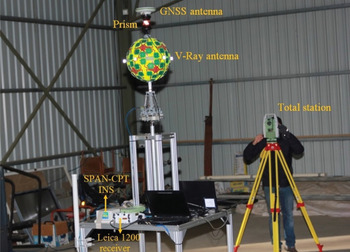
The experiment devices were installed on a testing trolley. The devices that were used in the test were one Leica 1200 dual-frequency GNSS receiver, one NovAtel SPAN-CPT GNSS/INS system which can output raw IMU measurements as well as an integrated GNSS/INS navigation solution and one Locata rover unit. The performance parameters of the inertial sensors are listed in Table 2. The Locata V-Ray antenna and the GNSS antenna were mounted on the top of trolley and the GNSS antenna was used by both the SPAN-CPT and the Leica GNSS receiver. The benchmark system was an auto-tracking Total Station (TS), which can provide position ground truth information in both indoor and outdoor environments. The TS prism was installed between the Locata V-Ray antenna and the GNSS antenna. The full experiment device setup is shown in Figure 4.

Figure 4. Experiment device set-up, including a dual-frequency GNSS receiver, a Locata user rover, an INS system and a Total Station.
Table 2. Technical parameters of the IMU.

The GNSS and Locata measurement rates were both set to 10 Hz. Global Positioning System (GPS) data was used as the GNSS local system in this research. The inertial measurement rate was set to 100 Hz and synchronised with GPS time. No changes were made to the configuration during the test.
The LocataNet comprised ten LocataLites, five of them installed inside the warehouse and the remaining five were located outside. They were time-synchronised in a cascaded mode, configured for synchronisation with respect to GPS time. The location of the LocataLites and the rover trajectory computed by integrated solution are shown in Figure 5. The green line in the plot shows the east metal wall of the warehouse, which distinguishes the indoor and outdoor environments.

Figure 5. Rover trajectory and LocataLite installation.
Unfortunately, the TS could not be satisfactorily synchronised with GNSS, Locata or INS during the tests, hence the TS observations were not available for accurate assessment of the system in kinematic mode. Hence all test result accuracy analyses were conducted for the static test points. The zoomed rover trajectory and the static test points are shown in Figure 6. The test started from point 1. The rover stayed at point 1 at the beginning and then moved to the next test point, stopping for several minutes at each point. The times and testing period for the static testing points are listed in Table 3. There were eight static points in total, with six static points inside the warehouse and the other two points placed outside.

Figure 6. Zoomed trajectory and static testing points.
Table 3. Times and testing period for the static testing points.

Figure 7 is the scatter diagram of the position differences (compared to the truth positioning solutions from the TS) for the horizontal direction components. The top left plot shows the scatter results on all eight testing points, while the top right plot and bottom plot show the indoor and outdoor testing results, respectively. The red dot indicates the origin of the coordinate system. The inner circle has a radius of 2 cm and the outer circle has a radius of 7 cm. It can be seen from top left plot that the indoor-outdoor positioning test has an overall horizontal accuracy of better than 7 cm. Comparing top right plot and bottom plot, it can be seen that the outdoor portion of the test has better positioning performance than indoors – most outdoor points are located inside the 2 cm radius circle, and the indoor points are better than 7 cm.

Figure 7. Scatter plot of results in static points; the top left plot is all static points results; the top right plot is the indoor static points results and the bottom plot is the outdoor static points results.
Figure 8 shows the filtering results of the proposed GNSS/Locata/INS integration system in north, east, and vertical directions, compared with the TS results at eight static points. It can be seen the positioning results are continuous and all at centimetre-level. The Root Mean Square (RMS) of the north, east and vertical position components are shown in Figure 9. The eight bar charts in each plot represent the data calculated at the eight static testing points. It can be seen that in both the indoor and outdoor tests the positioning accuracy are at the centimetre-level.

Figure 8. Filter results of the GNSS/Locata/INS integration system.

Figure 9. RMS of position difference for the three position components.
The Mean Radial Spherical Error (MRSE) describes the Three-Dimensional (3D) position error. The MRSE values are listed in Table 4 and plotted in Figure 10. The left plot in Figure 10 is the MRSE evaluation at each static point, and the three red bar charts in the right plot show the MRSE comparison calculated for the six indoor points, two outdoor points and all eight static points, respectively. It can be seen from the left plot that the MRSE for all eight static points is less than 5 cm. From the right plot in Figure 10 it can be seen that the MRSE of the indoor solution and outdoor solution are 0·024 cm and 0·012 cm, respectively, and the MRSE calculated for all static points is 0·021 cm, which confirms that although the proposed navigation system could achieve higher accuracy positioning outdoors, the overall positioning performance for indoor-outdoor environments is good, providing continuous and accurate 3D positioning results.

Figure 10. MRSE evaluation of each static point and comparison between indoor and outdoor environments.
Table 4. MRSE evaluation for each static point, and overall analysis for separate indoor and outdoor points.

To evaluate the performance of the triple integrated system and the local GNSS/INS and Locata/INS system, the running trajectory of the proposed indoor-outdoor multi-sensor navigation system and the local GNSS/INS and local Locata/INS integration system are compared respectively. The trajectories of the local GNSS/INS integrated system and triple integrated system are plotted in Figure 11. It can be seen that the running trajectory of the local GNSS/INS integrated system diverges far from the correct trajectory although in the outdoor part this is due to the severe GNSS signal jamming in the near-house area. The positioning accuracy could be at more than 5 m. Figure 12 shows a comparison of trajectories of the local Locata/GNSS system and GNSS/Locata/INS integration system. It can be seen that the two trajectories are almost overlapped. The zoom-in part in Figure 12 shows the positioning results of the two systems at static points 6 and 7, one can see that the positioning results computed by the triple integrated system are more concentrated on the reference points than the local Locata/INS system. It can be concluded that the trajectory of the proposed GNSS/Locata/INS integrated system is closer to the right track.

Figure 11. Computed trajectory comparison of the proposed GNSS/Locata/INS system and local GNSS/INS system.

Figure 12. Computed trajectory comparison of the proposed GNSS/Locata/INS system and local Locata/INS system.
To further analyse the performance of the proposed indoor-outdoor navigation system, the trajectories derived from the Locata-augmented system and the NovAtel SPAN-CPT GNSS/INS system are compared in Figure 13, where the blue trajectory is computed from the proposed navigation system, and the red one is from the commercial navigation system. As the GNSS signals are obstructed in indoor environments, the SPAN-CPT system cannot provide reliable trajectory information. Hence the comparison is conducted from 364,739 s onwards, that is the outdoor and (partial) indoor portion of the test. From Figure 13 one can see the trajectory of the proposed system is largely correct, while the trajectory computed by the SPAN-CPT system obviously diverges from the right track even when outside the warehouse. The reason could be that although it is outdoors, and the GNSS receiver is able to track more than four satellites, the signal quality is not as good as in an “open-sky” environment, and hence accurate positioning is not possible due to the severe multipath effect cause by the metal cladding of the warehouse.

Figure 13. Computed trajectory comparison of the proposed Locata-augmented navigation system and the NovAtel SPAN-CPT GNSS/INS system (the comparison conducted from 364,739 s onward).
Similarly, the attitude comparison between the proposed navigation system and SPAN-CPT system is plotted in Figure 14. This comparison is conducted for the whole testing period, from indoors to outdoors and finally coming back indoors again. It can be seen that the attitude results computed from the two systems indicate the same trend. From a closer analysis of the first indoor period and the outdoor period, one can see the roll and pitch results of the SPAN-CPT system have similar “oscillation” ranges. However, the indoor testing floor is flatter and smoother than the outdoor testing environment, hence the indoor roll and pitch should be more stable than in the outdoor portion of the test. The attitude result of the proposed system appears to be closer to the real movement, as the roll and pitch results of the proposed system have a smaller “oscillation” when operating indoors compared with outdoors.

Figure 14. Attitude comparison of the proposed Locata-augmented navigation system and the NovAtel SPAN-CPT GNSS/INS system.
5 CONCLUDING REMARKS
This paper described an integrated navigation system based on Locata, GNSS and INS technologies, which can be used for mixed indoor-outdoor environments to fulfil the navigation requirements. To overcome the multipath effect in indoor environments and in indoor-outdoor transition zones, the Locata V-Ray antenna is used. The proposed navigation system has two operating modes: indoor and outdoor. As indoors is a difficult GNSS signal environment, Locata is used as the GNSS-alternative to integrate with INS to deliver the PVA navigation solution. On the other hand, GNSS signals can be tracked in outdoor environments, although the observation quality in certain areas around buildings might not be as good as in the “open-sky” environment. The GNSS measurements are nevertheless useful external information that improves the system performance. The decentralised FKF is used to fuse the GNSS, Locata and INS measurements to ensure reliability and accuracy, and to provide improved navigation solutions. To evaluate the proposed navigation system, a test was conducted inside and outside a metal warehouse. The testing trolley was moved from indoors to outdoors, and finally back indoors, visiting eight static points. The test results confirmed that the proposed navigation system can provide seamless indoor-outdoor positioning solutions with a 3D accuracy better than 5 cm in all environments. Compared with a conventional GNSS/INS navigation system, the proposed indoor-outdoor navigation system has better performance in terms of positioning and attitude determination, even for outdoor areas.
ACKNOWLEDGEMENTS
The authors acknowledge the assistance of staff of the Locata Corporation for the indoor-outdoor test. This work was supported in part by the State Key Project of Chinese Ministry of Science and Technology under Grant 2016YFB1200100, State Key Program of National Natural Science Foundation of China under Grant U1334211 and 61490705, the Fundamental Research program for Central Universities under Grant 2016RC020, and Beijing Natural Science Foundation 4172049.