


1. INTRODUCTION
The accuracy needed for the Orbit Determination System (ODS) in satellites depends upon the attitude determination system accuracy and ground pixel resolution of the satellite's remote sensing payload (Gill, Reference Gill, Montenbruck and Terzibaschian2000). Therewith the acquisition capability of the ground tracking system must be considered (Kumar, Reference Kumar1981).
The goal in orbit estimation is to determine the satellite orbit that best fits or matches a set of tracking data. Tracking data or “observation” data includes any observable quantities that are a function of the position and or velocity of a satellite at a point in time. Examples include range, range rate (Doppler), azimuth and elevation from ground stations of known location (Escobal, Reference Escobal1976; Vallado, Reference Vallado2007). Other data types can include range and/or range rate from other satellites, as well as Global Positioning System (GPS) data. The GPS observations type is the position and velocity vector and the GPS observations time is continuous (Choi et al., Reference Choi, Yoon, Lee, Park and Choi2010).
The most commonly used estimation algorithm for combining sensor information with a satellite orbital model is the Kalman filter (Chobotov, Reference Chobotov2002; Chao, Reference Chao2005). The orbit dynamic models are applied to predict the orbit from a prior observation time to a new one. A key element in the Kalman filter is an accurate observation model.
In this case observation modeling is the process of modeling the forces acting on a satellite and environmental factors affecting the observation data. Good observation modeling is critical to a successful estimation of the state.
In the context of orbit determination, the perturbations are a substantial obstacle in achieving highly accurate results. The factors that act on the satellite include earth gravity, third body effects, atmospheric drag and force generated by thrusters, etc (Vallado, Reference Vallado2007). The gravity attraction is considered as the dominant force (Montenbruck and Gill, Reference Montenbruck and Gill2000). In this paper, it is demonstrated that by including the geopotential gravity, we can achieve an accurate model for orbit determination.
Orbit determination using a GPS plays an important role in generating precise orbit solutions because a GPS can provide global and continuous observable data sets to Low-Earth-Orbit (LEO) satellites (Jia and Xiong, Reference Jia and Xiong2005; Hwang et al., Reference Hwang, Lee, Kim and Kim2007; Ramos et al., Reference Ramos, Hernandez, Miguel and Sanz2007).
Continuous 3-D position measurements by GPS can reduce the OD error caused by deficiencies between the satellite orbital model and measurement data.
Due to satellite power limitations, the GPS receiver will not be operated during manoeuvres or in the imaging mode. The requirements for the onboard determination system are to provide, even when the GPS receiver has been turned off, position and velocity with proper accuracy. Accordingly, this paper presents a solution to provide the desired accuracy despite power consumption constraints. For this, the inherent advantages, disadvantages and trade-offs that are required to select the suitable duty cycle and on/off intervals are presented.
The harsh conditions in space, especially exposure to radiation, vibration and extreme changes in temperature cause fault occurrence in satellite components to be inevitable. So, limited access to the satellite and the high cost of ground facility construction make it necessary to achieve automatic fault management features in the ODS capable of fault detection and accommodation.
Today, analytical model based fault detection and isolation methods have been applied in different areas as a mature and structured field of research (Rife, Reference Rife2009). More particularly, these approaches have been used extensively for attitude control (Wu and Saif, Reference Wu and Saif2010) or attitude determination purposes (Soken and Hajiyev, Reference Soken and Hajiyev2010; Bae and Kim, Reference Bae and Kim2010). However these approaches have been applied in a limited manner in ODS and they are mostly used in applications where GPS data are fused with attitude determination sensors (Deutschman et al., Reference Deutschmann, Bar-itzhack and Harman2001; Chiang et al., Reference Chiang, Chu and Liu2001). In fact, a fault tolerant attitude determination system has been the aim in these articles. In this paper, an independent and autonomous ODS has been designed to achieve fault detection, isolation and accommodation features. Generally, model based approaches have relied on consistency tests that compare the measurements from a physical system with the information contained within the model. The resulting differences are called residuals, which are sensitive to faults occurring in the system. When an inconsistency occurs, or an estimated parameter deviates abnormally, the residuals will be different from the zero. Due to the mass and power limitations in the IUSTSAT, we have also focused on the analytical model based fault detection and isolation in the ODS. For this, the residuals generated by the Extended Kalman Filter (EKF) are analyzed to provide fault detection and isolation features. In this paper, we have also suggested a new scheme for fault accommodation. This mechanism is conducted at two levels. At the first level, after fault declaration in the main GPS, the redundant one is replaced automatically and the errors arising in velocity and position components are modified. At the second level, we have suggested an analytical solution based on the Simplified General Perturbations model 4 (SGP4) algorithm that maintains the estimation errors in an acceptable bound even after a fault in two GPS receivers. Note that, using this idea, without any GPS and after only once receiving the Two Line Elements (TLE) data, the estimation errors are kept in a suitable bound which can satisfy the image payload and Attitude Determination and Control System (ADCS) requirements (Gill et al., Reference Gill, Montenbruck and Kayal2001). SGP4 is an onboard orbit propagator based on North American Aerospace Defense Command (NORAD) two line elements that provides the position and velocity of the satellite and serves as backup for GPS and the orbit determination process (Bandyopadhyay et al., Reference Bandyopadhyay, Sharma and Adimurthy2004). This allows orbit forecasts even in the absence of GPS measurements or orbit determination problems (Gill et al., Reference Gill, Montenbruck and Kayal2001).
Note that, since the developed algorithms in this paper are intended for IUSTSAT, we were looking for an operational and straightforward method. So, in this paper, the designed EKF is utilized simultaneously for orbit determination and autonomous fault detection. This idea leads to automatic switching to the backup GPS or SGP4 algorithm in cases where the main GPS is not reliable. Moreover, it prevents additional memory or computational volume.
The structure of this paper is as follows. Section 2 provides a discussion about the satellite mission and instruments. Section 3 describes the derived satellite orbital model and the measurement models that are used in the estimation algorithm. The filtering algorithm for satellite orbit determination is detailed in section 4. In Section 5, the fault management system is described. Different simulation results are presented in section 6. Ultimately, the paper is concluded in section 7.
2. SATELLITE MISSION AND INSTRUMENTS
The IUSTSAT is scheduled for launch in 2013 into a circular orbit of 500 km altitude and 55 degree inclination. The satellite weights a total of 100 kg and consists of a semi cubic structure measuring 80×80×120 cm (W×D×H). This structure is divided into a payload platform (optical camera and scientific payload), an electronics segment, and a service element (batteries, wheels, etc). IUSTSAT is three-axis stabilized, nadir pointing in observation mode with an attitude determination accuracy ±0·5 deg, and a pointing accuracy ±0·9 deg per axis.
Position information is required in ADCS for the nadir pointing of the optical payload sensors and the S-band high-gain antenna. The accuracy of the attitude determination is 0·5 deg and attitude control is 1 deg, for which the ODS should provide the real time position data with accuracy about 100 km and 1 Hz sampling rates. A second objective stems from the optical payload system that calls for a geocoding of the image data on the flight with an accuracy of %15 swatch (Wertz and Larsen, Reference Wertz and Larsen2000), or 13·5 km at 500 km altitude. At this height, 1 deg error in the attitude control follows to 8·7 km displacement in the position of image. Therefore the prediction accuracy of ODS must be better than 4·8 km in the imaging phase.
The hardware also includes two types of GPS receivers for providing real-time orbit information and increasing the reliability of the orbit determination system. As a consequence of the limited onboard power resources, the GPS receiver will not be operated all the time. Since this type of GPS receiver does not provide access to the raw pseudo-range and phase measurements, the satellite position in the Earth Centred Inertial (ECI) frame may only be used for orbit determination. Note that, due to first use of the mentioned GPS receiver in space missions, we have considered redundancy. However if we have access to a reliable GPS receiver, it is not necessary to apply the redundancy in the developed method.
To safeguard against potential failures of the GPS-based orbit determination system, these data can alternatively be computed from the NORAD TLE and SGP4 method with a corresponding loss of precision.
3. DERIVATION OF SATELLITE ORBITAL MODEL
The orbital model that describes the satellite's position and velocity with time was constructed using forces acting on the satellite. The position and velocity can be obtained by integrating the perturbation acceleration, respectively, with respect to the position velocity at the initial epoch. The main perturbing accelerations are (Battin, Reference Battin1999):
• non-spherical gravity
• aerodynamic drag
• Third body perturbation (Sun and Moon)
• solar radiation pressure.
Figure 1 illustrates the effect of different force model perturbations on three different orbit regimes from low earth orbit to geosynchronous earth orbit (GEO) (Vetter, Reference Vetter2007). It can be seen that, in LEO satellites, the geopotential forces are dominant and the others can be neglected.

Figure 1. Effect of force model errors on satellite orbit altitudes.
3.1. Differential Equation of Orbital Motion
The general form of motion equations, including perturbations, can be expressed as follows (Curtis, Reference Curtis2010):
 $${\bf \ddot r} = - \displaystyle{\mu \over {r^3}} {\bf r} + {\bf \bar a}_{\,pr} $$
where
 is the acceleration of satellite
r is the position vector of the satellite
r is geocentric distance to satellite position
μ is the gravitational constant
āpr is the sum of the perturbing accelerations,
In the Low Earth Orbit (LEO) satellite we can simplify eq. (1) as below:
 $${\bf \ddot r} = \; - \displaystyle{\mu \over {r^3}} {\bf r} + \; {\bf \bar a}_{Geopotential}$$
The gravitational potential due to the earth can be expressed in terms of a series of spherical harmonic functions as (Curtis, Reference Curtis2010):
 $${\rm U}(r,\phi, \lambda ) = \displaystyle{\mu \over r} + \displaystyle{\mu \over r}\; \mathop \sum \limits_{n = 1}^\infty C_n^0 \; \left( {\displaystyle{{r_{eq}} \over r}} \right)^n P_n^0 (\sin \phi )$$
where, μ is the gravitational constant of the earth, r is the mean equatorial radius of the Earth, ϕ is the geocentric latitude of the satellite, λ is the geocentric east longitude of the satellite. In this expression the Ss and Cs are un-normalized harmonic coefficients of the geopotential, and the Ps are associated Legendre polynomials of degree n and order m with argument sin ϕ.
The satellite's acceleration due to the earth's gravity derived from the gradient of the potential function expressed as:
 $${\bf \bar a}_{gravity} ({\bf r},t) = \nabla \; {\rm U}({\bf r},t)$$
This acceleration vector is a combination of point mass gravity acceleration and the gravitational acceleration due to higher order nonspherical terms in the Earth's geopotential.
Regarding our considerations, the effect caused by J2 is taken into account. Therefore, the geopotential function can be reduced as follows (Sidi, Reference Sidi1997):
 $${\rm U}(r,\phi, \lambda ) = \displaystyle{\mu \over r} - \displaystyle{\mu \over r}\; \displaystyle{{J_2} \over 2}\left( {\displaystyle{{r_{eq}} \over r}} \right)^2 \; (3\sin ^2 \phi - 1)$$
where J 2=1082·68×10−6. Consequently, the partial derivative of geopotential function is expressed as follows
 $$\dot x_1 = v_x = \; x_4 $$
 $$\dot x_2 = v_y = \; x_5 $$
 $$\dot x_3 = v_z = \; x_6 $$
 $$\eqalign{ \dot x_4 = - \mu \displaystyle{{r_x} \over {{ \| r\|}^3}} \left[ {1 + \displaystyle{3 \over 2}\; \displaystyle{{J_{2\;} r_{eq}^2} \over {{\|r\|}^2}} \left( {1 - \displaystyle{{5\; r_z^2} \over {{ \|r\|}^2}}} \right)} \right] \cr \dot x_5 = - \mu \displaystyle{{r_y} \over {{\| r\|}^3}} \left[ {1 + \displaystyle{3 \over 2}\; \displaystyle{{J_{2\;} r_{eq}^2} \over {{\| r\|}^2}} \left( {1 - \displaystyle{{5\; r_z^2} \over {{\| r\|}^2}}} \right)} \right] \cr \dot x_6 = - \mu \displaystyle{{r_z} \over {{\| r\|}^3}} \left[ {1 + \displaystyle{3 \over 2}\; \displaystyle{{J_{2\;} r_{eq}^2} \over {{\| r\|}^2}} \left( {3 - \displaystyle{{5\; r_z^2} \over {{ \|r\|}^2}}} \right)} \right]} $$
In the above equation x 1(r x), x 2(r y), x 3(r z) are the rectangular components of the position vector and x 4(v x), x 5(v y), x 6(v z) are the rectangular components of the velocity vector. The acceleration vector contributions due to J 3 are given by
 $$\eqalign{ & a_{x_{J_{3}}} = - \displaystyle{5 \over 2}\; \displaystyle{{J_3 \mu r_{eq}^3 r_x} \over {\|r\|^7}} \left( {3 r_z - \displaystyle{{7 r_z^3} \over {\|r\|^2}}} \right) \cr & a_{y_{J_{3}}} = - \displaystyle{5 \over 2} \displaystyle{{J_3 \mu r_{eq}^3 r_y} \over {\|r\|^7}} \left( {3 r_z - \displaystyle{{7 r_z^3} \over {\|r\|^2}}} \right) \cr & a_{z_{J_{3}}} = - \displaystyle{5 \over 2} \displaystyle{{J_3 \mu r_{eq}^3 } \over {\|r\|^7}} \left( {6 r_z^2 - \displaystyle{{7 r_z^4} \over {\|r\|^2}} - \displaystyle{3 \over 5} \|r\|^2} \right)} $$
The acceleration vector contributions due to J 4 are given by
 $$\eqalign{ & a_{x_{J_{4}}} = \displaystyle{{15} \over 8} \displaystyle{{J_4 \mu r_{eq}^4 \; r_x} \over {{\| r\|}^7}} \left( {1 - \displaystyle{{14 r_z^2} \over {{\| r\|}^2}} + \displaystyle{{21 r_z^4} \over {{\| r\|}^4}}} \right) \cr & a_{y_{J4}} = \displaystyle{{15} \over 8} \displaystyle{{J_4 \mu r_{eq}^4 r_y} \over {{\| r\|}^7}} \left( {1 - \displaystyle{{14 r_z^2} \over {{\| r\|}^2}} + \displaystyle{{21 r_z^4} \over {{\| r\|}^4}}} \right) \cr & a_{z_{J_{4}}} = \displaystyle{{15} \over 8} \displaystyle{{J_4 \mu r_{eq}^4 r_z} \over {{\| r\|}^7}} \left( {5 - \displaystyle{{70 r_z^2} \over {3 {\| r\|}^2}} + \displaystyle{{21 r_z^4} \over {{\| r\|}^4}}} \right)} $$
3.2. SGP4 Propagation Theory
The basis of satellite orbital propagation is Keplerian orbit elements. These parameters can be used to generate a rough estimation of a satellite's position; however, such predictions will fail to reflect reality for extended periods due to disturbances, known as perturbations, in the orbit. The need for accurate orbital prediction at the dawn of the space age led to the development of the Simplified General Perturbations model in 1970. This model was later improved into Simplified General Perturbations model 4 (SGP4) in 1980 (Hoots and Roehrich, Reference Hoots and Roehrich1980).
The SGP4 is a mathematical model, which calculates orbital state vectors of satellites and space debris relative to the Earth-centered inertial coordinate system. The SGP4 model is able to account for the atmospheric drag via a ballistic coefficient B, which allows prediction intervals of more than a week with a single parameter set.
The basic form of SGP4 propagation uses an input file known as a Two Line Elements (TLE). These two lines contain the Keplerian elements information pertaining to the satellite along with identification and time. This format was specified by NORAD and continues to be used today. An example of TLE Format is presented in Figure 2 (Vallado, Reference Vallado2007).

Figure 2. The sample TLE data.
The approach proves robust enough to handle large data gaps in case of limited onboard resources for GPS operations.
4. EXTENDED KALMAN FILTER FORMULATION
The Kalman filter is a recursive estimator. This means that only the estimated state from the previous time step and the current measurements are needed to compute the estimate for the current state. The estimate is updated using a state transition model and measurements. In contrast to batch estimation techniques, no histories of observations and/or estimates are required (Crassidis and Junkins, Reference Crassidis and Junkins2004).
The Kalman filter can be written as a single equation, however it is most often conceptualized as two distinct phases:
1- Predict
2- Update
The predict phase uses the state estimate from the previous time step to produce an estimate of the state at the current time step. This predicted state estimate is also known as the a priori state estimate because, although it is an estimate of the state at the current time step, it does not include observation information from the current time step. In the update phase, the current a priori prediction is combined with current observation information to refine the state estimate. This improved estimate is termed the a posteriori state estimate. Predict and update phases are shown in Figure 3.

Figure 3. Kalman filter structure.
In the extended Kalman filter (EKF), the state transition and observation models need not be linear functions of the state but may instead be non-linear functions (Bar-Shalom and Kirubarajan, Reference Bar-Shalom, Li and Kirubarajan2001). These functions are of differentiable type as follows:
 $$\matrix{ {\dot x(t) = f\,(x(t),u,t) + {\rm {\cal W}}(t),}& {{\rm {\cal W}} \sim N(0,Q)}\cr {z(t) = h(x(t),u,t) + \vartheta (t),}& {\vartheta \sim N(0,R)}\cr} $$
where
x is the state vector
z is the output vector
u is the control input vector
f is the nonlinear function of the dynamic model
h is the nonlinear function of the observation model
- is the process noise vector
ϑ is the measurement noise vector
The implementation equations of the Extended Kalman filter utilized in this paper are summarized in Table 1 (Grewal and Andrews, Reference Grewal and Andrews2001).
Table 1. Discrete Extended Kalman Filter Equations.

5. THE DEVELOPED FAULT MANAGEMENT SYSTEM
In this section, the developed Fault Management System (FMS) is described. As detailed before, the key idea of the proposed method is to use the EKF to generate residual signals and evaluate them to declare any probable fault happening. For this, the measurement equation (9) can be rewritten as:
 $$z(t) = h(x(t),u,t) + \vartheta (t) + f\,(t)$$
where f(t) is the additive fault that has occurred in the orbit determination system (Hwang and Kim, Reference Hwang and Kim2010; Frank, Reference Frank1990). Application of the designed extended Kalman filter consists of testing whether the measured output is consistent with the one given by the filter using a faultless model. The consistency check is based on generating a nominal residual comparing the measurement of physical variables y(t) of the process with their estimation  ${\hat y}({t})$ provided by the dynamic model (Iserman, Reference Iserman2005):
 $$\eqalign{ & r(t) = [\matrix{ {r_x} & {r_y} & {r_z} \cr} ]^T = y(t) - \hat y(t) \cr & r(t) = h(x(t),u,t) + \vartheta (t) - h(\hat x(t),u,t) + f\,(t) \cr & r(t) = \phi (x(t),u,t) + f\,(t) + \vartheta (t)} $$
where ϕ(t) is the prediction error that tends to zero, f(t) represents the fault effect in the residual and ϑ(t) is the measurement noise. Some powerful features of the residual that motivated its use as a quantity to indicate the presence of faults are its zero mean (in the absence of fault) and white (independent) properties. According to equation (11), residuals are typically formed as the sum of two components: the noise, which is random with zero mean, and the faults which are deterministic and unknown (Venkatasubramanian et al., Reference Venkatasubramanian, Rengaswamy and Kavuri2003). Thus the residuals may be considered random variables whose mean is determined by the faults. This leads to formulating the detection problem as one of testing the zero mean hypotheses. Accordingly, a threshold is selected, if the residual exceeds the defined threshold, then a failure is declared:
 $$\left\{ \matrix{|r(t)| \gt T_r \quad {\rm fault}\;{\rm occurrence}\;{\rm in}\,{\rm GPS}\cr |r(t)| \leqslant T_r \quad {\rm no}\,{\rm fault}\,{\rm occurrence}\;{\rm in}\,{\rm GPS}} \right.$$
where T r is the assigned threshold value. So, using the outlined feature we can achieve automatic fault detection and isolation in the ODS. Also in this paper, an accommodation mechanism has been proposed as shown in Figure 4. According to this figure, the fault management system receives the residual provided by the EKF. In the normal condition, orbit determination is done using GPS 1. After fault detection in this device, a command is sent to the Command and Data Handling (C&DH) system and GPS2 is turned on and substituted instead of GPS1. So again the desired orbit determination accuracy is provided. Note that PCU block in Figure 4 illustrates the Power Control Unit.

Figure 4. Schematic view of orbit determination and fault management system.
After this substitution, the residual signal corresponding to GPS2 is monitored continuously and upon observation of a fault in this device, ODS is switched to the SGP4 algorithm.
At the moment we want to use this algorithm, it is necessary to receive the TLE data from the ground station (Figure 4). Note that the data is required only once to run the SGP4 algorithm and provide the considered orbit determination accuracy.
Therefore, even after failure occurrence in both GPS receivers, the estimation error will not be diverged and remains in a suitable bound. As shown in Figure 4, C6 (six orbital elements) and LLA (latitude and longitude) are the ODS outputs that are sent to the attitude control and imaging systems.
6. NUMERICAL SIMULATION
In this section, performance of the proposed orbit determination system in the presence of disturbances is demonstrated through simulation with real data and comparing it with the results obtained from the Satellite Tool Kit (STK) software. In this regard, the orbital parameters have been selected as e=0·007, i=56·02°, ω=133·23° and Ω=33·0°, also the key characteristics of two GPS receivers used in the IUSTSAT have been illustrated in Table 2. The zonal harmonics of the earth's gravitational fields J2, J3 and J4 are included in the orbital model, also the effect of other acceleration forces acting on the satellite such as upper harmonics of geopotential function, drag, Third body perturbation, solar radiation pressure and etc have been modeled as noise terms in the system model. The true initial values of the state vector are:
 $$\left[ {\matrix{ {x_0} \cr {y_0} \cr {z_0} \cr {\dot x_0} \cr {\dot y_0} \cr {\dot z_0} \cr}} \right] = \left[ {\matrix{ { + 35{\cdot}8 \,km} \cr { + 4189{\cdot}5\,km} \cr { + 5195{\cdot}5\,km} \cr { - 6{\cdot}9\,km/s} \cr { - 2{\cdot}7\, km/s} \cr { + 2{\cdot}2\,km/s} \cr}} \right]$$
For the filter, the initial values are set with 100 m error in position and 6 m/s error in the velocity. As stated before, the acceleration due to J2 is approximately 10−5 km/s2 at low earth orbits. The acceleration due to other harmonics is lower than this. So the covariance matrix Q is selected as follows:
 $$Q \leqslant diag([\matrix{ 0 & 0 & 0 & {10^{ - 10}} & {10^{ - 10}} & {10^{ - 10}} \cr} ])$$
Table 2. Key characteristics of two GPS receivers used in the IUSTSAT.

6.1. Orbit Determination Results
In this section performance of the GPS based orbit determination system is discussed. At the first step, we must determine the order of zonal harmonics of the earth's gravitational fields, required for an onboard implementation. For this, the position and velocity data of the satellite trajectory over 3 h (approximately 2 orbits) have been applied as measurements in the EKF algorithm.
Figure 5 presents the results concerning the zonal harmonic model. For better visualization, Figure 6 illustrates the error norm of the position estimation produced by the Monte Carlo simulation of 40 runs. From these results it can be seen that:
• The error of J2, J3 and J4 models are lower than the two body model.
• There is no egregious difference between J2, J3 and J4 models.
Thus we consider only second harmonic J2 in the orbital model.

Figure 5. Influence of zonal harmonics of the earth's gravitational fields in satellite orbit prediction using the Kalman filter.

Figure 6. Norm error of different model in 40 Monte Carlo runs using the Kalman filter.
Due to spacecraft power limitations, the GPS receiver cannot be operated continuously. Thus in the next step we discuss the duty cycle of GPS receiver activation time (Tact) and the GPS receiver On/Off time interval (TOn/Off). These parameters have been illustrated in Figure 7. Also, Figures 8 and 9 demonstrate the influence of (Tact) on the norm error and covariance matrix calculated by the EKF. In these figures it is assumed that only one sample is achieved from the GPS receiver.

Figure 7. Timeline of GPS receiver activity (Shaded bars indicate that the GPS data is available).

Figure 8. Variation of position error calculated using different GPS receiver activation time intervals.

Figure 9. Variation of covariance matrices calculated using different GPS receiver activation time intervals.
According to these results, it can be concluded that with increasing the activation time, the estimation error and diagonal elements of covariance matrices will be increased. As a conservative design, Tact=1800 sec is selected. This operation period is required to assure convergence of the Kalman filter estimations. Moreover, onboard power constraints have been included to select this value. Now, the Influence of TOn/Off is studied.
As shown in Figures 10 and 11, with increasing the number of GPS data samples, the estimation error and diagonal elements of covariance matrices will be decreased but there is no egregious difference between TOn/Off=60 sec and TOn/Off>60 sec. Thus the TOn/Off=60 sec is selected. Figure 12 depicts the performance of the filter (EKF) with J2 model, Tact=1800 sec and TOn/Off=60 sec. This selection allows orbit forecasts even in the absence of GPS measurements and it is adequate to satisfy the accuracy requirements for IUSTSAT.

Figure 10. Variation of position error calculated using different GPS receiver On/Off time intervals.
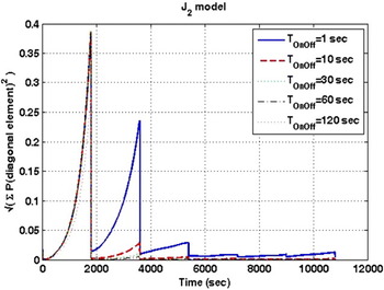
Figure 11. Variation of covariance matrices calculated using different GPS receiver On/Off time intervals.

Figure 12. X Y and Z position error in ODS with J2 model, Tact=1800 sec and TOn/Off=60 sec.
6.2. Performance Evaluation of Fault Management System
In this scenario, performance of the proposed fault management system is investigated. For this purpose, different bias and ramp type faults have been included in this section. Note that most faults which occur in the GPS are of bias or ramp type (Joerger Reference Joerger, Neale and Pervan2009; Bruggemann Reference Bruggemann, Greer and Walker2011). As shown in Figure 13 (a), a bias fault f equal to 50% of the maximum value that provided by the GPS in healthy condition, is introduced at time t=5000s in all three components of GPS1. Since this GPS is turned on every 30 min with a duration of 60 s (Figure 13 (a)), the mentioned fault is first detected at time t=5400s. Figure 14 shows that the norm error that prior to fault occurrence is less that 1 km, suddenly exceeds the threshold value. For this, the value 500 km has been selected for the threshold value. Also, after fault occurence, the components values x, y and z estimated by the EKF (Figure 15) have experienced sudden deviations.

Figure 13. Time line of GPS receivers activity (a) fault occurrence in GPS1 (b) fault occurrence in GPS2 (c) activating the SGP4 algorithm after fault happening in GPS2.

Figure 14. (a) Norm error of GPS receivers during fault occurrence (b) the magnified norm error for GPS receivers.

Figure 15. Estimation components x, y and z generated by the EKF during fault occurrence in GPS receivers.
To make sure that the residuals have not changed due to noise or other transient effects, fault declaration is done with 5 samples delay (Figure 13 (a)). Upon fault declaration, a command is sent by the fault accommodation system to turn off GPS1. At this moment, GPS2 is turned on and substituted instead of GPS1 (Figures 13 (b) and 16). Note that in Figure 16, only the x component of GPS receivers has been depicted. After replacement of GPS2, the residual (Figure 14 (b)) will return again below the selected threshold value, also this allows provision of precise satellite position data (after a transient condition due to GPS substitution and convergence of filter) with an accuracy better than 1 km (Figure 14 (a)). These transient states can also be observed in the estimated components x, y and z in Figure 15.

Figure 16. The on/off profiles of GPS receivers.
In this scenario, it is assumed that another fault (sudden loss of all GPS signals) has occurred in GPS2 at time t=14 000s. As shown in Figure 13 (b), this event is first detected at time t=14 400s and is declared after a 5 sample delay. At this time, the residual has experienced again a drastic deviation (Figure 14 (a)) and sudden changes occur in the estimation components x, y and z (Figure 15). After fault declaration in GPS2, the accommodation system is activated and a command is sent to the C&DH.
Through issuing this command, the orbit determination system is switched to the SGP4 algorithm (Figure 13 (c)). Figure 14 (a) shows that this algorithm can prevent the estimation error from becoming too divergent and maintain them in a suitable bound of 20 kilometres. Although this error is not ideal, it can somewhat meet the imaging and attitude control requirements. In these simulations, it is assumed that upon activating the SGP4 algorithm, the TLE data is received from the ground station. This data is needed only once to reach the suitable error bound for position components.
Figure 17 shows the residual generated due to a bias fault with the magnitude 10% of the maximum value that provided by the GPS at time t=5399 s. As revealed from this figure, by reducing the fault magnitude, the value of the generated residual has been decreased (compared to Figure 14). In this case, similar to the previous scenario, the fault is declared after 5 samples delay. Note that in case of very small faults, the detection time may be increased or even may not be detected by the fault management system. For instance, Figure 18 shows the residual generated due to a bias fault with the magnitude 5% of the maximum value that is provided by the GPS. As can be observed in this figure, the residual is less than the threshold value in four consecutive times that GPS1 is turned on (or in duration lower than 5 samples delay it comes back again below the threshold value). Ultimately, this fault is detected at time t=12600 s. At this time, GPS2 is switched on by the fault management system.

Figure 17. Norm error of GPS receiver due to a bias fault with the magnitude 10% of the maximum value that provided by the GPS.

Figure 18. (a) Norm error of GPS receiver due to a bias fault with the magnitude 5% of the maximum value that provided by the GPS (b) the magnified form of the first turning on/off of GPS1 (c) the magnified form of the fifth (the last) turning on/off of GPS1.
Figure 19 depicts a ramp type fault with the slope 10 which has occurred at time t=5399 in all components of GPS1. As shown in Figure 20, the generated residual exceeds the threshold value after about 35 seconds (however the fault is declared by the fault management system after 40 samples due to the consideration of 5 samples delay) and it is substituted by GPS2. Similar to the bias type faults, by reducing the slope values, the fault is declared after several times of turning on/off the GPS1. Table 3 summarizes the performance of the fault management system against different fault types. According to this table, bias faults with the magnitude lower than 5% cannot be detected (the minimum detectable fault).

Figure 19. ramp type fault applied in all components of GPS1.

Figure 20. Norm error of GPS receiver due to ramp type fault with the slope 10.
Table 3. Performance of fault management system against different fault types.

7. CONCLUSIONS
In this paper a developed orbit determination system (ODS) was proposed which provides precise position information to support satellite attitude manoeuvres and to allow onboard real-time geocoding of the collected image data. For this, the satellite orbital parameters were estimated using an Extended Kalman Filter (EKF) in which the measurement data generated by two different Global Positioning System (GPS) receivers were utilized. Also, an analytical fault management system was suggested to provide fault detection, isolation and accommodation features. Accordingly, after fault occurrence in the main GPS, the required command for turning on the redundant one is issued. Also, the Simplified General Perturbations model 4 (SGP4) algorithm is utilized as a support analytical redundancy tool in conditions where both GPS receivers have failed. The simulation results demonstrated the suggested algorithm's performance in providing precise satellite position data with accuracy better than 1 km within an interval of 30 min. So, the developed algorithms propose an ability to provide position data despite power limitations. Also, utilizing the SGP4 algorithm described, sufficient onboard orbit determination accuracy is maintained for attitude determination and imaging purposes. In this paper, the fault management system was evaluated against different bias and ramp type faults and it is shown that the developed orbit determination system is capable of detecting outlined faults (although these functions were performed with a delay in some cases). Moreover, the minimum detectable bias was derived in our investigations.


