


I. INTRODUCTION
Much of microstructure science is focused on two intimately related tasks: (i) predicting the properties of a given microstructure and (ii) designing a microstructure to achieve a desired property. Both of these endeavors are fundamentally rooted in the notion that material structure determines material performance. Mathematically this idea has been canonized in various structure-property relations (see, e.g., Refs. Reference Kalidindi, Fullwood, Adams, Schwartz, Kumar, Adams and Field1, Reference Fullwood, Kalidindi, Adams, Schwartz, Kumar, Adams and Field2 and references therein). However, within the meso-scale microstructure community, rigorous theoretical developments have been largely restricted to the forward problem of property prediction. Various predictive models of material performance have been formulated and have proven successful. Reference Szpunar and Ojanen3–Reference Hutchinson and Swift5 However, the inverse problem of microstructure design has often consisted of an empirical trial-and-error approach.
Over the last decade, theoretical tools have been developed that allow materials designers to explore the complete universe of physically realizable microstructures for a given material and identify those that meet various performance objectives/design constraints. Reference Adams, Henrie, Henrie, Lyon, Kalidindi and Garmestani6,Reference Adams, Kalidindi and Fullwood7 This design formalism is referred to as microstructure sensitive design for performance optimization (MSDPO). Whereas the materials designer formerly had a finite (and rather incomplete) catalogue of observed microstructures and forward models at his/her disposal, the advent of these new microstructure design tools has allowed for the consideration of material structure as a continuous design variable and the rigorous solution of complex inverse design problems. Reference Adams, Henrie, Henrie, Lyon, Kalidindi and Garmestani6,Reference Lyon and Adams8–Reference Fast, Knezevic and Kalidindi14 While this advancement can hardly be understated, the present microstructure design paradigm has been limited to materials properties for which defect insensitive models exist, such as elasticity, conductivity, thermal expansion, and initial yield. Reference Adams, Henrie, Henrie, Lyon, Kalidindi and Garmestani6,Reference Lyon and Adams8–Reference Fast, Knezevic and Kalidindi14 However, other properties of scientific and engineering interest such as fracture, corrosion, and electromigration, which depend upon the structure of the grain boundary network, lie outside of its scope.
The experimental development of grain boundary engineering (GBE) Reference Watanabe15 has demonstrated the possibility of controllably varying the structure of grain boundary networks in an effort to improve materials properties. Reference Lehockey, Palumbo, Brennenstuhl and Lin16–Reference Lehockey, Palumbo and Lin19 However, materials amenable to this thermomechanical processing strategy are mostly limited to those that readily form annealing twins and exhibit appreciable plasticity. Furthermore, even for this class of materials, successful processing recipes have been developed through empirical iteration. If theoretical tools for designing grain boundary networks and predicting their effective properties were available, the benefits of GBE could be extended to a much broader class of materials and the pace of materials discovery and synthesis could be accelerated.
In the present work we demonstrate the first application of the MSDPO methodology to a defect sensitive property: grain boundary network diffusivity. Using a previously developed relationship between crystallographic texture and grain boundary network structure, Reference Johnson and Schuh20,Reference Johnson and Schuh21 we develop the mathematical tools necessary for a texture mediated approach to grain boundary network design. This mathematical apparatus is exercised in the context of a relatively simple, but illustrative, materials design problem.
II. DESIGN PROBLEM
As a simple example of a multiobjective microstructure optimization problem involving grain boundary networks, consider microstructure sensitive design
Reference Adams, Henrie, Henrie, Lyon, Kalidindi and Garmestani6,Reference Adams, Kalidindi and Fullwood7
of metallic interconnects for flexible electronics. Chemistry and geometry will be held constant (see Fig. 1) and we will seek to optimize the microstructure of a polycrystalline sample to satisfy certain design constraints and objectives. To limit the scope of the problem, we focus on aluminum with a simplified polycrystalline microstructure composed of regular hexagonal grains, each having an $\langle 001\rangle$
axis parallel to the sample z-direction.
$\langle 001\rangle$
axis parallel to the sample z-direction.

FIG. 1. System geometry. Above, the microstructure and loading conditions of a section of the Al interconnect is shown. A uniaxial stress, σ, is applied in the x-direction. An electrical current, J, also flows in the x-direction. The microstructure is composed of regular hexagonal grains all having their $\langle 001\rangle$
axis parallel to the sample z-direction. Below is a close-up of the region indicated by the red dashed circle. A triple junction is coordinated by grains with orientations ω1, ω2, and ω3, defined as the positive clockwise rotations from the sample x-direction. The grain boundary misorientations, ω12, ω23, and ω31 are also indicated.
$\langle 001\rangle$
axis parallel to the sample z-direction. Below is a close-up of the region indicated by the red dashed circle. A triple junction is coordinated by grains with orientations ω1, ω2, and ω3, defined as the positive clockwise rotations from the sample x-direction. The grain boundary misorientations, ω12, ω23, and ω31 are also indicated.
The design objectives for this study are summarized below:
 $${\bf max}\,\overline {{\sigma _{y1}}}$$
 $$\overline {{S_{1111}}} = S_{1111}^{{\rm{sub}}}$$
 $${\bf min} \,\overline D$$
In Eq. (1a), $\overline {{\sigma _{y1}}}$
represents the effective macroscopic yield strength in the x-direction (loading direction), which is an important consideration in this flexible electronics application both for static loading and because it correlates with fatigue strength.
Reference Suresh22,Reference Webster and Bannister23
In Eq. (1b) we require that the effective elastic constant,
$\overline {{\sigma _{y1}}}$
represents the effective macroscopic yield strength in the x-direction (loading direction), which is an important consideration in this flexible electronics application both for static loading and because it correlates with fatigue strength.
Reference Suresh22,Reference Webster and Bannister23
In Eq. (1b) we require that the effective elastic constant, $\overline {{S_{1111}}}$
, match that of the substrate,
$\overline {{S_{1111}}}$
, match that of the substrate, $S_{1111}^{{\rm{sub}}}$
, to which it is applied. Finally, in Eq. (1c) we seek to minimize the effective diffusivity of the grain boundary network,
$S_{1111}^{{\rm{sub}}}$
, to which it is applied. Finally, in Eq. (1c) we seek to minimize the effective diffusivity of the grain boundary network, $\overline D$
, to mitigate degradation due to electromigration.
$\overline D$
, to mitigate degradation due to electromigration.
The design variables for this case study include crystallographic texture and the crystallographic structure of the grain boundary network. We seek a distribution of crystal orientations and commensurate grain boundary network that will optimally satisfy the design constraints and performance objectives listed in Eq. (1).
III. QUANTIFYING MICROSTRUCTURE
The texture of a polycrystal may be described quantitatively by its orientation distribution function (ODF), denoted f(ω), where the quantity f(ω)dω indicates the probability of observing a grain whose orientation is infinitesimally close to ω. An ODF can be expanded as a harmonic series Reference Adams, Henrie, Henrie, Lyon, Kalidindi and Garmestani6,Reference Adams, Kalidindi and Fullwood7,Reference Johnson and Schuh20,Reference Johnson and Schuh21,Reference Bunge24 and, in the present case, may be expressed as:
 $$f\left( \omega \right) = \sum\limits_{k = - \infty }^\infty {{c_k}{{{\rm e}^{ik\omega }}} \quad ,$$
which is the familiar complex Fourier series. We take the convention that f(ω) is normalized over the entirety of S 1, which implies that c 0 = (2π)−1. Also, letting s denote the order of the cyclic rotational symmetry of the crystal system (s = 4 for the specific case under consideration), we have that c ns = 0 ∀ n ∉ ℤ. An alternative series expansion can be obtained in the basis of Dirac delta functions, according to:
 $$f\left( \omega \right) \approx \sum\limits_{l = 1}^L {{p_l}{\rm{\delta }}\left( {{\rm{\omega }} - {}^l{\rm{\omega }}} \right)} \quad ,$$
where each of the basis functions is centered at one of a discrete set of fundamental orientations, {1ω, 2ω, … , L ω}, which will be described later. The approximation in Eq. (3) becomes exact as L → ∞. We will use both the Fourier and the Dirac representations and, consequently, it will be necessary to translate between the two. By taking the Fourier transform of Eq. (3), we obtain the desired relationship:
 $${c_k} \approx \sum\limits_{l = 1}^L {{p_l}\,{}^l{c_k}} \quad ,$$
where l c k is the k-th coefficient of a microstructure composed entirely of the l-th fundamental orientation (i.e., a single crystal with orientation l ω).
The crystallographic structure of the grain boundary network can be quantified via the triple junction distribution function (TJDF), Reference Johnson and Schuh20,Reference Johnson and Schuh21,Reference Mason and Schuh25 denoted T(ω12, ω23), where the quantity T(ω12, ω23)dω12dω23 provides the probability of observing a triple junction in the microstructure that is coordinated by an ordered pair of grain boundary misorientations infinitesimally close to (ω12, ω23) (see also Refs. Reference Hardy and Field26 and Reference Hardy and Field27, which describe a related function). We define the misorientation between adjacent grains A and B by ωAB = ωB − ωA. Because of conservation of misorientation around a circuit enclosing a triple junction Reference Bollmann28 we have ω12 + ω23 + ω31 = 0, indicating that only two of the three possible misorientations are independent. As a convention we take the first two grain boundary misorientations, (ω12, ω23), as the independent ones that characterize a given triple junction. Like the ODF, the TJDF can be expressed in spectral form, Reference Johnson and Schuh20,Reference Johnson and Schuh21 and in the present two-dimensional case, may be represented in the basis of bipolar complex exponentials:
 $$T\left( {{\omega _{12}},{\omega _{23}}} \right) = \sum\limits_{{k_1},{k_3}} {\mathop {{t_{{k_1}}^{{k_3}} {{\rm e}^{i{k_1}{\omega _{12}}}}{{\rm e}^{i{k_3}{\omega _{23}}}}} \quad ,$$
where the indices k 1, k 3 ∈ (−∞, ∞), and the coefficients are determined using Eq. (A1). Other relevant properties of the TJDF and its coefficients are given in Appendix A, including constraints on the TJDF coefficients resulting from crystallographic and triple junction symmetries. The TJDF also admits a Dirac basis representation:
 $$T\left( {\omega _{12} ,\omega _{23} } \right) = \sum\limits_{n = 1}^N {\phi _n \delta \left[ {\left( {\omega _{12} ,\omega _{23} } \right),\left( {{}^n\omega _{12} ,{}^n\omega _{23} } \right)} \right]} \quad ,$$
where δ[(ω12, ω23), ( n ω12, n ω23)] ≡ δ(ω12 − n ω12) δ(ω23 − n ω23) so that the basis functions are centered at fundamental triple junctions (as characterized by the corresponding ordered pair of triple junction misorientations).
IV. MICROSTRUCTURE SETS AND HULLS
The spectral coefficients of an ODF, {… , c −1, c 0, c 1, …}, encode the texture of a given polycrystalline microstructure. These coefficients can be interpreted as the coordinates of a point in Fourier space that represents that texture (see Fig. 2). Microstructures with different textures will have different coefficients, corresponding to points with different coordinates. By considering all possible simultaneous values that the coefficients can take, one can define a region in Fourier space containing all physically possible textures. This region is called the texture hull. This formalism can be extended to bound the space of grain boundary networks using the spectral coefficients of the TJDF, in which case we obtain a triple junction hull. Such closed convex regions are generically referred to as microstructure hulls and the solution of our design problem involves searching the appropriate microstructure hull for a microstructure whose properties optimally satisfy our design objectives. In this section we explain the process of generating the relevant microstructure hulls.

FIG. 2. Schematic illustration of the texture hull in the Fourier basis. Points, with coordinates (c 1, c 2), correspond to textures as indicated by the selected inverse pole figures. The grey region bounding all of the points represents the texture hull, which is closed and convex. As the number of coefficients is infinite, this space is infinite dimensional. It is shown here as an orthogonal projection in two-dimensions.
A. The fundamental zone
In the two-dimensional case considered here, grain orientations take values ω ∈ [0, 2π), which may be interpreted as points on the unit circle, S 1. Due to crystallographic symmetry, the range of physically distinct orientations is restricted to ω ∈ [0, ω s ), where ω s ≡ 2π/s. This sub-space of S 1, is referred to as the fundamental zone or asymmetric region for grain orientations, and we denote it by:
 $${{\cal A}^{\left( 1 \right)}} = \left\{ {\omega\, \left|\, {\omega \in [0,{\omega _s}),\,\, {\omega _s} \equiv {{2\pi } \over s}} \right.} \right\}\quad .$$
In similar fashion, grain boundary misorientations, ωAB ≡ ω B − ω A, live on S 1, and, consequently, an ordered pair of independent triple junction misorientations, (ω12, ω23), inhabits the product space S 1 × S 1. The application of crystal symmetry operations to the orientations of any of the three grains coordinating a triple junction will leave the triple junction physically unchanged. Consequently we have that
 $$\left( {\omega _{12} ,\omega _{23} } \right) \,\sim\, \left( {\omega _{12} + a\omega _s ,\omega _{23} + b\omega _s } \right)\,\forall \,a,b \in ℤ$$
(see Appendix A.3 for a derivation). Furthermore, there are $\left( {\matrix{ 3 \cr 2 \cr } } \right)$
ways of selecting the 2 independent misorientations characterizing the triple junction, resulting in the following set of equivalence relations (see Ref. Reference Johnson and Schuh20):
$\left( {\matrix{ 3 \cr 2 \cr } } \right)$
ways of selecting the 2 independent misorientations characterizing the triple junction, resulting in the following set of equivalence relations (see Ref. Reference Johnson and Schuh20):
 $$\left( {{\omega _{12}},{\omega _{23}}} \right)\, \sim\, \left( {{\omega _{12}},{\omega _{23}}} \right)$$
 $$\left( {{\omega _{12}},{\omega _{23}}} \right)\, \sim\, \left( {{\omega _{23}}, - {\omega _{12}} - {\omega _{23}}} \right)$$
 $$\left( {{\omega _{12}},{\omega _{23}}} \right)\, \sim\, \left( { - {\omega _{12}} - {\omega _{23}},{\omega _{12}}} \right)$$
 $$\left( {{\omega _{12}},{\omega _{23}}} \right)\, \sim\, \left( { - {\omega _{12}},{\omega _{12}} + {\omega _{23}}} \right)$$
 $$\left( {{\omega _{12}},{\omega _{23}}} \right)\, \sim\, \left( {{\omega _{12}} + {\omega _{23}}, - {\omega _{23}}} \right)$$
 $$\left( {{\omega _{12}},{\omega _{23}}} \right)\, \sim\, \left( { - {\omega _{23}}, - {\omega _{12}}} \right)$$
which define the physical symmetries of triple junctions in the present two-dimensional case. Considering both crystal symmetry and triple junction symmetry, we can define a canonical fundamental zone for triple junction misorientations according to:
 $${\cal A}^{\left( 3 \right)} = \left\{ {\left( {\omega _{12} ,\omega _{23} } \right) {\,\left|\,\, {\omega _{23} \, \ge \,0,\omega _{23} \, \le \,\omega _{12} ,\omega _{23} \, \lt \,{1 \over 2}} \right.\left( {\omega _s - \omega _{12} } \right)} \right} \right\}\quad ,$$
which is illustrated graphically in Fig. 3, along with the symmetrically equivalent portions of the triple junction space. We note that a similar result was previously obtained by Mason in Ref. Reference Mason and Schuh25. The TJDF must repeat itself over each of the regions symmetrically equivalent to ${{\cal A}^{\left( 3 \right)}}$
. This requirement results in certain relationships among the TJDF coefficients (given in Appendix A), which limit the number of independent coefficients that need to be computed.
${{\cal A}^{\left( 3 \right)}}$
. This requirement results in certain relationships among the TJDF coefficients (given in Appendix A), which limit the number of independent coefficients that need to be computed.

FIG. 3. The fundamental zone for triple junction misorientations, ${{\cal A}^{\left( 3 \right)}}$
, shown in red. The other triangular regions in the detail view are symmetrically equivalent to the canonical
${{\cal A}^{\left( 3 \right)}}$
, shown in red. The other triangular regions in the detail view are symmetrically equivalent to the canonical ${{\cal A}^{\left( 3 \right)}}$
and are related by triple junction symmetries [Eq. (9)]. Crystallographic symmetries [Eq. (8)] cause the region shown in the detail view to be repeated throughout the remainder of S
1 × S
1.
${{\cal A}^{\left( 3 \right)}}$
and are related by triple junction symmetries [Eq. (9)]. Crystallographic symmetries [Eq. (8)] cause the region shown in the detail view to be repeated throughout the remainder of S
1 × S
1.
B. The microstructure set
By discretizing the fundamental zones ( ${{\cal A}^{\left( 1 \right)}}$
and
${{\cal A}^{\left( 1 \right)}}$
and ${{\cal A}^{\left( 3 \right)}}$
) we obtain sets of fundamental orientations and fundamental triple junctions, respectively, on which the Dirac basis functions of Eqs. (3) and (6) are centered. Consider a single crystal with orientation
l
ω. The coefficients of its ODF, in the Dirac representation, are all zero except for the l-th coefficient, which is equal to unity. We can represent this set of coefficients as a vector,
l
p
, whose l-th element is equal to 1 and all others are 0. The L coefficient vectors corresponding to the fundamental orientations form a microstructural basis in which an arbitrary ODF can be expressed. This is referred to as the texture set and it is defined by
${{\cal A}^{\left( 3 \right)}}$
) we obtain sets of fundamental orientations and fundamental triple junctions, respectively, on which the Dirac basis functions of Eqs. (3) and (6) are centered. Consider a single crystal with orientation
l
ω. The coefficients of its ODF, in the Dirac representation, are all zero except for the l-th coefficient, which is equal to unity. We can represent this set of coefficients as a vector,
l
p
, whose l-th element is equal to 1 and all others are 0. The L coefficient vectors corresponding to the fundamental orientations form a microstructural basis in which an arbitrary ODF can be expressed. This is referred to as the texture set and it is defined by
 $$M_{\rm{S}}^{\left( 1 \right)} = \left\{ {{^l{\bi p}\,\left|\, {{}^l{\bi p} = \left( {{}^l{p_{\rm{1}}},{}^l{p_{\rm{2}}}, \ldots ,{}^l{p_L}} \right),\,\,{}^l{p_r} = {{\rm{\delta }}_{rl}},\,\,l \in \left[ {1,L} \right]} \right.} \right\}\quad .$$
In light of the relationship between the Fourier and Dirac representations embodied in Eq. (4), the texture set can also be expressed in the Fourier representation:
 $$m_{\rm{S}}^{\left( 1 \right)} = \left\{ {{}^l{\bi c}\,\left|\, {{}^l{\bi c} = \left( { \ldots ,{}^lc_{ - {\rm{1}}} ,{}^lc_0 ,{}^lc_1 , \ldots } \right),{}^lc_k = {1 \over {2\pi }}{\rm e}^{ - ik{}^l{\rm{\omega }}} ,\,{}^l{\rm{\omega }} \in {\cal A}^{\left( 1 \right)} ,} \right.\,l \in \left[ {1,L} \right],\,k \in \left( { - \infty ,\infty } \right)} \right\}$$
and both representations will be used in the present work. To make our notation explicit, we will use capital letters when referring to the Dirac basis $\hbox( {M_{\rm{S}}^{\left( 1 \right)}} \hbox)$
, lower-case letters when referring to the Fourier basis
$\hbox( {M_{\rm{S}}^{\left( 1 \right)}} \hbox)$
, lower-case letters when referring to the Fourier basis $\hbox( {m_{\rm{S}}^{\left( 1 \right)}} \hbox)$
, and calligraphic script when referring to the abstract concept independent of either representation (e.g.,
$\hbox( {m_{\rm{S}}^{\left( 1 \right)}} \hbox)$
, and calligraphic script when referring to the abstract concept independent of either representation (e.g., ${\cal M}_{\rm{S}}^{\left( 1 \right)}$
). Bold face is used to indicate a vector quantity.
${\cal M}_{\rm{S}}^{\left( 1 \right)}$
). Bold face is used to indicate a vector quantity.
In like fashion to the texture set, a triple junction set is defined by
 $$M_{\rm{S}}^{\left( 3 \right)} = \left\{ {{}^n\boldphi\, |\,{}^n\boldphi = \left( {{}^n{\phi _1},{}^n{\phi _2}, \ldots ,{}^n{\phi _{N}}} \right),\,\,{}^n{\phi _r} = {\delta _{rn}},\,\,n \in \left[ {1,N} \right]} \right\}$$
or
 $$m_{\rm{S}}^{\left( 3 \right)} = \left\{ {{}^n{\bi t}\,\left|\, {{}^n{\bi t} = \left( { \ldots ,{}^nt_{ - {\rm{1}}}^0,{}^nt_{ - {\rm{1}}}^1, \ldots ,{}^nt_{\rm{0}}^0,{}^nt_{\rm{0}}^1, \ldots } \right)} \right.,{}^n\mathop {{t_{{k_{\rm{1}}}}^{{k_3}} = {1 \over {4{\pi ^2}}}{\rm e}^{ - i{k_1}{}^n{\omega _{12}}}}{\rm e}^{ - i{k_3}{}^n{\omega _{23}}}},\,\,\left( {{}^n{\omega _{12}},{}^n{\omega _{23}}} \right) \in {{\cal A}^{\left( 3 \right)}},\,\,n \in \left[ {1,N} \right],\,\,{k_1},{k_3} \in \left( { - \infty ,\infty } \right)} \right\}\quad .$$
The importance of these microstructure sets stems from the fact that they are fundamental building blocks from which a statistical description (i.e., the ODF or TJDF) of any microstructure can be constructed. This can be seen from the form of Eq. (4), in which the Fourier coefficients of an arbitrary ODF can be expressed as a weighted sum of the elements of $m_{\rm{S}}^{\left( 1 \right)}$
with the Dirac coefficients providing the weights. A similar expression exists in the case of the TJDF coefficients:
$m_{\rm{S}}^{\left( 1 \right)}$
with the Dirac coefficients providing the weights. A similar expression exists in the case of the TJDF coefficients:
 $$\mathop {{t_{{k_1}}^{{k_3}} \approx \sum\limits_{n = 1}^N {{\phi _n}\,{}^n\mathop {{t_{{k_1}}^{{k_3}} } \quad .$$
For the case study considered here, we use a resolution of 5° for both $M_{\rm{S}}^{\left( 1 \right)}$
and
$M_{\rm{S}}^{\left( 1 \right)}$
and $M_{\rm{S}}^{\left( 3 \right)}$
.
$M_{\rm{S}}^{\left( 3 \right)}$
.
C. The microstructure hull
The goal of the design problem considered here is to identify a microstructure whose properties will optimally satisfy the design objectives expressed in Eq. (1). As will be explained in Sec. V, the constitutive models that we use consider the influence of both texture and grain boundary network structure. Thus, the design space for this problem comprises the space of all possible ODFs and all possible TJDFs. One of the advantages of the spectral form for ODFs and TJDFs given in Sec. III is that it facilitates a concrete mathematical description of this design space. By enumerating all physically possible simultaneous values of the ODF coefficients, {c
k
} or {p
l
}, we can consider all possible textures and this defines the design space for textures. The same can be done with the TJDF coefficients to define the design space for grain boundary networks. This can be accomplished most easily in the Dirac basis. Because the ODF is a probability density function, we have a normalization condition, $\int_0^{2{\rm{\pi }}} {f\left( {\rm{\omega }} \right) = 1}$
, and a requirement of non-negativity, f(ω) ≥ 0. The normalization condition implies that
$\int_0^{2{\rm{\pi }}} {f\left( {\rm{\omega }} \right) = 1}$
, and a requirement of non-negativity, f(ω) ≥ 0. The normalization condition implies that $\sum\limits_{l = 1}^L {{p_l}} = 1$
and the non-negativity requirement guarantees that p
l
≥ 0 ∀ l. These conditions mean that in the Dirac basis, the space of all possible ODFs is an (L − 1)-dimensional simplex: the convex hull of the texture set,
$\sum\limits_{l = 1}^L {{p_l}} = 1$
and the non-negativity requirement guarantees that p
l
≥ 0 ∀ l. These conditions mean that in the Dirac basis, the space of all possible ODFs is an (L − 1)-dimensional simplex: the convex hull of the texture set, $M_{\rm{S}}^{\left( 1 \right)}$
, the elements of which form the vertices. We therefore refer to this space as the texture hull. Its formal definition may be expressed as
$M_{\rm{S}}^{\left( 1 \right)}$
, the elements of which form the vertices. We therefore refer to this space as the texture hull. Its formal definition may be expressed as
 $$M_{\rm{H}}^{\left( 1 \right)} = \left\{ {{\bi p}\,\left|\, \,{{\bi p} = \left( {{p_1},{p_2}, \ldots ,{p_L}} \right),\,\,0 \,\le\, {p_l}\,\forall\, l,\sum\limits_{l = 1}^L {{p_l}} = 1} \right.} \right\}\quad .$$
Using Eq. (4), the texture hull can be expressed in the Fourier basis as well according to
 $$m_{\rm{H}}^{\left( 1 \right)} = \left\{ {{\bi c}\,\left|\, {{\bi c}\, \approx \,\mathop {\sum \limits_{l = 1}^L p_l\, {}_{}^l {\bi c},\;{}_{}^l {\bi c} \in m_{\rm{S}}^{\left( 1 \right)} ,\,\,0 \,\le\, p_l \,\forall\,\, l,\;\sum\limits_{l = 1}^L {p_l } = 1} \right} \right\}\quad .$$
The same process yields the design space for grain boundary networks, the triple junction hull:
 $$M_{\rm{H}}^{\left( 3 \right)} = \left\{ {\boldphi \,\left|\, {\boldphi = \left( {{\phi _1},{\phi _2}, \ldots ,{\phi _N}} \right),\,\,0 \,\le\, {\phi _n}\,\forall\, n,\sum\limits_{n = 1}^N {{\phi _n}} = 1} \right.} \right\}$$
in the Dirac representation, or
 $$m_{\rm{H}}^{\left( 3 \right)} = \left\{ {{\bi t}\,\left|\, {{\bi t}\, \approx \,\mathop {\sum \limits_{n = 1}^N \phi _n\, {}^n{\bi t},\,{}^n{\bi t}\, \in \,m_{\rm{S}}^{\left( 3 \right)} ,\,0\, \le \,\phi _n \,\,\forall \,\,n,\,\sum\limits_{n = 1}^N {\phi _n = 1} } \right} \right\}$$
in the Fourier representation.
It is important to note that texture and grain boundary network structure are not independent microstructural features, but neither does one fully specify the other. To find a physically valid solution to our design problem we cannot search ${\cal M}_{\rm{H}}^{\left( 1 \right)}$
and
${\cal M}_{\rm{H}}^{\left( 1 \right)}$
and ${\cal M}_{\rm{H}}^{\left( 3 \right)}$
independently, but, rather, we must find an optimal texture and grain boundary network that are self-consistent (i.e., compatible). To accomplish this we will consider the subset of microstructures for which spatial correlations in grain orientation are absent. For this reduced set of microstructures each texture (ODF) associates with exactly one grain boundary network (TJDF). This mapping has been published previously for the full 3D case
Reference Johnson and Schuh20,Reference Johnson and Schuh21
; here, we provide the formula for the 2D case relevant to the present design problem:
${\cal M}_{\rm{H}}^{\left( 3 \right)}$
independently, but, rather, we must find an optimal texture and grain boundary network that are self-consistent (i.e., compatible). To accomplish this we will consider the subset of microstructures for which spatial correlations in grain orientation are absent. For this reduced set of microstructures each texture (ODF) associates with exactly one grain boundary network (TJDF). This mapping has been published previously for the full 3D case
Reference Johnson and Schuh20,Reference Johnson and Schuh21
; here, we provide the formula for the 2D case relevant to the present design problem:
 $$\mathop {{{\tilde t}_{{k_1}}^{{k_3}} = 2{\rm{\pi }}c_{{k_1}}^*{c_{{k_1} - {k_3}}}{c_{{k_3}}}\quad .$$
This expression permits the computation of the TJDF coefficients of a microstructure from a knowledge of its ODF coefficients. We include the tilde to indicate that these are the uncorrelated TJDF coefficients, or the TJDF coefficients computed under the assumption that the grain orientations are spatially uncorrelated (see Appendix B). Equation (20) allows us to define an uncorrelated triple junction hull:
 $$\tilde m_{\rm{H}}^{\left( 3 \right)} = \left\{ {\tilde {\bi t}\,|\,\tilde {\bi t}\, \equiv \,\left\{ {\mathop {\tilde t_{k_1 } ^{k_3 } }} \right\},\,\mathop {\tilde t_{k_1 }^{k_3 } = 2{\rm{\pi }}c_{k_1 }^{\rm{*}} c_{k_1 - k_3 } c_{k_3 } ,\,{\bi c}\, \equiv \,\left\{ {c_k } \right\},\,{\bi c} \in m_{\rm{H}}^{\left( 1 \right)} }} \right\}\quad .$$
Each point in ${\cal M}_{\rm{H}}^{\left( 1 \right)}$
maps to exactly one point in
${\cal M}_{\rm{H}}^{\left( 1 \right)}$
maps to exactly one point in $\widetilde {\cal M}_{\rm{H}}^{\left( 3 \right)}$
allowing us to find a self-consistent solution to our design problem.
$\widetilde {\cal M}_{\rm{H}}^{\left( 3 \right)}$
allowing us to find a self-consistent solution to our design problem.
The mapping embodied in Eq. (20) is, however, many-to-one which can be seen in the inverse mapping (derived in Appendix B):
 $$<tex-math>{c_{\eta s}} = \left\{ {\matrix{ {{c_0}\prod\limits_{j = 1}^{{\eta \mathord{\left/ {\vphantom {\eta 2}} \right. \kern-\nulldelimiterspace} 2}} {{{\tilde t_s^{\left( {2j} \right)s}} \over {\tilde t_{\left( {2j - 1} \right)s}^s}}} } & {{\rm{for}}\;{\mathop{\rm even}\nolimits} \,\eta } \cr {{c_s}\prod\limits_{j = 1}^{{{\left( {\eta - 1} \right)} \mathord{\left/ {\vphantom {{\left( {\eta - 1} \right)} 2}} \right. \kern-\nulldelimiterspace} 2}} {{{\tilde t_s^{\left( {2j + 1} \right)s}} \over {\tilde t_{\left( {2j} \right)s}^s}}} } & {{\rm{for}}\;{\mathop{\rm odd}\nolimits} \,\eta } \cr} } \right.</tex-math>$$
where again s denotes the order of the cyclic rotational symmetry of the crystal system. All of the quantities on the right hand side of Eq. (22) are fully defined except for the phase of c
s
, which is a free parameter (see Appendix B). This indicates that it is possible to recover an ODF from a TJDF modulo a rotation operation (see Fig. 4). In other words, all ODFs that differ only by a rotation (e.g., f(ω) and f(ω + Δω)) correspond to the same TJDF. In light of this invertible relationship between ODF and TJDF, it is possible to obtain a microstructural solution with self-consistent ODF and TJDF via a texture-mediated approach, i.e. by adopting ${\cal M}_{\rm{H}}^{\left( 1 \right)}$
as our formal microstructural design space and mapping it to
${\cal M}_{\rm{H}}^{\left( 1 \right)}$
as our formal microstructural design space and mapping it to ${\cal M}_{\rm{H}}^{\left( 3 \right)}$
as necessary. The process used to accomplish this is described in Sec. VI(B).
${\cal M}_{\rm{H}}^{\left( 3 \right)}$
as necessary. The process used to accomplish this is described in Sec. VI(B).

V. CONSTITUTIVE MODELS
With a mathematical description of microstructure in hand, we are prepared to consider constitutive models for the materials properties relevant to our design problem. Microstructure sensitive models for $\overline {{S_{1111}}}$
and
$\overline {{S_{1111}}}$
and $\overline {{{\rm{\sigma }}_{y1}}}$
are readily available. Below, we explain the application of each of these properties models to the present design problem. We also develop a model for
$\overline {{{\rm{\sigma }}_{y1}}}$
are readily available. Below, we explain the application of each of these properties models to the present design problem. We also develop a model for $\bar D$
that depends on the types and populations of grain boundaries and triple junctions present in the polycrystal.
$\bar D$
that depends on the types and populations of grain boundaries and triple junctions present in the polycrystal.
A. Yield
The effective macroscopic yield strength of our polycrystalline material can be approximated using the model developed by Sachs, Reference Sachs29,Reference Wu, Proust, Knezevic and Kalidindi30 according to:
 $$\overline {{\sigma _{y1}}} = {{\rm{\tau }}_{{\rm{CRSS}}}}\overline {\left( {{1 \over{\displaystyle{\max\atop {\vskip-8pt\rm{\alpha }}}\vskip-4pt \left| {\mathop {{b_1}}\nolimits\!\!\!^{\rm{\alpha }} \left( q \right)\mathop {{n_1}}\nolimits\!\!\!^{\rm{\alpha }} \left( q \right)} \right|}}} \right)} \quad ,$$
where τCRSS is the critically resolved shear stress (0.79 MPa for Al
Reference Tiryakioglu, Staley, Totten and Mackenzie31
), $\mathop {{b_1}}\nolimits\!\!\!^{\rm{\alpha }} \left( q \right)$
and
$\mathop {{b_1}}\nolimits\!\!\!^{\rm{\alpha }} \left( q \right)$
and $\mathop {{n_1}}\nolimits\!\!\!^{\rm{\alpha }} \left( q \right)$
are the x-components of the slip direction and slip plane normal, respectively, of the α-th slip system–both of which are functions of the crystallographic orientation, q, in a given grain. The overbar indicates a volume average over all crystal orientations in the polycrystal. As mentioned in Sec. II, we will make the additional assumption that all orientations in our polycrystal share a common rotation axis that is orthogonal to the plane of the sample and which is a four-fold symmetry axis of the crystal (i.e., a
$\mathop {{n_1}}\nolimits\!\!\!^{\rm{\alpha }} \left( q \right)$
are the x-components of the slip direction and slip plane normal, respectively, of the α-th slip system–both of which are functions of the crystallographic orientation, q, in a given grain. The overbar indicates a volume average over all crystal orientations in the polycrystal. As mentioned in Sec. II, we will make the additional assumption that all orientations in our polycrystal share a common rotation axis that is orthogonal to the plane of the sample and which is a four-fold symmetry axis of the crystal (i.e., a $\langle 100\rangle$
direction for FCC aluminum as illustrated in Fig. 1). This makes the problem effectively two-dimensional and simplifies Eq. (23) to:
$\langle 100\rangle$
direction for FCC aluminum as illustrated in Fig. 1). This makes the problem effectively two-dimensional and simplifies Eq. (23) to:
 $$\overline {{{\rm{\sigma }}_{y1}}} = {{\rm{\tau }}_{{\rm{CRSS}}}}\int_0^{2{\rm{\pi }}} {f\left( {\rm{\omega }} \right)g\left( {\rm{\omega }} \right){\rm{d\omega }}} \quad ,$$
where the scalar ω is an orientation, f(ω) is an ODF, and g(ω) is defined by:
 $$g\left( \omega \right) = \left\{ {\matrix{ {{{\left[ {{{{\rm{cos}}\,\omega \,\left( {{\rm{sin}}\,\omega + {\rm{cos}}\,\,\omega } \right)} \mathord{\left/ {\vphantom {{{\rm{cos}}\,\omega \left( {{\rm{sin}}\,\omega + {\rm{cos}}\,\,\omega } \right)} {\sqrt 6 }}} \right. \kern-\nulldelimiterspace} {\sqrt 6 }}} \right]}^{ - 1}}} & {{\rm{for}}\;\omega \in \left[ {0,{{\rm{\pi }} \mathord{\left/ {\vphantom {{\rm{\pi }} 4}} \right. \kern-\nulldelimiterspace} 4}} \right],\left[ {{\rm{\pi }},{{5{\rm{\pi }}} \mathord{\left/ {\vphantom {{5{\rm{\pi }}} 4}} \right. \kern-\nulldelimiterspace} 4}} \right]} \cr {{{\left[ {{{{\rm{sin}}\,\omega \,\left( {{\rm{sin}}\,\omega + {\rm{cos}}\,\omega } \right)} \mathord{\left/ {\vphantom {{{\rm{sin}}\,\omega \left( {{\rm{sin}}\,\omega + {\rm{cos}}\,\omega } \right)} {\sqrt 6 }}} \right. \kern-\nulldelimiterspace} {\sqrt 6 }}} \right]}^{ - 1}}} & {{\rm{for}}\;\omega \in \left[ {{{\rm{\pi }} \mathord{\left/ {\vphantom {{\rm{\pi }} 4}} \right. \kern-\nulldelimiterspace} 4},{{\rm{\pi }} \mathord{\left/ {\vphantom {{\rm{\pi }} {\rm{2}}}} \right. \kern-\nulldelimiterspace} {\rm{2}}}} \right],\left[ {{{5{\rm{\pi }}} \mathord{\left/ {\vphantom {{5{\rm{\pi }}} 4}} \right. \kern-\nulldelimiterspace} 4},{{6{\rm{\pi }}} \mathord{\left/ {\vphantom {{6{\rm{\pi }}} 4}} \right. \kern-\nulldelimiterspace} 4}} \right]} \cr {{{\left[ {{{{\rm{sin}}\,\omega \,\left( {{\rm{sin}}\,\omega - {\rm{cos}}\,\,\omega } \right)} \mathord{\left/ {\vphantom {{{\rm{sin}}\,\omega \left( {{\rm{sin}}\,\omega - {\rm{cos}}\,\,\omega } \right)} {\sqrt 6 }}} \right. \kern-\nulldelimiterspace} {\sqrt 6 }}} \right]}^{ - 1}}} & {{\rm{for}}\;\omega \in \left[ {{{\rm{\pi }} \mathord{\left/ {\vphantom {{\rm{\pi }} {\rm{2}}}} \right. \kern-\nulldelimiterspace} {\rm{2}}},{{3{\rm{\pi }}} \mathord{\left/ {\vphantom {{3{\rm{\pi }}} 4}} \right. \kern-\nulldelimiterspace} 4}} \right],\left[ {{{6{\rm{\pi }}} \mathord{\left/ {\vphantom {{6{\rm{\pi }}} 4}} \right. \kern-\nulldelimiterspace} 4},{{7{\rm{\pi }}} \mathord{\left/ {\vphantom {{7{\rm{\pi }}} 4}} \right. \kern-\nulldelimiterspace} 4}} \right]} \cr {{{\left[ {{{ - {\rm{cos}}\,\omega \,\left( {{\rm{sin}}\,\omega - {\rm{cos}}\,\,\omega } \right)} \mathord{\left/ {\vphantom {{ - {\rm{cos}}\,\omega \left( {{\rm{sin}}\,\omega - {\rm{cos}}\,\,\omega } \right)} {\sqrt 6 }}} \right. \kern-\nulldelimiterspace} {\sqrt 6 }}} \right]}^{ - 1}}} & {{\rm{for}}\;\omega \in \left[ {{{3{\rm{\pi }}} \mathord{\left/ {\vphantom {{3{\rm{\pi }}} 4}} \right. \kern-\nulldelimiterspace} 4},{\rm{\pi }}} \right],\left[ {{{7{\rm{\pi }}} \mathord{\left/ {\vphantom {{7{\rm{\pi }}} 4}} \right. \kern-\nulldelimiterspace} 4},2{\rm{\pi }}} \right]} \cr} } \right.$$
The function g(ω) can also be represented in spectral form as
 $$g\left( {\rm{\omega }} \right) = \sum\limits_{k = - \infty }^\infty {g_k {\rm{e}}^{ik{\rm{\omega }}} } \quad .$$
Substituting Eqs. (2) and (26) into Eq. (24) and evaluating the integral yields
 $$\overline {{\rm{\sigma }}_{y1} } = 2{\rm{\pi \tau }}_{{\rm{CRSS}}} \,\sum\limits_{k = - \infty }^\infty {c_k^{\rm{*}} g_k } \quad ,$$
where we have made use of the reality condition, f(ω) = f*(ω), and the orthogonality of the Fourier basis functions. As has been pointed out by the MSDPO community in other contexts,
Reference Fullwood, Niezgoda, Adams and Kalidindi32
the form of Eq. (27) is significant in that it represents a decoupling of the microstructural information (encoded in c
k
) from the physics of the material phenomena (encoded in g
k
). The properties coefficients, g
k
, need only be computed once, and then $\overline {{{\rm{\sigma }}_{y1}}}$
may be easily and efficiently evaluated for any microstructure through the inner product operation represented by Eq. (27), which is the two-dimensional analog of a result given previously in Ref. Reference Wu, Proust, Knezevic and Kalidindi30.
$\overline {{{\rm{\sigma }}_{y1}}}$
may be easily and efficiently evaluated for any microstructure through the inner product operation represented by Eq. (27), which is the two-dimensional analog of a result given previously in Ref. Reference Wu, Proust, Knezevic and Kalidindi30.
B. Elastic compliance
The Voigt model Reference Bunge24,Reference Voigt33 for elastic compliance assumes that all grains undergo the same elastic strain. This provides an upper bound, which, for the specific case at hand, can be expressed as:
 $$\overline {{S_{1111}}} = \int_0^{2{\rm{\pi }}} {f\left( {\rm{\omega }} \right){S_{1111}}\left( {\rm{\omega }} \right){\rm{d\omega }}}$$
with the orientation dependent function S 1111(ω) defined by:
 $${S_{1111}}\left( {\rm{\omega }} \right) = \,\,\left( {{\rm{co}}{{\rm{s}}^4}\,{\rm{\omega }} + {\rm{si}}{{\rm{n}}^4}\,{\rm{\omega }}} \right){S_{1111}} + 2\,{\rm{co}}{{\rm{s}}^2}\,{\rm{\omega }}\,{\rm{si}}{{\rm{n}}^2}\,{\rm{\omega }}\left( {{S_{1122}} + 2{S_{1212}}} \right)\quad .$$
Following the same procedure for elasticity as was employed above for yield, we may express Eq. (29) in spectral form:
 $$S_{1111} \left( {\rm{\omega }} \right) = \sum\limits_{k = - \infty }^\infty {s_k {\rm{e}}^{ik{\rm{\omega }}} }$$
with the elastic properties coefficients being given explicitly by
 $${s_k} = \left\{ {\matrix{ {{1 \over 8}\left[ {{S_{1111}} - \left( {{S_{1122}} + 2{S_{1212}}} \right)} \right]} & {k \in \left\{ { - 4,4} \right\}} \cr {{1 \over 4}\left[ {3{S_{1111}} + \left( {{S_{1122}} + 2{S_{1212}}} \right)} \right]} & {k = 0} \cr 0 & {{\rm{otherwise}}} \cr} } \right.$$
Substituting Eqs. (2) and (30) into Eq. (28) and evaluating the integral yields
 $$\overline {{S_{1111}}} = 2{\rm{\pi }}\sum\limits_{k \in \left\{ { - 4,0,4} \right\}} {c_k^{\rm{*}}{s_k}}$$
as an expression for the Voigt model of elastic compliance, expressed in spectral form.
C. Grain boundary network diffusivity
The diffusivities of individual grain boundaries can differ by orders of magnitude. This strong contrast of grain boundary diffusivity precludes the use of effective medium theory models to predict the effective diffusivity of grain boundary networks in polycrystals. Reference Reed, Schuh, Schwartz, Kumar, Adams and Field34 McLachlan proposed a phenomenological model for the effective electrical conductivity of binary mixtures of insulating and conducting phases, Reference McLachlan35,Reference McLachlan36 which was adapted to the analogous case of grain boundary network diffusivity by Chen and Schuh Reference Chen and Schuh37 :
 $${p_1}{{\mathop {{D_1}}\nolimits^{{1 \mathord{\left/ {\vphantom {1 s}} \right. \kern-\nulldelimiterspace} s}} - {{\left( {2\overline D} \right)}^{{1 \mathord{\left/ {\vphantom {1 s}} \right. \kern-\nulldelimiterspace} s}}}} \over {\mathop {{D_1}}\nolimits^{{1 \mathord{\left/ {\vphantom {1 s}} \right. \kern-\nulldelimiterspace} s}} + \left( {\mathop {{p_{c,2}}}\nolimits^{ - 1} - 1} \right){{\left( {2\overline D} \right)}^{{1 \mathord{\left/ {\vphantom {1 s}} \right. \kern-\nulldelimiterspace} s}}}}} + {p_2}{{\mathop {{D_2}}\nolimits^{{1 \mathord{\left/ {\vphantom {1 t}} \right. \kern-\nulldelimiterspace} t}} - {{\left( {2\overline D} \right)}^{{1 \mathord{\left/ {\vphantom {1 t}} \right. \kern-\nulldelimiterspace} t}}}} \over {\mathop {{D_2}}\nolimits^{{1 \mathord{\left/ {\vphantom {1 t}} \right. \kern-\nulldelimiterspace} t}} + \left( {\mathop {{p_{c,2}}}\nolimits^{ - 1} - 1} \right){{\left( {2\overline D} \right)}^{{1 \mathord{\left/ {\vphantom {1 t}} \right. \kern-\nulldelimiterspace} t}}}}} = 0\quad .$$
In this expression, p
1 and p
2 are the fraction of low- and high-angle grain boundaries, respectively, D
1 ≤ D
2 are the corresponding diffusivities, and $\bar D$
is the effective diffusivity of the grain boundary network (see Ref. Reference Johnson, Li, Demkowicz and Schuh38 for a discussion of the slight difference between the form of Eq. (33) and the corresponding equation provided in Ref. Reference Chen and Schuh37). The exponents are constants that depend only on the dimensionality of the problem and in this work are taken as s = 1.09 and t = 1.13. The spatial distribution of low- and high-angle grain boundaries in real materials is manifestly non-random and the percolation threshold for high-angle grain boundaries, p
c,2, is sensitive to these correlations in the grain boundary network,
Reference Schuh, Minich and Kumar39
which result from crystallographic constraints, texture, etc. These correlations are known to be short-range
Reference Frary and Schuh40
and can be quantified by the triple junction fractions, {J
i
| i ∈ [0, 3]}, which measure the fraction of triple junctions coordinated by i “special” grain boundaries (low-angle in the present context). Frary and Schuh found an empirical relation that predicts the percolation threshold (the expressions given in Ref. Reference Frary and Schuh41 were for p
c,1, but can be used to obtain p
c,2 by simply replacing Eq. (7b) of Ref. Reference Frary and Schuh41 with its reciprocal) as a function of the J
i,
Reference Frary and Schuh41
the details of which will be omitted here, but which allows us to write
$\bar D$
is the effective diffusivity of the grain boundary network (see Ref. Reference Johnson, Li, Demkowicz and Schuh38 for a discussion of the slight difference between the form of Eq. (33) and the corresponding equation provided in Ref. Reference Chen and Schuh37). The exponents are constants that depend only on the dimensionality of the problem and in this work are taken as s = 1.09 and t = 1.13. The spatial distribution of low- and high-angle grain boundaries in real materials is manifestly non-random and the percolation threshold for high-angle grain boundaries, p
c,2, is sensitive to these correlations in the grain boundary network,
Reference Schuh, Minich and Kumar39
which result from crystallographic constraints, texture, etc. These correlations are known to be short-range
Reference Frary and Schuh40
and can be quantified by the triple junction fractions, {J
i
| i ∈ [0, 3]}, which measure the fraction of triple junctions coordinated by i “special” grain boundaries (low-angle in the present context). Frary and Schuh found an empirical relation that predicts the percolation threshold (the expressions given in Ref. Reference Frary and Schuh41 were for p
c,1, but can be used to obtain p
c,2 by simply replacing Eq. (7b) of Ref. Reference Frary and Schuh41 with its reciprocal) as a function of the J
i,
Reference Frary and Schuh41
the details of which will be omitted here, but which allows us to write
 $${p_{c,2}} = {p_{c,2}}\left( {{J_0},{J_1},{J_2},{J_3}} \right)\quad .$$
The triple junction fractions can be interpreted as the average probability of observing a triple junction coordinated by i “special” grain boundaries in a given microstructure. Considering low-angle grain boundaries as “special”, this allows us to compute the J i by integration of the TJDF Reference Johnson and Schuh20,Reference Johnson and Schuh21 according to:
 $${J_i} = \int_{{{\rm{\Omega }}_i}} {T\left( {{{\rm{\omega }}_{12}},{{\rm{\omega }}_{23}}} \right){\rm{d}}{{\rm{\Omega }}_i}} \quad .$$
In Eq. (35), Ω i is the appropriate integration region as defined by:
 $${\rm{\Omega }}_0 = \left\{ {\left( {{\rm{\omega }}_{12} ,{\rm{\omega }}_{23} } \right)|{{\hat \omega }}_{12} \, > \,{\rm{\omega }}_t ,\,{{\hat \omega }}_{23} \, > \,{\rm{\omega }}_t ,\,{{\hat \omega }}_{31} \, > \,{\rm{\omega }}_t } \right\}$$
 $${\rm{\Omega }}_1 =\, \left\{ {\left( {{\rm{\omega }}_{12} ,{\rm{\omega }}_{23} } \right)|{{\hat \omega }}_{12} \, \le \,{\rm{\omega }}_t ,\,{{\hat \omega }}_{23} \, > \,{\rm{\omega }}_t ,\,{{\hat \omega }}_{31} \, > \,{\rm{\omega }}_t } \right\} \mathop {\cup} \nolimits\, \left\{ {\left( {{\rm{\omega }}_{12} ,{\rm{\omega }}_{23} } \right)|{{\hat \omega }}_{12} \, > \,{\rm{\omega }}_t ,\,{{\hat \omega }}_{23} \, \le \,{\rm{\omega }}_t ,\,{{\hat \omega }}_{31} \, > \,{\rm{\omega }}_t } \right\} \mathop {\cup} \nolimits\, \left\{ {\left( {{\rm{\omega }}_{12} ,{\rm{\omega }}_{23} } \right)|{{\hat \omega }}_{12} \, > \,{\rm{\omega }}_t ,\,{{\hat \omega }}_{23} \, > \,{\rm{\omega }}_t ,\,{{\hat \omega }}_{31} \, \le \,{\rm{\omega }}_t } \right\} \cr}$$
 $${\rm{\Omega }}_2 =\, \left\{ {\left( {{\rm{\omega }}_{12} ,{\rm{\omega }}_{23} } \right)|{{\hat \omega }}_{12} \, > \,{\rm{\omega }}_t ,\,{{\hat \omega }}_{23} \, \le \,{\rm{\omega }}_t ,\,{{\hat \omega }}_{31} \, \le \,{\rm{\omega }}_t } \right\} \mathop {\cup} \nolimits\,\left\{ {\left( {{\rm{\omega }}_{12} ,{\rm{\omega }}_{23} } \right)|{{\hat \omega }}_{12} \, \le \,{\rm{\omega }}_t ,\,{{\hat \omega }}_{23} \, > \,{\rm{\omega }}_t ,\,{{\hat \omega }}_{31} \, \le \,{\rm{\omega }}_t } \right\} \mathop {\cup} \nolimits\, \left\{ {\left( {{\rm{\omega }}_{12} ,{\rm{\omega }}_{23} } \right)|{{\hat \omega }}_{12} \, \le \,{\rm{\omega }}_t ,\,{{\hat \omega }}_{23} \, \le \,{\rm{\omega }}_t ,\,{{\hat \omega }}_{31} \, > \,{\rm{\omega }}_t } \right\} \cr}$$
 $${\rm{\Omega }}_3 = \left\{ {\left( {{\rm{\omega }}_{12} ,{\rm{\omega }}_{23} } \right)|{{\hat \omega }}_{12} \, \le \,{\rm{\omega }}_t ,\,{{\hat \omega }}_{23} \, \le \,{\rm{\omega }}_t ,\,{{\hat \omega }}_{31} \, \le \,{\rm{\omega }}_t } \right\}$$
where ω
t
is the angular threshold between low- and high-angle grain boundaries, which, based on diffusivity data for Al, we estimate to be ω
t
= 20° (see Ref. Reference Kaur and Gust42, pg. 122). In Eq. (36), the disorientation angle, ${{{\hat \omega }}_{{\rm{AB}}}}$
, is the smallest misorientation angle among all of those that are symmetrically equivalent to the misorientation ωAB, and is defined by
${{{\hat \omega }}_{{\rm{AB}}}}$
, is the smallest misorientation angle among all of those that are symmetrically equivalent to the misorientation ωAB, and is defined by
 $${{{\hat \omega }}_{{\rm{AB}}}} = {\rm{min}}\left( {|{{\rm{\omega }}_{{\rm{AB}}}}\,{\rm{mod}}\,\left. {{{\rm{\omega }}_s}} \right|,\,{{\left| {\rm{\omega }} \right.}_s} - \left( {{{\rm{\omega }}_{{\rm{AB}}}}\,{\rm{mod}}\,{{\rm{\omega }}_s}} \right)|} \right)\quad .$$
Alternatively, the J
i
may be determined by classifying the fundamental triple junctions in ${\cal M}_{\rm{S}}^{\left( 3 \right)}$
according to their J
i
type, then the J
i
may be obtained using the Dirac TJDF coefficients according to
${\cal M}_{\rm{S}}^{\left( 3 \right)}$
according to their J
i
type, then the J
i
may be obtained using the Dirac TJDF coefficients according to
 $${J_i} = \sum\limits_{n = 1}^N {{\phi _n}\,{}^n{J_i}} \quad ,$$
where
n
J
i
is equal to 1 if the n-th element of ${\cal M}_{\rm{S}}^{\left( 3 \right)}$
, (
n
ω12,
n
ω23), is a triple junction of type i and 0 otherwise.
${\cal M}_{\rm{S}}^{\left( 3 \right)}$
, (
n
ω12,
n
ω23), is a triple junction of type i and 0 otherwise.
Introducing Eq. (38) into Eq. (34) and substituting the result into Eq. (33) provides an implicit expression for the effective diffusivity of the grain boundary network, $\bar D$
, as a function of the TJDF coefficients, whose solution we will abstractly denote:
$\bar D$
, as a function of the TJDF coefficients, whose solution we will abstractly denote:
 $$\overline D = \overline D\left( {\left\{ {{\phi _n}} \right\},{D_1},{D_2}} \right)\quad .$$
In Eq. (39) we use the Dirac coefficients, {ɸ
n
}, and Eq. (38) [instead of the Fourier coefficients, $\hbox \{ t_{k_1}^{k_3} \hbox\}$
, and Eq. (35)] because this approach eliminates the truncation error and other numerical errors that arise from evaluation of the integral in Eq. (35).
$\hbox \{ t_{k_1}^{k_3} \hbox\}$
, and Eq. (35)] because this approach eliminates the truncation error and other numerical errors that arise from evaluation of the integral in Eq. (35).
VI. MATERIALS PROPERTIES DESIGN SPACE
A. Properties closure
With consitutive models in terms of the spectral microstructure coefficients for each of the materials properties relevant to the design problem, we can now map the microstructural design space, ${\cal M}_{\rm{H}}^{\left( 1 \right)}$
, to the materials properties design space,
${\cal M}_{\rm{H}}^{\left( 1 \right)}$
, to the materials properties design space, ${\cal P}$
, referred to in the MSDPO literature as a properties closure.
Reference Adams, Kalidindi and Fullwood7
Since,
${\cal P}$
, referred to in the MSDPO literature as a properties closure.
Reference Adams, Kalidindi and Fullwood7
Since, ${\cal M}_{\rm{H}}^{\left( 1 \right)}$
contains all physically possible microstructures relevant to the present design problem (under the assumption of spatially uncorrelated grain orientations), by exercising the structure-property models over its entirety we obtain the complete universe of physically possible combinations of the properties of interest. A survey of algorithms for constructing properties closures is given in Ref. Reference Adams, Kalidindi and Fullwood7. In the present work we use a new approach that consists of three steps: (1) hierarchically sample ODFs from each of the (L − u)-dimensional simplices (for u ∈ [1, L]) that compose
${\cal M}_{\rm{H}}^{\left( 1 \right)}$
contains all physically possible microstructures relevant to the present design problem (under the assumption of spatially uncorrelated grain orientations), by exercising the structure-property models over its entirety we obtain the complete universe of physically possible combinations of the properties of interest. A survey of algorithms for constructing properties closures is given in Ref. Reference Adams, Kalidindi and Fullwood7. In the present work we use a new approach that consists of three steps: (1) hierarchically sample ODFs from each of the (L − u)-dimensional simplices (for u ∈ [1, L]) that compose $M_{\rm{H}}^{\left( 1 \right)}$
; (2) compute the properties for each sample via Eqs. (27), (32) and (39); and (3) compute the alpha hull
Reference Edelsbrunner and Mücke43,Reference Edelsbrunner, Kirkpatrick and Seidel44
of the resulting points in the properties space to define the boundary of
$M_{\rm{H}}^{\left( 1 \right)}$
; (2) compute the properties for each sample via Eqs. (27), (32) and (39); and (3) compute the alpha hull
Reference Edelsbrunner and Mücke43,Reference Edelsbrunner, Kirkpatrick and Seidel44
of the resulting points in the properties space to define the boundary of ${\cal P}$
. Figure 5(a) shows a smoothed approximation of the resulting properties closure for the present design problem, generated by sampling 106 ODFs from
${\cal P}$
. Figure 5(a) shows a smoothed approximation of the resulting properties closure for the present design problem, generated by sampling 106 ODFs from $M_{\rm{H}}^{\left( 1 \right)}$
.
$M_{\rm{H}}^{\left( 1 \right)}$
.

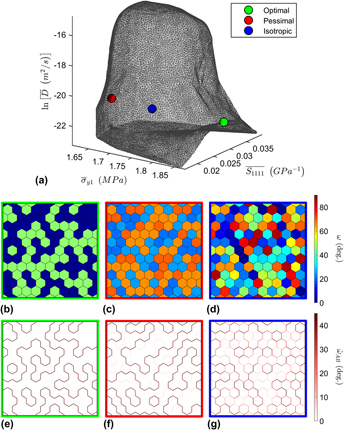
FIG. 5. (a) The properties closure, ${\cal P}$
, for the present design problem. The locations of the optimal, pessimal, and isotropic solutions are also shown. (b)–(d) Microstructures representative of the optimal, pessimal, and isotropic solutions, respectively, with the grains colored according to their crystallographic orientation, ω (see color bar at right). (e)–(f) The grain boundary networks of the corresponding microstructures in (b)–(d), with grain boundaries colored according to their disorientation,
${\cal P}$
, for the present design problem. The locations of the optimal, pessimal, and isotropic solutions are also shown. (b)–(d) Microstructures representative of the optimal, pessimal, and isotropic solutions, respectively, with the grains colored according to their crystallographic orientation, ω (see color bar at right). (e)–(f) The grain boundary networks of the corresponding microstructures in (b)–(d), with grain boundaries colored according to their disorientation, ${\hat \omega _{AB}}$
(see color bar at right).
${\hat \omega _{AB}}$
(see color bar at right).
B. Solving the design problem
With both the microstructural design space $\hbox({\cal M}_{\rm{H}}^{\left( 1 \right)}\hbox)$
and the corresponding properties design space (
$\hbox({\cal M}_{\rm{H}}^{\left( 1 \right)}\hbox)$
and the corresponding properties design space ( ${\cal P}$
) in hand, the solution of our design problem involves identifying the point in
${\cal P}$
) in hand, the solution of our design problem involves identifying the point in ${\cal P}$
that optimally satisfies the design objectives [Eq. (1)] and finding the corresponding microstructure(s) in
${\cal P}$
that optimally satisfies the design objectives [Eq. (1)] and finding the corresponding microstructure(s) in ${\cal M}_{\rm{H}}^{\left( 1 \right)}$
. To do this, we first express the design problem as an optimization problem:
${\cal M}_{\rm{H}}^{\left( 1 \right)}$
. To do this, we first express the design problem as an optimization problem:
 $$\eqalign{ & \mathop {\arg \;\min }\limits_{{\bi p} \in {\bi M}_{\rm{H}}^{\left( 1 \right)} } \quad h\left( {\bi p} \right) \cr & {\rm{subject}}\,{\rm{to}}\,y = 0 \cr}$$
where the objective function is defined by
 $$h\left( {\bi p} \right) = {{z\left( {\bi p} \right) + 2} \over {x\left( {\bi p} \right) + 2}}$$
and the problem has been centered and scaled according to the following coordinate transformations:
 $$x\left( {\,\bi p} \right) = {{2\overline {{{\rm{\sigma }}_{y1}}} \left( {\,\bi p} \right) - \left( {{\rm{max}}\left( {\overline {{{\rm{\sigma }}_{y1}}} } \right) + {\rm{min}}\left( {\overline {{{\rm{\sigma }}_{y1}}} } \right)} \right)} \over {{\rm{max}}\left( {\overline {{{\rm{\sigma }}_{y1}}} } \right) - {\rm{min}}\left( {\overline {{{\rm{\sigma }}_{y1}}} } \right)}}$$
 $$y\left( {\,\bi p} \right) = {{2\overline {{S_{1111}}} \left( {\,\bi p} \right) - \left( {{\rm{max}}\left( {\overline {{S_{1111}}} } \right) + {\rm{min}}\left( {\overline {{S_{1111}}} } \right)} \right)} \over {{\rm{max}}\left( {\overline {{S_{1111}}} } \right) - {\rm{min}}\left( {\overline {{S_{1111}}} } \right)}}$$
 $$z\left( {\,\bi p} \right) = {{2\,{\rm{ln}}\,\overline D\left( {\,\bi p} \right) - \left( {{\rm{max}}\left( {{\rm{ln}}\,\overline D} \right) + {\rm{min}}\left( {{\rm{ln}}\,\overline D} \right)} \right)} \over {{\rm{max}}\left( {{\rm{ln}}\,\overline D} \right) - {\rm{min}}\left( {{\rm{ln}}\,\overline D} \right)}}$$
The theoretical minimum and maximum values of each of the properties appearing in Eq. (42) are provided in Table I. The optimization constraint y = 0 is just the design constraint of Eq. (1b) transformed according to Eq. (42b), where we have chosen $S_{1111}^{{\rm{sub}}} = 2.81 \times {10^{ - 11}}\,{\rm{P}}{{\rm{a}}^{ - 1}}$
.
$S_{1111}^{{\rm{sub}}} = 2.81 \times {10^{ - 11}}\,{\rm{P}}{{\rm{a}}^{ - 1}}$
.
TABLE I. The theoretical maximum and minimum values of each of the three effective properties considered.

Equation (41) indicates that we have chosen the Dirac representation of the texture hull, $M_{\rm{H}}^{\left( 1 \right)}$
, as the optimization domain, with the Dirac ODF coefficients,
p
= (p
1, p
2, … , p
L
), as the optimization variables. Our design problem involves texture sensitive properties,
$M_{\rm{H}}^{\left( 1 \right)}$
, as the optimization domain, with the Dirac ODF coefficients,
p
= (p
1, p
2, … , p
L
), as the optimization variables. Our design problem involves texture sensitive properties, $\overline {{{\rm{\sigma }}_{y1}}}$
and
$\overline {{{\rm{\sigma }}_{y1}}}$
and $\overline {{S_{1111}}}$
, and a grain boundary network sensitive property,
$\overline {{S_{1111}}}$
, and a grain boundary network sensitive property, $\overline D$
. To obtain a self-consistent design solution (i.e., a texture and grain boundary network that are compatible) we must optimize them simultaneously and this requires a relationship between ODF and TJDF. Equation (20) provides the needed relationship between the Fourier ODF coefficients and the Fourier TJDF coefficients. Using Eq. (20) we could perform the optimization with the Fourier ODF coefficients as the design variables and
$\overline D$
. To obtain a self-consistent design solution (i.e., a texture and grain boundary network that are compatible) we must optimize them simultaneously and this requires a relationship between ODF and TJDF. Equation (20) provides the needed relationship between the Fourier ODF coefficients and the Fourier TJDF coefficients. Using Eq. (20) we could perform the optimization with the Fourier ODF coefficients as the design variables and ${\bi c} \in m_{\rm{H}}^{\left( 1 \right)}$
as the domain. However, respecting the bounds of this domain requires the computation of a high-dimensional convex hull,
${\bi c} \in m_{\rm{H}}^{\left( 1 \right)}$
as the domain. However, respecting the bounds of this domain requires the computation of a high-dimensional convex hull, $m_{\rm{H}}^{\left( 1 \right)}$
, which is expensive. In contrast, the texture hull in the Dirac representation,
$m_{\rm{H}}^{\left( 1 \right)}$
, which is expensive. In contrast, the texture hull in the Dirac representation, $M_{\rm{H}}^{\left( 1 \right)}$
, is an (L − 1)-simplex and, consequently, does not require explicit computation. Instead, restricting our solutions to this domain in the Dirac space—which guarantees that they will be physically realizable—is easily accomplished by requiring 0 ≤ p
l
∀ l and
$M_{\rm{H}}^{\left( 1 \right)}$
, is an (L − 1)-simplex and, consequently, does not require explicit computation. Instead, restricting our solutions to this domain in the Dirac space—which guarantees that they will be physically realizable—is easily accomplished by requiring 0 ≤ p
l
∀ l and $\mathop {\sum_{l = 1}^L {{p_l} = 1} }\nolimits^$
.
$\mathop {\sum_{l = 1}^L {{p_l} = 1} }\nolimits^$
.
To perform the optimization over $M_{\rm{H}}^{\left( 1 \right)}$
requires that we recast our constitutive models in terms of
p
. Introducing Eq. (4) into Eqs. (27) and (32) results in:
$M_{\rm{H}}^{\left( 1 \right)}$
requires that we recast our constitutive models in terms of
p
. Introducing Eq. (4) into Eqs. (27) and (32) results in:
 $$\overline {{\rm{\sigma }}_{y1} } = 2{\rm{\pi \tau }}_{{\rm{CRSS}}} \sum\limits_{l = 1}^L {\mathop {p_l\, }\nolimits^l {\rm{\sigma }}_{{\rm{y1}}} } \quad ,$$
 $$\overline {S_{1111} } = 2{\rm{\pi }}\sum\limits_{l = 1}^L {\mathop {p_l\, }\nolimits^l S_{1111} } \quad ,$$
where l σ y1 and l S 1111 are the properties of the l-th fundamental orientation. Our model for grain boundary network diffusivity is already in terms of Dirac coefficients [Eq. (39)], but they are the coefficients of the TJDF. Equation (20) provides a relationship between ODF and TJDF coefficients in the Fourier basis. The corresponding relationship in the Dirac basis is given by:
 $$\tilde \phi _n = \sum\limits_{\left( {a,b,c} \right) \in E_n } {p_a p_b p_c } \quad .$$
In Eq. (45), E
n
is the equivalence class of the n-th fundamental triple junction, (
n
ω12,
n
ω23), defined by the combination of crystal symmetry and triple junction symmetry [Eq. (9)]. In other words, Eq. (45) indicates that the probability of observing a triple junction belonging to a bin centered at (
n
ω12,
n
ω23) is given by the joint probability of observing the corresponding triplet of orientations, summed over all orientation triplets that could produce that triple junction. Substituting Eq. (45) into Eq. (39) permits the computation of $\bar D$
from the Dirac ODF coefficients.
$\bar D$
from the Dirac ODF coefficients.
With all of our constitutive equations in terms of p , it is now possible to solve our design problem in a self-consistent fashion. Equation (40) is of the form of a canonical quasi-convex optimization problem, and we employ sequential quadratic programming to obtain a solution.
Figure 5 shows the optimal solution, together with the pessimal (i.e., worst performing) and isotropic solutions for comparison. The properties closure shown in Fig. 5(a) highlights the competing nature of our design objectives: no microstructure exists for which $\overline {{{\rm{\sigma }}_{y1}}}$
and
$\overline {{{\rm{\sigma }}_{y1}}}$
and $\bar D$
are, respectively, maximized and minimized simultaneously. The optimal microstructure for the design problem is the one that makes the best trade-off between the two competing properties.
$\bar D$
are, respectively, maximized and minimized simultaneously. The optimal microstructure for the design problem is the one that makes the best trade-off between the two competing properties.
With respect to $\overline {{{\rm{\sigma }}_{y1}}}$
, the optimal solution outperforms the pessimal and isotropic solutions by 16% and 10%, respectively. This performance improvement is particularly noteworthy as the maximum theoretical yield strength,
$\overline {{{\rm{\sigma }}_{y1}}}$
, the optimal solution outperforms the pessimal and isotropic solutions by 16% and 10%, respectively. This performance improvement is particularly noteworthy as the maximum theoretical yield strength, ${\rm{max}}\left( {\overline {{{\rm{\sigma }}_{y1}}} } \right)$
, is only 20% larger than the minimum theoretical yield strength,
${\rm{max}}\left( {\overline {{{\rm{\sigma }}_{y1}}} } \right)$
, is only 20% larger than the minimum theoretical yield strength, ${\rm{min}}\left( {\overline {{{\rm{\sigma }}_{y1}}} } \right)$
. Thus, the improvement of the optimal microstructure over the pessimal spans nearly the complete range of possible yield strengths, and the improvement over the isotropic microstructure spans half of the theoretically possible range. The ODF of the optimal solution is dominated by two texture components (orientations): ωA = 0° and ωB = 45°. The ODF of the pessimal solution is identical, but is shifted by a 22.5° rotation (phase shift), which leads to its diminished
${\rm{min}}\left( {\overline {{{\rm{\sigma }}_{y1}}} } \right)$
. Thus, the improvement of the optimal microstructure over the pessimal spans nearly the complete range of possible yield strengths, and the improvement over the isotropic microstructure spans half of the theoretically possible range. The ODF of the optimal solution is dominated by two texture components (orientations): ωA = 0° and ωB = 45°. The ODF of the pessimal solution is identical, but is shifted by a 22.5° rotation (phase shift), which leads to its diminished $\overline {{{\rm{\sigma }}_{y1}}}$
.
$\overline {{{\rm{\sigma }}_{y1}}}$
.
The value of $\overline D$
is the same for both the optimal and pessimal microstructures, and only slightly lower for the isotropic microstructure. The reason that
$\overline D$
is the same for both the optimal and pessimal microstructures, and only slightly lower for the isotropic microstructure. The reason that $\bar D$
is identical for the optimal and pessimal solutions is that they both possess the same TJDF—evident in the visual similarity of their grain boundary networks [Figs. 5(e) and 5(f)]—which are composed entirely of J
1 and J
3 type triple junctions. This is because, as indicated in Eq. (22), two ODFs that differ only by a rotation will possess identical TJDFs. All three microstructures possess the same fraction of low-angle grain boundaries (p
1 = 0.5), but the isotropic microstructure contains J
0 and J
2 type triple junctions, which are not present in the other two microstructures. This highlights the important fact that specification of the fraction of “special” boundaries, p
1, in a microstructure, is insufficient to adequately quantify the structure of the grain boundary network as topological details have a strong effect on its effective properties.
$\bar D$
is identical for the optimal and pessimal solutions is that they both possess the same TJDF—evident in the visual similarity of their grain boundary networks [Figs. 5(e) and 5(f)]—which are composed entirely of J
1 and J
3 type triple junctions. This is because, as indicated in Eq. (22), two ODFs that differ only by a rotation will possess identical TJDFs. All three microstructures possess the same fraction of low-angle grain boundaries (p
1 = 0.5), but the isotropic microstructure contains J
0 and J
2 type triple junctions, which are not present in the other two microstructures. This highlights the important fact that specification of the fraction of “special” boundaries, p
1, in a microstructure, is insufficient to adequately quantify the structure of the grain boundary network as topological details have a strong effect on its effective properties.
VII. SUMMARY
The present work represents the first application of the MSDPO methodology Reference Adams, Henrie, Henrie, Lyon, Kalidindi and Garmestani6,Reference Adams, Kalidindi and Fullwood7 to a defect sensitive property (grain boundary network diffusivity). The mathematical apparatus required for this development was presented and applied to a specific design problem to illustrate its utility.
We have defined the TJDF for two-dimensional crystallographic textures as a means to quantify the structure of the grain boundary network. We also provided the equivalence relations for triple junction symmetries and explicitly defined the boundaries of a triple junction fundamental zone that includes the effects of both triple junction symmetry and crystallographic symmetry. A formula was derived relating crystallographic texture (ODF) to grain boundary network topology (TJDF) and, by inverting this relationship, we demonstrated that it is possible to recover an ODF from a given TJDF modulo a rotation operation. Using the spectral representation of the ODF and TJDF, we constructed microstructure hulls, in both the Fourier and Dirac bases, which constitute the complete universe of possible ODFs and TJDFs, respectively.
Using these tools, we performed a design case study for a flexible electronics application, with competing design constraints/objectives, to demonstrate the process of texture mediated grain boundary network design. We determined a grain boundary network and commensurate texture that optimally satisfy the design objectives, which included elastic, plastic (initial yield), and kinetic properties. In the process we also developed a refined constitutive model for grain boundary network diffusivity that considers the influence of grain boundary network topology. The shape of the resulting properties closure indicated a non-trivial correlation between the properties considered, which required a trade-off between yield strength and diffusivity. The improvement in yield strength of the optimal microstructure over an isotropic microstructure was fully half of the theoretically possible range without significant sacrifice in diffusivity. The generalization of the present work to arbitrary 3D textures will be presented in a subsequent paper.
We note that the anisotropy ratio of aluminum is nearly unity and therefore the design space for elastic properties in our case study was limited. However, the focus of the present work was on the novel ability to explore the design space for grain boundary network sensitive properties, specifically diffusivity as it pertains to electromigration in metallic interconnects. Aluminum was chosen because of its relevance to the electronic application and because it is not amenable to traditional cyclic thermomechanical processing, commonly referred to as grain boundary engineering (GBE). While GBE has demonstrated substantial improvements in materials properties by modifying the structure of the grain boundary network, it is only effective for low stacking-fault energy FCC metals. The present work provides a way to identify optimal grain boundary network structures for arbitrary polycrystalline materials, thereby facilitating a route to grain boundary engineer a much broader class of materials, including those, like aluminum, that do not readily form annealing twins.
Once an optimal microstructure is found, the next challenge is to identify a suitable processing route to synthesize it. While this remains a challenging problem, the texture mediated approach to grain boundary network design outlined in the present work suggests a potential strategy. The influence of various processing methods on crystallographic texture has been studied extensively. If these operations can be combined in an appropriate sequence it may be possible to approach a target texture. With the relationship between texture and grain boundary network structure, identified in the present work, this may enable the synthesis of desired grain boundary network structures also. Some work on the construction of suitable processing paths for synthesizing desired textures has already been performed Reference Shaffer, Knezevic and Kalidindi45 and merits further investigation.
ACKNOWLEDGMENTS
This work was supported by the US Department of Energy (DOE), Office of Basic Energy Sciences under award no. DE–SC0008926. O.K.J. acknowledges support from the Department of Defense (DoD) through the National Defense Science & Engineering Graduate Fellowship (NDSEG) Program.
APPENDIX A: PROPERTIES OF THE TJDF AND ITS COEFFICIENTS
Appendix A.1: The TJDF coefficients
The Fourier coefficients of a TJDF in the present two-dimensional case are computed via
 $$\mathop {{t_{{k_1}}^{{k_3}} = {1 \over {4{{\rm{\pi }}^2}}}\int_{\rm{0}}^{2{\rm{\pi }}} {\int_{\rm{0}}^{2{\rm{\pi }}} {T\left( {{{\rm{\omega }}_{12}},{{\rm{\omega }}_{23}}} \right){{\rm{e}}^{ - i{k_1}{\omega _{12}}}}{{\rm{e}}^{ - i{k_3}{{\rm{\omega }}_{23}}}}{\rm{d}}{{\rm{\omega }}_{12}}{\rm{d}}{{\rm{\omega }}_{{\rm{23}}}}} } \quad .$$
We take the convention that the TJDF is normalized over the entirety of S 1 × S 1, which sets
 $$t_0^0 = {1 \over {4{{\rm{\pi }}^2}}}\quad .$$
Because a TJDF is a real-valued function we have that T*(ω12, ω23) = T(ω12, ω23). Expressing both sides of this equation in spectral form [Eq. (5)] and rearranging, one arrives at the reality condition for the coefficients of a TJDF:
 $$\mathop {{t_{{k_1}}^{{k_3}{\rm{*}}} = \mathop {{t_{ - {k_1}}^{ - {k_3}} \quad .$$
Appendix A.2: Triple junction symmetry relations
The physical symmetries of a triple junction were expressed in the form of the equivalence relations provided in Eq. (9). These equivalence relations induce constraints on the coefficients of a TJDF, which limit the number of independent coefficients that must be calculated. Consider the equivalence relation of Eq. (9f), which requires that the value of a TJDF at the point (ω12, ω23) be equal to the value of the TJDF at point (−ω23, −ω12). This implies
 $$T\left( {{{\rm{\omega }}_{12}},{{\rm{\omega }}_{23}}} \right) = T\left( { - {{\rm{\omega }}_{23}}, - {{\rm{\omega }}_{12}}} \right)\quad .$$
Expressing the TJDF in spectral form we have
 $$\sum\limits_{k_1 ,k_3 } {\mathop {t_{k_1 } ^{k_3 } {\rm{e}}^{ik_1 {\rm{\omega }}_{12} } {\rm{e}}^{ik_3 {\rm{\omega }}_{23} } } = \sum\limits_{k_1^\prime ,k_3^\prime } {\mathop {t_{k_1^\prime } ^{k_3^\prime } {\rm{e}}^{ - ik_1^\prime {\rm{\omega }}_{23} } {\rm{e}}^{ - ik_3^\prime {\rm{\omega }}_{12} } }$$
using the index substitution $- k_3^\prime \leftrightarrow k_1^\prime$
on the right-hand side and rearranging we find
$- k_3^\prime \leftrightarrow k_1^\prime$
on the right-hand side and rearranging we find
 $$\sum\limits_{k_1 ,k_3 } {\mathop {t_{k_1 } ^{k_3 } {\rm{e}}^{ik_1 {\rm{\omega }}_{12} } {\rm{e}}^{ik_3 {\rm{\omega }}_{23} } } = \sum\limits_{k_1^\prime ,k_3^\prime } {\mathop {t_{ - k_3^\prime } ^{ - k_1^\prime } {\rm{e}}^{ik_1^\prime \omega _{12} } {\rm{e}}^{ik_3^\prime {\rm{\omega }}_{23} } }\quad .$$
Equating the coefficients yields the constraint imposed by this equivalence relation:
 $$\mathop {{t_{{k_1}}^{{k_3}} = \mathop {{t_{ - {k_3}}^{ - {k_1}} \quad .$$
The same process may be followed for each of the equivalence relations of Eq. (9), resulting in the following set of TJDF coefficients whose values must be equal for the TJDF to exhibit the required physical symmetries of triple junctions:
 $$\mathop {{t_{{k_1}}^{{k_3}} = \mathop {{t_{{k_3} - {k_1}}^{ - {k_1}} = \mathop {{t_{ - {k_3}}^{{k_1} - {k_3}} = \mathop {{t_{{k_3} - {k_1}}^{{k_3}} = \mathop {{t_{{k_1}}^{{k_1} - {k_3}} = \mathop {{t_{ - {k_3}}^{ - {k_1}} \quad .$$
Appendix A.3: Crystal symmetry relations
In addition to triple junction symmetries, the TJDF must exhibit crystallographic symmetries that are inherited from the crystal symmetries of the grains coordinating the triple junction. These symmetries also impose constraints on the TJDF coefficients. If the grains in this two-dimensional case possess cyclic symmetry of order s, then we have that
 $${\rm{\omega }} \,\sim\, {\rm{\omega }} + k{{\rm{\omega }}_s}\quad ,$$
where ω s ≡ 2π/s and k ∈ ℤ. Substituting this into the definition of a misorientation yields.
 $$\eqalign{ & {{\rm{\omega }}_{{\rm{AB}}}} = {{\rm{\omega }}_{\rm{B}}} - {{\rm{\omega }}_{\rm{A}}} \cr & <$$><$$>= \left( {{{\rm{\omega }}_{\rm{B}}} + k{{\rm{\omega }}_s}} \right) - \left( {{{\rm{\omega }}_{\rm{A}}} + l{{\rm{\omega }}_s}} \right) {\cr & <$$><$$>= {{\rm{\omega }}_{\rm{B}}} - {{\rm{\omega }}_{\rm{A}}} + \left( {k - l} \right){{\rm{\omega }}_s} \cr & <$$><$$>= {{\rm{\omega }}_{{\rm{AB}}}} + \left( {k - l} \right){{\rm{\omega }}_s} \cr & \cr}$$
Because (k − l) ∈ ℤ, this implies that the misorientations exhibit independent periodicity equal to ω s , i.e.,
 $${{\rm{\omega }}_{{\rm{AB}}}} \,\sim\, {{\rm{\omega }}_{{\rm{AB}}}} + m{{\rm{\omega }}_s}\quad .$$
Following the same process as before we can substitute Eq. (A11) into the TJDF to determine the constraints on the TJDF coefficients. The result is
 $$\mathop {{t_{{k_1}}^{{k_3}} = \mathop {{t_{{k_1}}^{{k_3}} {{\rm{e}}^{i\left( {{k_1}m + {k_3}n} \right){{\rm{\omega }}_s}}}\quad ,$$
where m,n ∈ ℤ. For this expression to be valid, either $\mathop {{t_{{k_1}}^{{k_3}} = 0$
(the trivial case), or we must have that k
1
m + k
3
n is an integer multiple of s for arbitrary m and n, which is only possible if k
1 and k
3 are both integer multiples of s. Thus, the crystal symmetry constraint for the TJDF coefficients is
$\mathop {{t_{{k_1}}^{{k_3}} = 0$
(the trivial case), or we must have that k
1
m + k
3
n is an integer multiple of s for arbitrary m and n, which is only possible if k
1 and k
3 are both integer multiples of s. Thus, the crystal symmetry constraint for the TJDF coefficients is
 $$\mathop {t_{k_1 } ^{k_3 } = 0\,\forall \,k_1 ,k_3 \, \notin \,sℤ\quad {\rm{.}}$$
APPENDIX B: DERIVATION OF THE INVERSE MAPPING FROM TJDF TO ODF
The forward mapping from ODF to TJDF for two-dimensional textures is accomplished in the same fashion as for the three-dimensional case provided in Ref. Reference Johnson and Schuh21. If grain orientations are spatially uncorrelated, then the joint probability density for observing a triple junction coordinated by orientations ω1, ω2, and ω3 is given by
 $$\tilde T\left( {{{\rm{\omega }}_1},{{\rm{\omega }}_2},{{\rm{\omega }}_3}} \right) = f\left( {{{\rm{\omega }}_1}} \right)f\left( {{{\rm{\omega }}_2}} \right)f\left( {{{\rm{\omega }}_3}} \right)\quad ,$$
where f(ω) is the ODF. Expressing this in spectral form we obtain
 $$\tilde T\left( {{{\rm{\omega }}_1},{{\rm{\omega }}_2},{{\rm{\omega }}_3}} \right) = \sum\limits_{{k_1} = - \infty }^\infty {{c_{{k_1}}}{{\rm{e}}^{i{k_1}{{\rm{\omega }}_1}}}} \sum\limits_{{k_2} = - \infty }^\infty {{c_{{k_2}}}{{\rm{e}}^{i{k_2}{{\rm{\omega }}_2}}}} \sum\limits_{{k_3} = - \infty }^\infty {{c_{{k_3}}}{{\rm{e}}^{i{k_3}{{\rm{\omega }}_3}}}} \quad .$$
Using the definition of a misorientation, ωAB = ωB − ωA, and making use of the addition theorem for exponentials, the joint probability density function can be expressed in terms of the two independent misorientations according to
 $$\tilde T\left( {{{\rm{\omega }}_{12}},{{\rm{\omega }}_{23}}} \right) = \sum\limits_{{k_1},{k_2},{k_3}} {{c_{{k_1}}}{c_{{k_2}}}{c_{{k_3}}}{{\rm{e}}^{ - i{k_1}{{\rm{\omega }}_{12}}}}{{\rm{e}}^{i{k_3}{{\rm{\omega }}_{23}}}}} \int_0^{2{\rm{\pi }}} {{{\rm{e}}^{i\left( {{k_1} + {k_2} + {k_3}} \right){{\rm{\omega }}_2}}}{\rm{d}}{{\rm{\omega }}_2}} \quad .$$
The integral evaluates to zero unless k 2 = −(k 1 + k 3), for which its value is 2π, which eliminates the summation over k 2. The resulting uncorrelated TJDF is given by
 $$\tilde T\left( {{{\rm{\omega }}_{12}},{{\rm{\omega }}_{23}}} \right) = \sum\limits_{{k_1},{k_3}} {\mathop {{{\tilde t}_{{k_1}}^{{k_3}} {{\rm{e}}^{i{k_1}{{\rm{\omega }}_{12}}}}{{\rm{e}}^{i{k_3}{{\rm{\omega }}_{23}}}}}$$
with the TJDF coefficients given by
 $$\mathop {{{\tilde t}_{{k_1}}^{{k_3}} = 2{\rm{\pi }}c_{{k_1}}^{\rm{*}}{c_{{k_1} - {k_3}}}{c_{{k_3}}}\quad ,$$
which is the expression given in Eq. (20) defining the mapping from ODF to TJDF via their respective Fourier coefficients.
To obtain the inverse mapping, note that the ODF coefficients and the TJDF coefficients are only nonzero when their indices are integer multiples of s. Let k 1 = s, k 3 = ηs, where η ∈ ℤ, and substitute (c 0)−1 for 2π; Eq. (B5) then becomes
 $$\mathop {{{\tilde t}_s}}\nolimits\!\!^{\eta s} = {{c_s^{\rm{*}}{c_{\left( {1 - \eta } \right)s}}{c_{\eta s}}} \over {{c_0}}}\quad .$$
Solving for c ηs and using the complex conjugation relation, c −k = c k *, we obtain
 $${c_{\eta s}} = {{{c_0}\mathop {{{\tilde t}_s}}\nolimits\!\!^{\eta s} } \over {c_s^{\rm{*}}c_{\left( {\eta - 1} \right)s}^{\rm{*}}}}\quad ,$$
which is in the form of a recurrence relation: given the TJDF coefficients and c
(η−1)s
it is possible to compute c
ηs
. To use Eq. (B7) one must know the value of c
s
. This is obtained by noting that if k
1 = k
3 = s then Eq. (B5) yields $\mathop {{{\tilde t}_s}}\nolimits\!^s = c_s^{\rm{*}}{c_s}$
, which is just the squared magnitude of c
s
. Therefore,
$\mathop {{{\tilde t}_s}}\nolimits\!^s = c_s^{\rm{*}}{c_s}$
, which is just the squared magnitude of c
s
. Therefore, $\mathop {{{\tilde t}_s}}\nolimits\!^s$
must be a non-negative real number and the magnitude of c
s
is given by
$\mathop {{{\tilde t}_s}}\nolimits\!^s$
must be a non-negative real number and the magnitude of c
s
is given by
 $$\left\| {{c_s}} \right\| = \sqrt {\mathop {{{\tilde t}_s}}\nolimits\!^s } \quad .$$
The phase of c s is a free parameter and cannot be recovered, but can be arbitrarily chosen without loss of generality. This indicates that the coefficients of an ODF may be recovered from those of an uncorrelated TJDF, modulo a rotation operation and, conversely, in the absence of spatial correlations in grain orientation, all ODFs that differ by only a rotation will yield the same TJDF.
A closed form solution for the recurrence relation can be obtained by evaluating Eq. (B7) for increasing values of η and simplifying the results. We omit the details of this straightforward, but tedious, process and present the final result:
 $${c_{\eta s}} = \left\{ {\matrix{ {{c_0}\prod\limits_{j = 1}^{{\eta \mathord{\left/ {\vphantom {\eta 2}} \right. \kern-\nulldelimiterspace} 2}} {{{\tilde t_s^{\left( {2j} \right)s}} \over {\tilde t_{\left( {2j - 1} \right)s}^s}}} } & {{\rm{for}}\;{\mathop{\rm even}\nolimits} \,\eta } \cr {{c_s}\prod\limits_{j = 1}^{{{\left( {\eta - 1} \right)} \mathord{\left/ {\vphantom {{\left( {\eta - 1} \right)} 2}} \right. \kern-\nulldelimiterspace} 2}} {{{\tilde t_s^{\left( {2j + 1} \right)s}} \over {\tilde t_{\left( {2j} \right)s}^s}}} } & {{\rm{for}}\;{\mathop{\rm odd}\nolimits} \,\eta } \cr} } \right.$$
which permits the computation of the ODF coefficients directly from those of the uncorrelated TJDF without resorting to recurrence.


