


1 Introduction
Air temperature inversion, a situation in which atmospheric temperature increases with height, is a common feature in the Arctic planetary boundary layer (Kahl, Reference Kahl1990; Mernild and Liston, Reference Mernild and Liston2010; Shahi and others, Reference Shahi, Abermann, Heinrich, Prinz and Schöner2020). Such inversions create stable layers of air that have multiple consequences for the Arctic environment. They impact vertical gradients of flora and fauna and have a direct effect on physical characteristics such as permafrost thaw depths and snow cover. Comprehensive knowledge of the spatial and temporal variability of temperature inversions is therefore crucial for ice and snow melt calculations (Chutko and others, Reference Chutko, Lamoureux and Shea2009), glacier mass-balance estimates (Hulth and others, Reference Hulth, Rolstad, Trondsen and Rødby2010; Mernild and Liston, Reference Mernild and Liston2010; Mernild and others, Reference Mernild, Beckerman, Knudsen, Hasholt and Yde2018), water resource assessments (Archer, Reference Archer2004) and pollutant concentrations and pathways (Kukkonen and others, Reference Kukkonen2005; Kerminen and others, Reference Kerminen2007).
For this reason, many studies have focused on the quantification of spatial and temporal variability of inversion in the Arctic (Kahl, Reference Kahl1990; Serreze and others, Reference Serreze, Kahl and Schnell1992; Mernild and Liston, Reference Mernild and Liston2010; Zhang and others, Reference Zhang, Seidel, Golaz, Deser and Tomas2011; Shahi and others, Reference Shahi, Abermann, Heinrich, Prinz and Schöner2020). Nevertheless, atmospheric vertical sounding data are sparse due to the generally rough terrain, difficulty of access and logistical constraints (Mernild and Liston, Reference Mernild and Liston2010). Most of the aforementioned studies employed measurements from the few existing radiosonde stations or modeled reanalysis data for their research.
Using radiosonde data for the analysis of temperature inversions in the Arctic has certain advantages, such as long time-series and high accuracy, but alongside the benefits of relatively inexpensive and continuous data collection, there are, however, several challenges (Gilson and others, Reference Gilson, Jiskoot, Cassano, Gultepe and James2018b). One is the limited vertical resolution, as a result of which many of the shallower or near-surface inversions are not captured by the radiosonde data (Tjernström, Reference Tjernström2005; Mernild and Liston, Reference Mernild and Liston2010; Vihma and others, Reference Vihma2011; Fochesatto, Reference Fochesatto2015; Palo and others, Reference Palo, Vihma, Jaagus and Jakobson2017). Furthermore, radiosonde data are not well suited to the analysis of diurnal or spatial changes in the atmosphere because of the low temporal resolution (typically not more than twice a day) and spatial distribution (particularly in the Arctic, radiosonde launching sites may often be hundreds of km apart) of the data. Radiosonde data collected during scientific cruises in the Arctic have higher vertical and spatial resolution and are collected by more precise instruments than stationary ones, but they only exist episodically (Tjernström and others, Reference Tjernström2014; Gilson and others, Reference Gilson, Jiskoot, Cassano, Gultepe and James2018b). Compared to radiosonde, modeled reanalysis data provide a higher horizontal and vertical resolution, represent a spatially and temporally coherent dataset, and cover long time periods, opening up new possibilities in Arctic temperature inversion research. However, limitations include the low resolution in the lowest meters of the data, which limits the applicability to resolving complex low tropospheric conditions and processes (Tjernström and Graversen, Reference Tjernström and Graversen2009; Medeiros and others, Reference Medeiros, Deser, Tomas and Kay2011; Palarz and others, Reference Palarz, Luterbacher, Ustrnul, Xoplaki and Celiński-Mysław2020). Cold or warm biases have been detected in the surface or near-surface reanalysis data, which can lead to incorrect quantification of temperature inversion characteristics (Wesslén and others, Reference Wesslén2014; Graham and others, Reference Graham, Hudson and Maturilli2019; Tetzner and others, Reference Tetzner, Thomas and Allen2019; Palarz and others, Reference Palarz, Luterbacher, Ustrnul, Xoplaki and Celiński-Mysław2020).
Compared to other locations in Greenland, scientific investigations have a long history in Sermilik, starting in 1933 (Hasholt and others, Reference Hasholt, van As and Knudsen2016). Several studies conducted in this area have addressed and quantified temperature inversions (Mernild and others, Reference Mernild, Hansen, Jakobsen and Hasholt2008; Mernild and Liston, Reference Mernild and Liston2010; Hasholt and others, Reference Hasholt, van As and Knudsen2016; Gilson and others Reference Gilson, Jiskoot, Cassano and Nielsen2018a, Reference Gilson, Jiskoot, Cassano, Gultepe and James2018b). However, to analyze temperature inversions most of these studies used radiosonde data, which is subject to the aforementioned limitations.
Temperature inversions affect glacier mass-balance gradients (Hulth and others, Reference Hulth, Rolstad, Trondsen and Rødby2010; Mernild and Liston, Reference Mernild and Liston2010; Mernild and others, Reference Mernild, Beckerman, Knudsen, Hasholt and Yde2018) and a number of studies have observed increased sea ice and glacier melt in the presence of temperature inversions (Chutko and others, Reference Chutko, Lamoureux and Shea2009; Tjernström and others, Reference Tjernström2015). However, understanding the complex relationship between temperature inversions and glacier ablation remains difficult and requires further research. The recent development of small, lightweight and low-cost unoccupied aerial vehicles (UAVs) equipped with meteorological sensors open up new opportunities for (micro-)meteorological measurements (Elston and others, Reference Elston2015; Villa and others, Reference Villa, Gonzalez, Miljievic, Ristovski and Morawska2016; Kral and others, Reference Kral2018; Kimball and others, Reference Kimball, Montalvo and Mulekar2020; Tikhomirov and others, Reference Tikhomirov, Lesins and Drummond2021; Pina and Vieira, Reference Pina and Vieira2022). The advantages of UAV-based measurements include low operating costs per single atmospheric profile, fine vertical resolution, spatial flexibility, good control over flight parameters, less manpower, ease of operation and low environmental impact.
All these advantages are crucial for the exploration of the atmospheric boundary layer in polar regions, which has already been confirmed by various studies. Cassano (Reference Cassano2014) used UAVs to observe atmospheric temperature trends near McMurdo Station, Antarctica, for 4 d in January and September 2012. Kral and others (Reference Kral2018) probed the atmospheric column from the surface to an altitude of 1800 m with different UAVs during 3 weeks in February 2017 over sea ice in Finland. Also, Tikhomirov and others (Reference Tikhomirov, Lesins and Drummond2021) investigated the suitability of UAVs to observe the Arctic planetary boundary layer in February to March in Nunavut, Canada. All these studies were able to measure the vertical stratification during different meteorological situations in a high vertical resolution, proving the suitability of UAVs as a tool to gain more insight into the dynamics and properties of the atmosphere. The present study aims to add onto this by using UAV-based meteorological measurements in order to analyze and better understand the spatio-temporal variations of air temperature inversions in the Mittivakkat valley in southeast Greenland and their possible impact on the surface mass balance of the Mittivakkat Gletsjer.
2 Study area
The Mittivakkat valley is located in the southwestern part of Ammassalik Island in southeast Greenland (Fig. 1). Near the coast, it has a width of about 300 m and becomes narrower toward the glacier (~200–150 m). The name of the area is derived from Mittivakkat Gletsjer, a local temperate glacier. The glacier is ~5.5 km long, has an average thickness of 90 m and covers an elevation range between 160 and 880 m a.s.l. and an area of 15.8 km2. The glacier has been retreating since the end of the Little Ice Age (~1900 AD) and since 1996, ELA has risen from 500 m a.s.l. to 730 m a.s.l. (average for 1996–10) (Yde and others, Reference Yde2014).

Fig. 1. Top: Location of the study area (black dot in the overview map) with the Sermilik research station (red dot, letter A), ablation stakes (yellow dots), AWS (blue triangles), the course of the transect (blue line), the prevailing wind direction during the field campaign derived from the respective AWS (green arrow), the locations where the UAV profiles were taken (red dots) and the direction to Tasiilaq (black arrow). Bottom: Conceptual overview of the 2019 field campaign with all AWS and locations where the UAV profiles were taken (Abermann and others, Reference Abermann, Shahi, Hansche and Schöner2019). Outline map of Greenland (Moon and others, Reference Moon, Fisher, Harden and Stafford2021); Basemap: Sentinel-2, 14 July 2019.
The area is characterized by sporadic permafrost, a pronounced alpine relief with elevations spanning from sea level to 1096 m a.s.l. (Humlum and Christiansen, Reference Humlum and Christiansen2008). The climate in the study area is classified as a tundra climate and is strongly influenced by the passage of low pressure systems (e.g. the Icelandic Low) and of the warm Irminger Current (Mernild and Hasholt, Reference Mernild and Hasholt2006; Gilson and others, Reference Gilson, Jiskoot, Cassano and Nielsen2018a). Data from the Automatic Weather Station (AWS) in Tasiilaq for the period 1991–20 show that the mean annual air temperature is $-0.3^\circ$ C, July is the warmest month with a mean temperature of $7.2^\circ$
 C near the coast, and February is the coldest month, with a mean temperature of –$6.1^\circ$
 C. The mean annual precipitation in the study region for this period is ~900 mm, with lower precipitation during the summer (Cappelen and Jensen, Reference Cappelen and Jensen2021). The Mittivakkat valley was chosen for this study because of its long research history, existing infrastructure (Sermilik research station), availability of complementary measurements for this study (e.g. AWS) and prevailing environmental conditions (e.g. spatially highly variable surface characteristics).
3 Data
Radiosonde soundings
The radiosonde data from the nearby Tasiilaq station were accessed through the quality-controlled Integrated Global Radiosonde Archive (IGRA). The station is located ~15 km southeast of the Sermilik research station on a hillside at the upper part of Tasiilaq. The meteorological variables are recorded at specific pressure and other significant thermodynamic levels (Durre and others, Reference Durre, Vose and Wuertz2006; Gilson and others, Reference Gilson, Jiskoot, Cassano and Nielsen2018a). The pressure levels include those specified by the World Meteorological Organization (1000, 925, 850, 700, 500, 400, 300, 250, 200, 150, 100, 70, 50, 30, 20 and 10 hPa) (Isioye and others, Reference Isioye, Combrinck and Botai2016). Soundings are taken twice daily at 10 a.m. and 10 p.m. Only soundings at levels below 500 m a.g.l. were used for the study. Currently, the Vaisala radiosonde RS41 is used at the station in Tasiilaq. According to Vaisala (Reference Vaisala2020), the accuracy is $\pm 0.3^\circ$ C for temperature.
Reanalysis products
We evaluate the performance of three reanalysis products on how well they can represent the lower atmospheric stratification. These are the ERA Interim (ERA-I), ERA5 and the Copernicus Arctic Regional Reanalysis (CARRA). The ERA-I reanalysis is available with $0.7^\circ$ (~80 km in the study area) and the ERA5 with $0.25^\circ$
 (~31 km) horizontal resolution (Palarz and others, Reference Palarz, Celiński-Mysław and Ustrnul2018). While the former products exist on a global scale, CARRA only covers parts of the Arctic and the horizontal resolution is 2.5 km (ECMWF, 2021). From both ERA5 and ERA-I we extracted temperature datasets for all available model levels below 500 m a.g.l. (ERA-I: 10 levels, ERA5: 16 levels). The values from the grid-cells closest to our study area were linearly interpolated to the coordinates of the Sermilik research station. In CARRA, height levels up to 500 m a.g.l. (11 levels) were used and complemented with surface and 2 m air temperatures from the same dataset. For our analysis, the time steps of 10 a.m. and 10 p.m. were used.
The surface elevation in the reanalyses is represented by the surface geopotential height (also called orography) (ECMWF, 2020). The extracted value for the surface elevation is 428 m a.s.l. for the ERA-I model and 151 m a.s.l. for ERA5. In contrast to ERA5 and ERA-I, the CARRA surface elevation is given in m a.s.l. (70 m a.s.l. for the nearest gridpoint to Sermilik research station).
Observations from AWS
Data from four AWS at different elevations were used to assess the changes in the meteorological parameters and to identify general inversion periods. The locations of the AWS are shown in Figure 1. AWSCCMORE was set up on a nunatak for the period 7–14 July 2019, all other AWSs are stationary. Further information about the AWSs used in this study can be found in Hansche (Reference Hansche2021).
4 Methods
UAV soundings
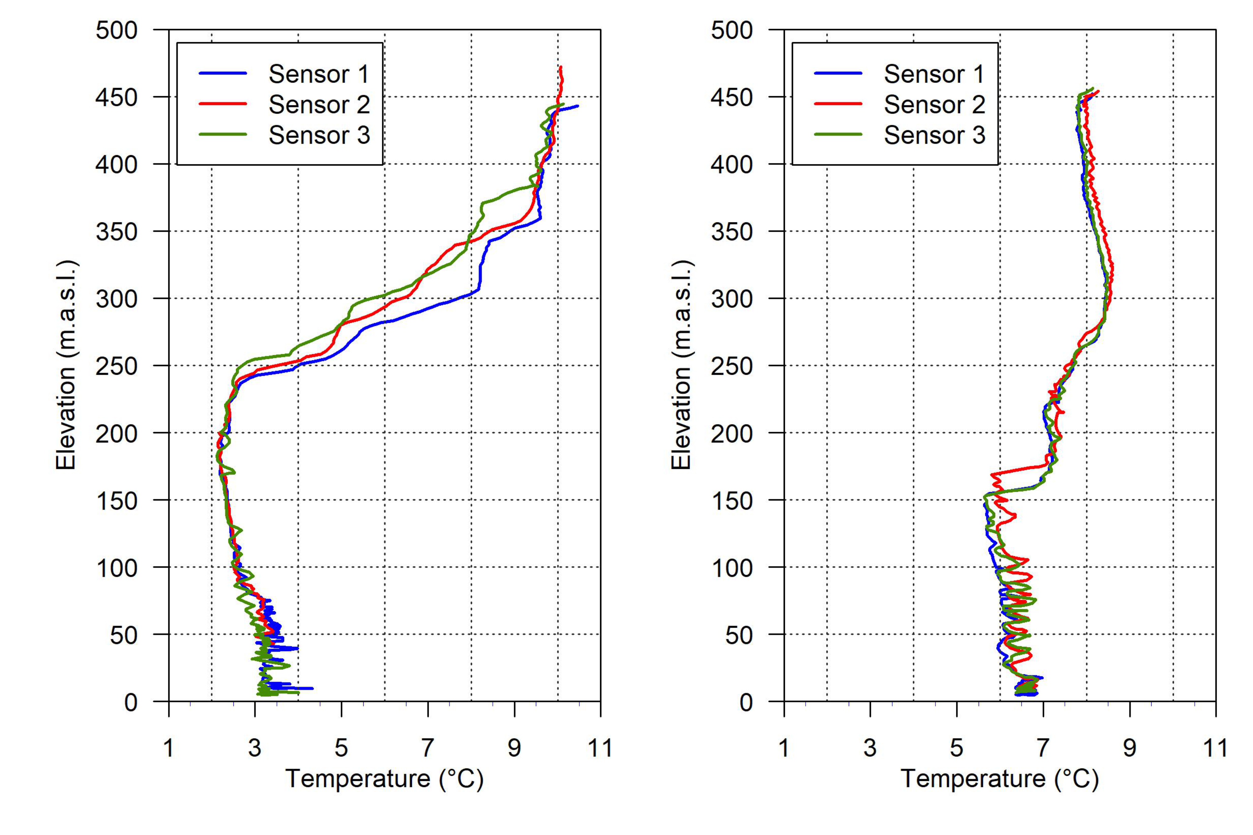
In this study atmospheric variables up to a height of 500 m above ground level (m a.g.l.) were measured using an iMet-XQ2 sensors mounted on commercial low-cost UAVs (DJI MAVIC Pro). A total of three UAVs of the same type equipped with iMet-XQ2 sensors were used, two of which were for the measurements (single measurements and simultaneous measurements at locations B & C and D & E) and one as a backup. The stand-alone sensor with rechargeable power supply independently records temperature, relative humidity, pressure, date, time, altitude and geographic position, with an accuracy of $\pm 0.3^\circ$ C for temperature, $\pm 5\percnt$
 for relative humidity and ±1.5 hPa for pressure with a response time of less than 1 s. Furthermore, the accuracy of the GNSS (GNSS antenna receiver that tracks multiple GNSS systems (GPS, GLONASS, BeiDou and QZSS)) is 8 m horizontally and 12 m vertically (InterMet, 2018). For the further analysis of temperature inversions and their spatio-temporal changes, the collected temperature profiles were analyzed. In order to better understand smaller-scale processes, such as the origin of air masses, relative humidity profiles were also analyzed. In order to ensure adequate ventilation, the iMet-XQ2 was placed on top of the UAV. Since the components that create heat are located in the rear half of the UAV body, the sensor is mounted in the front half in order to avoid artificial sensor heating (Greene and others, Reference Greene, Segales, Waugh, Duthoit and Chilson2018; Kimball and others, Reference Kimball, Montalvo and Mulekar2020). Additionally, iMet-XQ2 has an aluminum coating to reduce the heating effect from terrestrial and solar radiation (Kimball and others, Reference Kimball, Montalvo and Mulekar2020). To investigate the sensor accuracy, two ascents were performed 5 h apart with all three iMet-XQ2 sensors used in this study. In the first ascent, sensor two was placed on top of the UAV and sensors one and three were placed on a string ~35 m below the UAV. During the second ascent, all three sensors were attached to a string 35 m below the UAV. In both ascents, the UAV covered approximately the lowest 450 m a.s.l. All sensors showed similar temperature evolution and differed from each other by an average of $0.2^\circ$
 C in both ascents (RMSE ascent one: $0.4^\circ$
 C; RMSE ascent two: $0.2^\circ$
 C, Fig. S1). The profiles were collected at specific locations, which are marked with the letters A to H in Figure 1 and Table 1. At location A (Sermilik research station), daily measurements at 10 a.m. and 10 p.m. have been taken for comparability with the radiosonde and three reanalysis products (ERA-I, ERA5, CARRA). After the profile was collected at location A at 10 a.m., the locations up (B–H) and back (H–B) were visited, with simultaneous ascents at locations B and C as well as D and E. In contrast to the measurements at A, the profiles at all other locations were not collected at fixed times of the day for practical reasons. Thus, a total of 113 profiles were collected between 7 July 2019 and 18 July 2019 (no profiles were collected along the transect on the first day in the field, 6 July 2019). All UAV profiles were averaged in 12 m steps, which corresponds to the vertical accuracy of the GNSS. Also, the first value of the UAV profiles taken over the glacier was set to $0^\circ$
 C since melt conditions occurred during the entire field period. Furthermore, two humidity sensors broke during fieldwork, the first on 13 July 2019 and the second on 15 July 2019. The profiles acquired with the broken sensors were excluded from later evaluations.
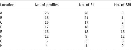
Table 1. Locations and surface properties of the acquisition points

All timestamps used in this study are in UTC-2.
Inversion layer identification and classification
The objective inversion detection algorithm described by Kahl (Reference Kahl1990) was applied to identify temperature inversions and their characteristics in all datasets. The following inversion characteristics were quantified: the inversion base (Z$_{\rm {Base}}$ ) is the elevation at which the temperature starts to increase with height. Inversion top (Z$_{\rm {Top}}$
 ) is the top of the inversion, which is the elevation level at which the temperature starts to decrease. Furthermore, the inversions found were classified as follows: if Z$_{\rm {Base}}$
 started at the surface the inversion is called surface-based inversions (SBI) and inversions with a Z$_{\rm {Base}}$
 above 0 m a.g.l. are called elevated inversions (EI). We use the sensor accuracy ($0.3^\circ$
 C) as a lower threshold of inversion detection and deploy the same for both UAV and radiosonde. For the reanalysis products, we use the threshold >$0^\circ$
 C.
C.
Spatio-temporal interpolation
In order to determine spatial patterns of the valley atmosphere, the UAV profiles were linearly interpolated. Only profiles B to G were used for the spatial interpolations in order to display an along-valley transect of the atmosphere from the sea to AWS$_{\rm {GEUS}}$ on the glacier (Fig. 1). Since the acquisition of profiles along the transect between B and G takes between 1–4 h (for logistical reasons), we relate the spatial patterns obtained in the valley atmosphere to the changes that occurred at AWS$_{\rm {COAST}}$
 during this time period. In order to make the individual interpolated transects comparable, we calculate differences with regard to the average atmospheric variable at AWS$_{\rm {COAST}}$
 during the acquisition of the transect. This is done by taking the difference between the interpolated temperature and humidity profiles and the average value of temperature or relative humidity measured at AWS$_{\rm {COAST}}$
 during the survey period of each transect. This means that if a value in the interpolated transect indicates, e.g. $3^\circ$
 C, this point in the transect is $3^\circ$
 C warmer than the average value measured by AWS$_{\rm {COAST}}$
 throughout the transect acquisition. Furthermore, in order to assess the influence of this extended period and to assess whether it is adequate to interpret the transect as a spatial distribution rather than a temporal evolution, we display the variability of temperature and relative humidity (Figs 3 and 4 density plots) during the period of the transect acquisition between B and G at AWS$_{\rm {COAST}}$
 . Surface topography is determined from GNSS measurements taken along the transect. Only those transects were interpolated where at least four UAV profiles were collected. In total, 12 temperature and nine relative humidity transects were available and interpolated. The lower number of interpolated relative humidity transects is due to the two humidity sensors which broke during the fieldwork. Furthermore, the term transect is used in this study only for the interpolated profiles that lie between location B and G.
Ablation stakes
During the field study, the ice ablation was measured using an existing network of ablation stakes on Mittivakkat Gletsjer (Knudsen and Hasholt, Reference Knudsen and Hasholt2008). Measurements were made at four stakes in different elevations almost daily between 9–15 July 2019 (Fig. 6), at similar times of the day (±2 h) along the elevational transect (Fig. 1). During the observation period, ablation stakes M01 (174 m a.s.l.) and M02 (290 m a.s.l) were in the snow-free area of the glacier. Negligible snow amounts were present at the ablation stakes M03 (355 m a.s.l.) and M04 (440 m a.s.l.). Changes in stake emergence were hence converted to mm water equivalent (mm w.e.) using an ice density of 900 kg m−3. The ablation rate is defined as the change in the length of stake exposed above the glacier surface. This was assessed by placing a tag on the stake directly above the glacier surface during the first visit of each ablation stake. During the next visits, the distance (in cm) between the tag at the stake and the glacier surface was measured.
5 Results
The atmospheric thickness as well as the time series of atmospheric variables such as air temperature, relative humidity, wind speed and direction of all AWS during the field campaign can be seen in Figure 2. Cooler air masses reached Sermilik on 8 July 2019, causing a temperature drop in all AWS. The colder, dense air at the ground was pushing up the less dense warm air leading to higher temperature and lower humidity at higher elevations (AWS$_{\rm {CCMORE}}$ ). This situation lasted until 9 July 2019. On 8 and 9 July 2019, high wind speeds (up to 5 m s−1) are measured at the coastal AWS (AWS$_{\rm {COAST}}$
 and AWS196), bringing inland cool and moist air from the ocean mainly from the south and southwest. The atmospheric thickness between 10 and 11 July 2019 was low, indicating cold air over Sermilik. This is also evident in the AWS data. This phase (10–11 July 2019 in the morning) was also characterized by a wind from the southwest. This wind is similar in strength (~4 m s−1) at all AWSs, except at AWSGEUS where the wind speed does not exceed 1 m s−1. From 11 July 2019 around noon until 14 July 2019, higher temperatures and lower relative humidity are measured at AWS$_{\rm {CCMORE}}$
 than at lower AWS. During this period, warmer air masses reach Sermilik from southern Greenland and slid over the cold air masses from the ocean, causing stable stratification and higher temperatures at higher elevations in the study area. On 14 July 2019 temperatures increased at all AWSs and reached the highest temperatures of the entire measurement campaign at the coastal AWSs (AWS$_{\rm {COAST}}$
 and AWS196). This was due to warm air masses moving from the south of Iceland toward Sermilik between 14 July 2019 and the end of the measurement campaign. The increase and decrease in wind speed and direction for coastal AWS follows a nearly daily rhythm. Throughout the day, wind speed increases and peaks in the afternoon. The dominant wind direction here is south and southwest. The measured wind at the glacier-facing AWS$_{\rm {GEUS}}$
 comes mainly from the east, and the highest wind speeds are associated with periods of increased temperature (7, 8, 14, 15 and 16 July 2019).
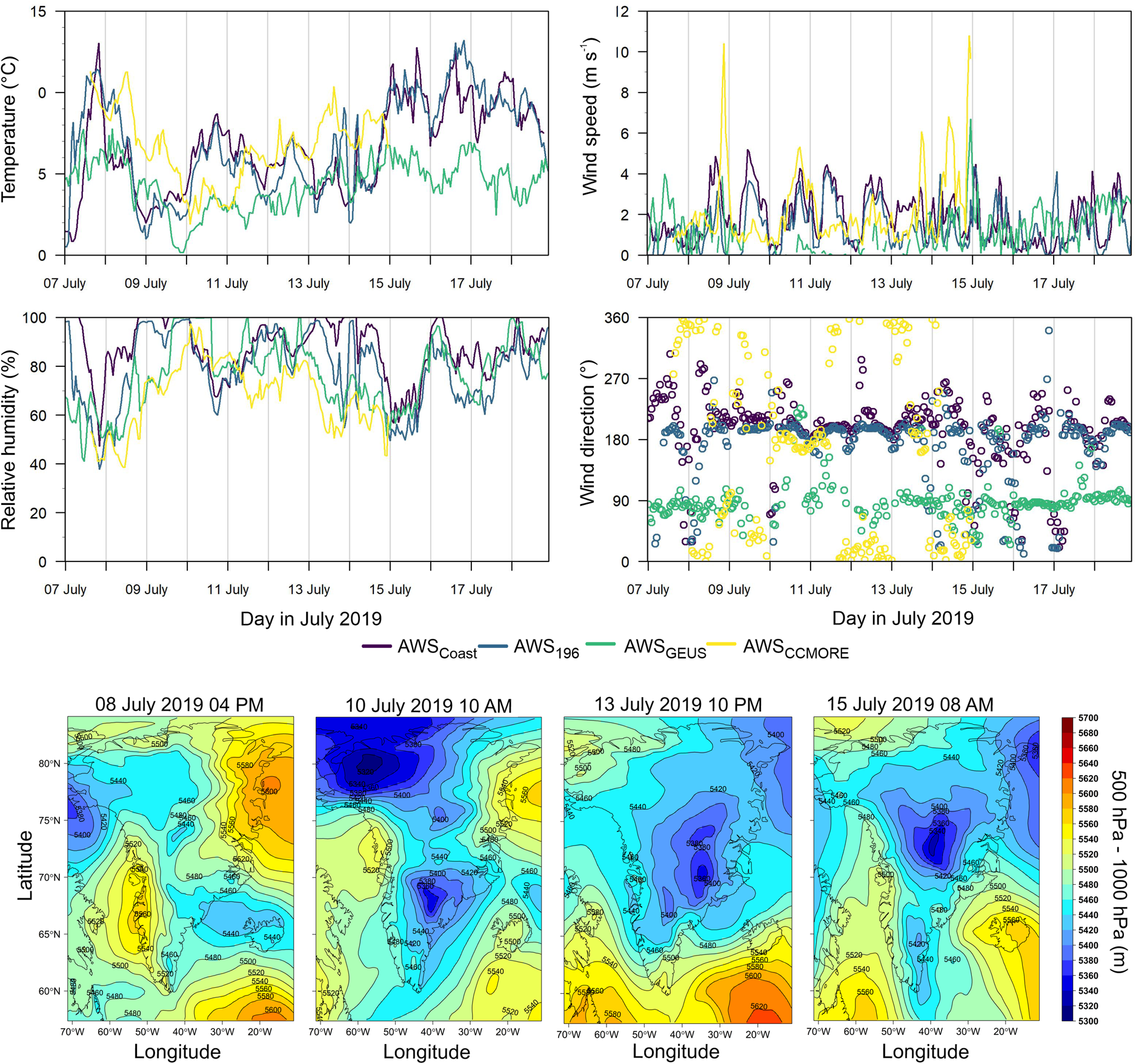
Fig. 2. Top: The time series of atmospheric variables such as air temperature, relative humidity, wind speed and direction of all four AWSs during the field campaign. Bottom: Four points in time during the field campaign showing the atmospheric thickness from ERA5 synoptic weather charts.
What can already be seen visually from the temperature evolution of the AWS in Figure 2 is proven by the analysis of all 113 UAV profiles; temperature inversions occurred frequently in the study area during the study period. Overall, temperature inversions were found in 83% of all UAV profiles. Of these 152 observed inversions, there are 115 EI (76% of all inversions) and 37 SBI (24% of all inversions) (Table 2). However, there are spatial and temporal differences to point out: more EI were identified at locations above gravel or rock (A, B, C, D and H) than SBI, while more SBI than EI were observed at the locations on the glacier (E, F and G) (Fig. 1). In Figures 3 and 4 we see the difference between the interpolated temperature and humidity profiles and the average value of temperature or relative humidity measured at AWS$_{\rm {COAST}}$ during the transect acquisition.
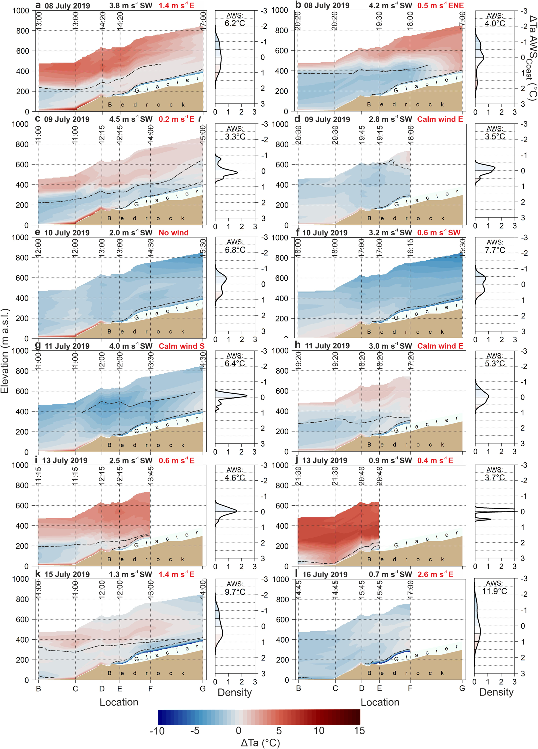
Fig. 3. Difference between the interpolated temperature (Ta) transect and the average temperature measured at AWS$_{\rm {COAST}}$ during the time period of the transect acquisition. To the right of each transect, the temperature variability (deviation from the mean) of AWS$_{\rm {COAST}}$
 during the transect survey is shown as a density function in the same color code as the transects. Inside this density plot, the mean temperature value measured at AWS$_{\rm {COAST}}$
 is given as a number. Each inset shows the time of the profile acquisition (along the dashed lines above the locations), above each inset is the date, average wind speed and main wind direction at AWS$_{\rm {COAST}}$
 (black) and AWS$_{\rm {GEUS}}$
 (red, quantitative data wherever available, if not qualitative data from on-site observations were used) during the transect acquisition. The dashed line indicates the approximate location of the major inversion layers detected (Z$_{\rm {Base}}$
 for EI and Z$_{\rm {Top}}$
 for SBI on the glacier). Approximate glacier bed topography from (Yde and others, Reference Yde2014).

Fig. 4. Difference between the interpolated relative humidity (Rh) transect and the average relative humidity measured at AWS$_{\rm {COAST}}$ during the time period of the transect acquisition. To the right of each transect, the relative humidity variability (deviation from the mean) of AWS$_{\rm {COAST}}$
 during the transect survey is shown as a density function in the same color code as the transects. Inside this density plot, the mean relative humidity value measured at AWS$_{\rm {COAST}}$
 is given as a number. Each inset shows the time of the profile acquisition (along the dashed lines above the locations), above each inset is the date, average wind speed and main wind direction at AWS$_{\rm {COAST}}$
 (black) and AWS$_{\rm {GEUS}}$
 (red, quantitative data wherever available, if not qualitative data from on-site observations were used) during the transect acquisition. In each inset, the period for the transect acquisition is given, below which the average wind speed measured during the transect survey at AWS$_{\rm {COAST}}$
 is shown. The dashed line indicates the approximate location of the major inversion layers detected (Z$_{\rm {Base}}$
 for EI and Z$_{\rm {Top}}$
 for SBI on the glacier). Approximate glacier bed topography from (Yde and others, Reference Yde2014).
Table 2. Observed number of acquired vertical temperature profiles based on our UAV-based measurements, temperature inversions for the different inversion types (SBI and EI)
A reoccurring spatial pattern emerges: in most transects, the near-surface temperature of the locations above the gravel or rock surface types (B, C, D) is higher and the relative humidity is lower compared to AWS$_{\rm {COAST}}$ , with the lowest temperature and relative humidity difference observed at the location B (closest to the ocean) and the highest at the location at C (e.g. Figs 3 and 4 a, c, e). From location C to D, the near-surface temperature decreases slightly, but is still higher than that of AWS$_{\rm {COAST}}$
 . In all transects, the near-surface temperature above the Mittivakkat Gletsjer (location E to G) is lower than the AWS$_{\rm {COAST}}$
 . In most transects, we also see a drier air layer above the glacier surface compared to AWS$_{\rm {COAST}}$
 and the air above. These typical vertical temperature and relative humidity distributions are particularly pronounced in the transects surveyed between late morning and early afternoon (e.g. Figs 3 and 4 a, c, e, i).
Another feature observed in most transects is a cool and moist near-surface air layer and a warmer and drier one above (Figs 3 and 4a–d, h–k). The thickness of this cooler and humid layer varies between transects, e.g. the layer at location B was ~380 m thick on 8 July 2019 (Figs 3 and 4b) while it reached a lower thickness of ~60 m at the same location on 13 July 2019 (Figs 3 and 4j), but has its greatest extent between locations B and C in all transects, further inland the extent decreases. In the area where the cooler air layer borders on the warmer air layer above, a layer with a higher moisture content (~100% relative humidity) than the ambient air can be seen in some transects (Figs 3 and 4 b, c, g).
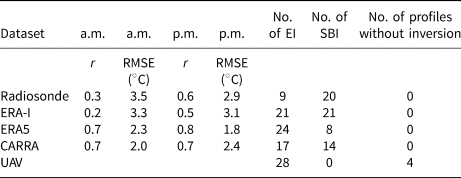
To investigate the differences between the temperature profiles of the UAV measurements and those of the radiosonde and reanalysis data, 21 UAV temperature profiles collected at location A at 10 a.m. or 10 p.m. were compared with the corresponding radiosonde and reanalysis (ERA-I, ERA5 and CARRA) profiles. Table 3 shows the calculated Pearson correlation coefficient and RMSE between the morning (10 a.m.) and evening (10 p.m.) UAV measurements and the radiosonde and reanalysis profiles, respectively. Evidently, ERA5 and CARRA profiles show better agreement with the UAV profiles than the radiosonde and ERA-I profiles. When comparing the morning and evening conditions, it is apparent that the evening profiles generally have a higher agreement. The highest agreement in terms of inversion statistics was found between the UAV and ERA5 (Table 3). Compared to the radiosonde, ERA-I and CARRA profiles, which had a high number of SBI (14–21) and few EI (9–21), the UAV and the ERA5 profiles had a high number of EI (24–28) and a low number of SBI (0–8). Figure 5 shows Δtemperature between the profiles of the datasets under evaluation and those of the UAV (UAV minus radiosonde, ERA-I, ERA5, CARRA). The upper row shows the morning profiles (10 a.m.) and the lower row the evening profiles (10 p.m.). The radiosonde and ERA-I profiles (Figs 5a–d) have the largest mean differences (thick line) compared to ERA5 and CARRA profiles (Fig. 5e–h) near the surface.

Fig. 5. ΔTemperature (ΔTa) of the profiles between UAV and the radiosonde (a, b), ERA-I (c, d), ERA5 (e, f), and CARRA (g, h) profiles for all 10 a.m. (blue) and 10 p.m. (red) profiles. The thicker line (blue for a.m. and red for p.m.) shows the mean Δtemperature. A positive Δtemperature means that UAV temperature is higher than the corresponding dataset. The more transparent color shows the range between minimum and maximum deviation. In the upper right area of the figures the RMSE and the mean difference (MD) are shown.
Table 3. RMSE and the Pearson correlation coefficient between UAV and radiosonde and reanalysis temperature profiles
To explore possible effects of the atmospheric structure on glacier melt, the measured ablation values between 8 July 2019 and 15 July 2019 are shown as ablation per day (color-coded sections in the bars) and mean ablation per day (line) and altitude for the ablation stakes M01, M02, M03, M04 in Figure 6. This figure shows that M03 and M02 have the same ablation of −45 mm w.e. on 9 July 2019 and a slightly higher ablation compared to the lower ablation stake M01 (−36 mm w.e.) and the higher ablation stake M04 (−0.9 mm w.e.). On the following day, M03 shows the highest ablation of −81 mm w.e. compared to all other ablation stakes. The highest mean ablation per day (Fig. 6) was measured at the lowest ablation stake M01 with −51.4 mm w.e. and the lowest with −27.6 mm w.e. at the highest ablation stake M04. The ablation stakes M02 and M03 show an equal mean ablation of −38.5 mm w.e. per day despite a 65 m elevation difference.

Fig. 6. Daily ablation as bars, the entire bar represents the cumulative ablation of the respective ablation stake and the colored areas in the bar represent the ablation that occurred on the respective day. Mean ablation per day and per ablation stake (M01–M04) between 8 and 15 July 2019 is shown as black symbols connected with a line.
6 Discussion
Although this study covers only a short time period, the frequency of temperature inversions found in this study (83%) compares well with the values of similar studies in this region (Mernild and Liston, Reference Mernild and Liston2010; Gilson and others, Reference Gilson, Jiskoot, Cassano and Nielsen2018a). However, with the nature of the presented study as a 2 weeks measurement campaign we can not state that the frequency remains unchanged on the long term. (Semi-)autonomous UAVs (Meteomatics, 2022) or repeated campaigns can shed light on this and should be performed. EI are more common than SBI, which is consistent with other studies (Serreze and others, Reference Serreze, Kahl and Schnell1992; Gilson and others, Reference Gilson, Jiskoot, Cassano and Nielsen2018a). One reason for the high number of EIs compared to SBIs is that there can be multiple EIs in one vertical profile. Another reason could be due to the mesoscale thermal circulation that generally forms during the day in summer over the glacier (Shaw and others, Reference Shaw2017) and near the coast (Miller and others, Reference Miller, Keim, Talbot and Mao2003). In the afternoon, when the temperature contrast between land and sea is largest, the sea breeze is strongly developed, bringing cold and moist air from the sea inland. This cooler and denser air moves below warmer air. In addition to that, valley and slope winds develop, which can cause a valley breeze blowing uphill during the day. Thermal differences between the cold glacier surface and the warmer surrounding air lead to the formation of a shallow katabatic flow (Oerlemans and Grisogono, Reference Oerlemans and Grisogono2002; Ayala and others, Reference Ayala, Pellicciotti and Shea2015). In this case, cooler air is transported down the glacier. The greater the thermal gradient between the surface of the glacier (0$^\circ$ C) and the warm ambient air, the more pronounced the katabatic wind and the stronger the SBI over the glacier surface will become (Oerlemans and Grisogono, Reference Oerlemans and Grisogono2002). For this reason, we observe the highest wind speeds at AWS$_{\rm {GEUS}}$
 on 8, 15 and 16 July 2019 (Figs 2 and 3a, k, l). In particular, on 16 July 2019, the air temperature in the study area was high and the katabatic wind was strong (Figs 2 and 3). As a result, the katabatic flow reached to location D near the terminus and lifted the warmer air layer there, leading to the formation of an EI (Fig. 3 l). Spatial differences in the occurrence of inversion type frequency observed in this study can be explained by different surface types and environmental conditions. Near-surface lapse rates above gravel or rock (locations A, B, C, D, H) are mainly controlled by the surface incident solar radiation. On sunny and clear days, these surfaces warm up and transfer sensible heat to the layers of air above them, leading to a decrease in temperature higher up (Nilsson and others, Reference Nilsson, Rannik, Kumala, Buzorius and O'dowd2020). Therefore, in most of the transects shown in Figures 3 and 4, we see a warm and dry air layer located directly above these surfaces. This air layer is particularly visible at location C, due to its distance from the open water and its sheltered location at the end of the Mittivakkat valley. The warm and dry layer of air near the surface is particularly visible in the transects in the late morning to early afternoon (Figs 3 and 4 a, c, e, g, i) around the time of maximum solar radiation and thus warms the surface. However, the SBIs, which we rarely observed over these surfaces during the field campaign, form when long-wave radiation emitted by the surface exceeds the short-wave radiation reaching the surface. While the lower atmospheric temperature profile is mainly governed by the surface, the intensity of the previously mentioned mesoscale thermal circulation systems, synoptic-scale events and distance from the ocean and valley determine the stratification above. In most transects (Figs 3 and 4 a, b, c, h, i), a cooler and moister air layer is below a warmer and drier one, creating a stable stratification. The depth and extent of the cold, moist layer depend on the strength of the mesoscale thermal circulation systems and synoptic-scale events, which can impact turbulence. The cooler layer is thicker and extends further inland on windier days (e.g. Figs 3 and 4 c) and is thinner and does not reach very far on days with lower wind speeds near the coast (e.g. Figs 3 and 4j). This interaction also affects the inversion characteristics: when the cooler layer is deep and extends far inland, the inversion base is also higher (e.g. Figs 3 and 4b). We can see from the interpolated transects and Figure 2 that this process was observed almost daily in varying intensity and thus it led to the frequent formation of EI in the near-shore area (location A, B, C and D). A higher number of SBI was found at the locations on the glacier (E, F and G) compared to ice-free locations (Table 2). In all transects of Figures 3 and 4 we see a cool and dry air layer directly above the glacier below a warmer slightly more humid air layer. During the melt season, energy is advected from the air layer above the glacier for surface melt which leads to a cooling of the air in contact with the surface. Therefore, SBIs are present in all profiles above the glacier. Other studies have also observed increased numbers of SBI over snow and ice surfaces during the melt season (Miller and others, Reference Miller2013; Ayala and others, Reference Ayala, Pellicciotti and Shea2015; Palo and others, Reference Palo, Vihma, Jaagus and Jakobson2017; Gilson and others, Reference Gilson, Jiskoot, Cassano and Nielsen2018a; Shahi and others, Reference Shahi, Abermann, Heinrich, Prinz and Schöner2020). With the distance from the sea and valley, the influence of the sea and valley breezes decreases along with the frequency of EI. Sixteen percent of the profiles contain no temperature inversions. These profiles were collected mainly between 9 July 2019 evening and 11 July 2019 noon (Figs 3d–g), a period characterized by winds from southwest. This wind is similar in strength (~4 m s−1) at all AWSs except AWS$_{\rm {GEUS}}$
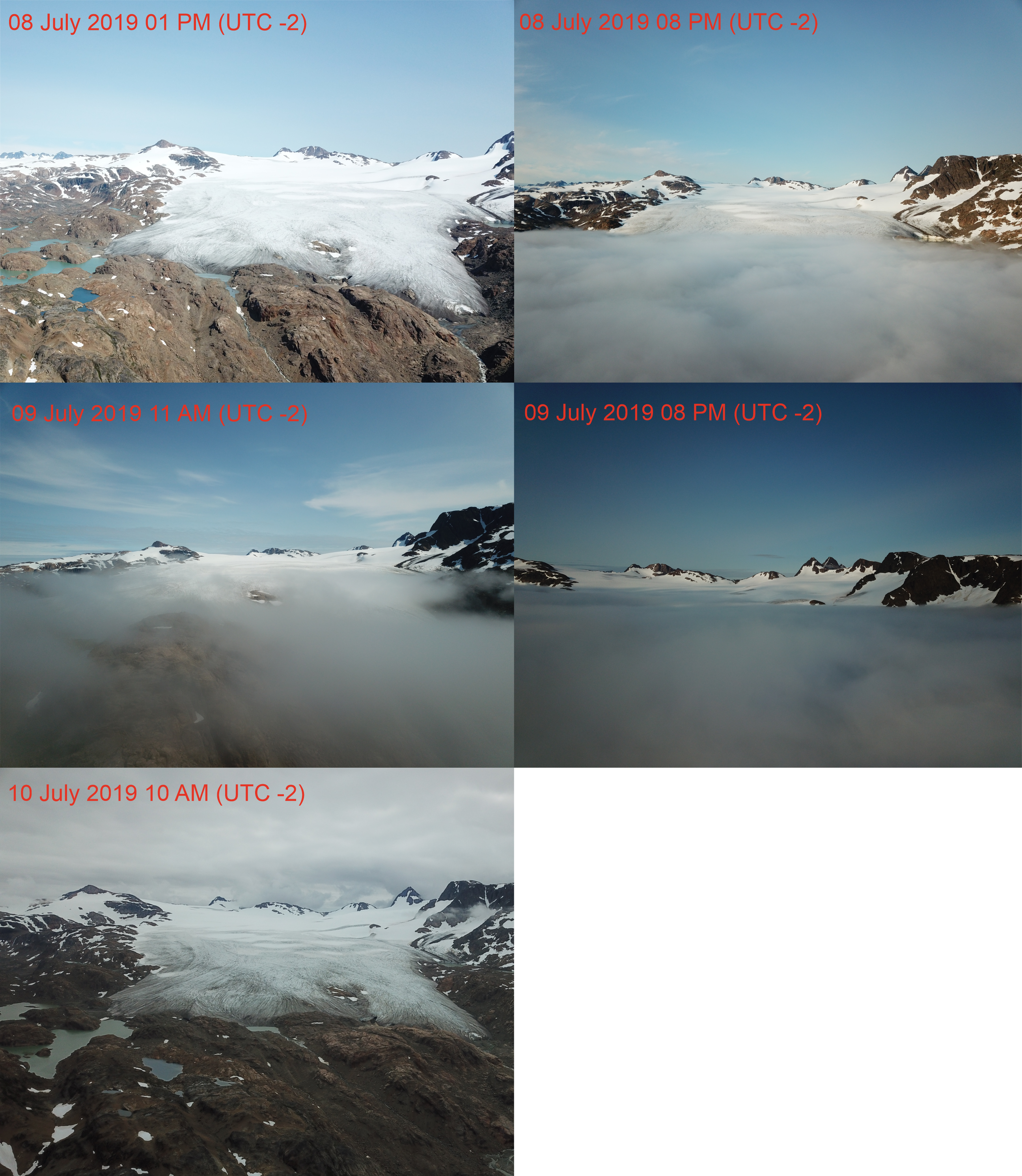
 , where wind speeds do not exceed 1 m s−1. This resulted in a well-mixed atmosphere and prevented the development of inversions. The surface–atmosphere interaction described here and the resulting atmospheric patterns we can observe in the transects improve our understanding of processes that cause the formation and characteristics of inversions. Furthermore, the transects have shown how dynamic the valley atmosphere is both in space and time. Surface types, circulation patterns (e.g. sea breeze) and elevation have an impact on atmospheric stratification and climatic conditions along the valley and glacier. The low spatial and temporal resolution of the radiosonde and reanalysis data do not resolve this complexity as we show by the comparison between the 21 UAVs and 21 radiosondes, ERA-I, ERA5 and CARRA temperature profiles. Reanalysis data are interpolated onto regular grids with coarse spatial resolution, limiting the resolution of complex processes or topography near the surface. As a result, small-scale changes and processes as shown and described in the transects cannot be resolved and represented by the reanalysis data evaluated here. The situation is similar to the radiosonde temperature profiles, which have an even lower spatial coverage and vertical as well as temporal resolution compared to the reanalysis data. These characteristics also affect the inversion statistics. The coarse vertical resolution of radiosonde and ERA-I precludes a realistic representation of thin inversion layers. Therefore, many EI became part of a thick SBI and separate EI layers were often counted as one. The higher agreement of temperature profiles and inversion statistics between the UAV and ERA5 profiles could be due to improvements in the physical parameterization schemes, higher horizontal resolution and the inclusion of more vertical levels leading to a more realistic representation of the Arctic planetary boundary layer. This improved representation of the lower troposphere in the ERA5 data has also been observed in other studies (Graham and others, Reference Graham, Hudson and Maturilli2019; Tetzner and others, Reference Tetzner, Thomas and Allen2019; Palarz and others, Reference Palarz, Luterbacher, Ustrnul, Xoplaki and Celiński-Mysław2020). Spatial heterogeneity in horizontal and vertical temperature, humidity and cloud conditions along the transect affects the spatial variations in snow and glacier melt rates (Mernild and Liston, Reference Mernild and Liston2010; Mernild and others, Reference Mernild, Beckerman, Knudsen, Hasholt and Yde2018). The observed higher ablation at M02 and M03 compared to M01 on 9 July 2019 is associated with a fog layer below the measured inversion layer (210 m a.s.l. at location B, Figs 3 and 4 b, c: Fig. 6). In the afternoon of 8 July 2019, a layer of advection fog formed below 200 m a.s.l., which began to rise around noon on 9 July 2019 to ~300 m a.s.l. (Fig. S2). This is a common type of fog along the Greenland coast in summer (Cappelen, Reference Cappelen2015; Gilson and others, Reference Gilson, Jiskoot, Cassano and Nielsen2018a). Related to the interplay between cool air over the ocean and condensation fog expands inland where it is covered by warmer and drier air (Mernild and others, Reference Mernild, Hansen, Jakobsen and Hasholt2008; Cappelen, Reference Cappelen2015; Gilson and others, Reference Gilson, Jiskoot, Cassano and Nielsen2018a). This situation considerably affects the surface energy budget. The high reflectivity of fog reduces the amount of radiation arriving at the surface, while longwave radiation increases. The net effect usually depends on the droplet size, liquid water path, solar zenith angle and surface albedo (Gilson and others, Reference Gilson, Jiskoot, Cassano and Nielsen2018a). On 9 July 2019 the fog and the cooler air layer beneath the inversion may have led to cooler temperature and lower solar radiation at M01, while the ablation stakes at higher elevations were exposed to higher amounts of solar radiation, inverting vertical ablation gradients (Figs 3 and 4b, c). The same effect could be the reason for the increased melt at M03 compared to M02 and M01 measured on 10 July 2019. Between the 8 July 2019 late afternoon and 9 July 2019 evening, M01 and M02 were most of the time below the fog line (first M01, later M02) in the cooler layer under the temperature inversion, while M03 was most of the time above the fog layer in the warmer region exposed to stronger solar incident radiation. On these days (8 July 2019 late afternoon and 9 July 2019) high wind speeds were observed from the south and southwest (Fig. 2). This cold and moist air from the sea favored the fog formation below the warmer inversion layer. Based on this ablation behaviour, we find a non-linear vertical ablation gradient. Such a non-linear vertical ablation gradient at the lower part of the Mittivakkat Gletsjer was also observed by Knudsen and Hasholt (Reference Knudsen and Hasholt2008). In this study, they summarized the annual mass balances of the glacier for the period 1995–06. The vertical mass-balance gradients shown in this study are non-linear in almost all cases. Troxler and others (Reference Troxler2020) made a similar observation. They investigated the spatial patterns of near-surface air temperature (from 1 to 3 m) over McCall Glacier in Alaska during the ablation period. According to their study, linear lapse rates are inadequate for describing the spatial distribution of near-surface air temperature above the glacier. As a result, glacier melt may be affected. The influence of temperature inversions on glacier melt has been investigated in other studies. A comparison from Hasholt and others (Reference Hasholt, van As and Knudsen2016) between historical ablation measurements at the terminus of Mittivakkat Gletsjer from 1933 (one of the warmest East Greenland summers of the 20th century) with more recent measurements (1996–12) shows that the ablation rates were higher at the terminus in the more recent period than in the historical measurements. Hasholt and others (Reference Hasholt, van As and Knudsen2016) explain this observation by a decrease in surface albedo and the retreat of the Mittivakkat Gletsjer from the cold maritime layer into the warmer inversion layer. Furthermore, Mernild and others (Reference Mernild, Beckerman, Knudsen, Hasholt and Yde2018) investigated the spatio-temporal variability of glacier mass balance on the Mittivakkat Gletsjer. They explained the observed mass-balance variability in the lower part of the Mittivakkat Gletsjer with changes in the duration of the snow cover and the frequent occurrence of temperature inversions in this area. This indicates that the aforementioned total ablation patterns observed on a small temporal scale (e.g. day) are also relevant on a large temporal scale (e.g. season). Hulth and others (Reference Hulth, Rolstad, Trondsen and Rødby2010) found that sustained temperature inversions on Jan Mayen lead to an ablation profile on Sørbreen in which melt does not generally decrease with increasing height. Chutko and others (Reference Chutko, Lamoureux and Shea2009) suggest the increased occurrence of temperature inversions since the late 1980s at Resolute in the Canadian Arctic as an important meteorological mechanism for the increased glacier melt since the late 1980s. Furthermore, Mernild and Liston (Reference Mernild and Liston2010) showed that a realistic representation of temperature inversions properties such as height, thickness and strength in models is essential for accurate snow and glacier ice melt and glacier mass-balance simulations along Arctic coastal landscapes. Especially when we consider that under a changing climate, different and complex patterns of ablation rates can occur locally on glacier surfaces. The results of this study show that the high spatial and temporal resolution of the UAV data can reveal a realistic picture of the high variability of the complex valley atmosphere. Especially, multi-UAV missions, and thus simultaneous atmospheric profiling, allow the state of the atmosphere to be recorded over different surface types or along a predefined transect in a time-efficient manner. While we show the vertical structure's characteristics on a campaign basis during summer 2019, this work should be expanded and implemented into long-term monitoring strategies in order to assess climatological changes.
7 Conclusion
The study shows that the complexity of the Arctic planetary boundary layer during summer can to a large degree be explained by different surface types, local circulation patterns and advection of cold/warm air. This complexity and variability is not captured by the radiosonde and reanalysis data used in this study. We argue that the missing information of the stratification comes from processes inappropriately captured by model physics, deficiencies in assimilation data and low vertical and horizontal resolution. While this missing part of atmosphere patterns in reanalysis is less relevant for studies on Greenland Ice Sheet (due to much less spatially variable surface properties) it becomes highly relevant for the studies of near-coastal environments. We show that UAVs proof to be useful platforms to perform high spatial and temporal resolution measurements of the lower atmosphere. In particular, small-scale processes and changes (e.g.atmospheric stratification patterns leading to complex ablation rates on glacier surfaces) can be well captured by UAV measurements. This information is needed to accurately estimate the effects of climate change (e.g. glacier mass loss, sea-level rise, permafrost thaw depth). Compared to radiosonde or reanalysis data, however, the achievable altitude is lower and the implementation is more complex. Nevertheless, UAV measurements could serve as a complementary data source, especially to improve vertical, temporal and spatial resolution on a campaign basis. This could lead to more accurate observations and research results from studies on the state of the lower atmosphere, as shown in the study by Jonassen and others (Reference Jonassen2015). In addition, technological advances in UAV and sensor technology are expected to address some of the limitations and open up new opportunities in the field of atmospheric research in the future.
Supplementary material
The supplementary material for this article can be found at https://doi.org/10.1017/jog.2022.120
Data
The data used for this study will be made available upon request. Please send all requests to iris.hansche@uni-graz.at.
Acknowledgements
We sincerely thank the EU Horizon 2020 project INTERACT for the funding of the fieldwork and for the use of the Sermilik research station (grant agreement No 730938). Moreover, we thank all data providers. ERA-I, ERA5 and CARRA were produced by ECMWF. Observational data were provided by the University of Copenhagen, University of Graz, the Danish Meteorological Institute and by PROMICE (operated by the Geological Survey of Denmark and Greenland). Thanks to Lars Anker for logistical support. We would also like to express our deep gratitude to the editor, Hester Jiskoot, Alexander Groos and one anonymous reviewer for their valuable time and for their constructive comments and suggestions. The University of Graz is acknowledged for funding the article publication.


 Open access