


1. Introduction
1.1. Overview
Radar-sounding data on the nature of the reflection from the sub-ice interface are essential for understanding the distribution and flow of water in the subglacial environment (Reference Gudmandsen and WaitGudmandsen, 1971; Reference Jacobel and AndersonJacobel and Anderson, 1987; Reference Peters, Blankenship and MorsePeters and others, 2005, Reference Peters, Blankenship, Carter, Kempf, Young and Holt2007; Reference Carter, Blankenship, Peters, Young, Holt and MorseCarter and others, 2007; Reference Matsuoka, Thorsteinsson, Björnsson and WaddingtonMatsuoka and others, 2007). The reflection coefficient from this interface is subject to a considerable degree of uncertainty due to dielectric loss in the overlying ice column. Dielectric attenuation, a function of the electrical conductivity of the ice, varies roughly linearly with chemistry and exponentially with temperature (Reference Corr, Moore and NichollsCorr and others, 1993; Reference MacGregor, Winebrenner, Conway, Matsuoka, Mayewski and ClowMacGregor and others, 2007). The non-linear temperature dependence of the dielectric-attenuation term becomes especially significant for ice near the pressure-melting point (e.g. near subglacial lakes and waterways). Increasing the accuracy of temperature models of the overlying ice will greatly improve the characterization of the subglacial interface using radar.
An improved model for temperature and strain can also constrain basal melt. The current models for basal meltwater production in the East Antarctic interior are either limited to a few discrete points (Reference Bell, Studinger, Tikku, Clarke, Gutner and MeertensBell and others, 2002; Reference Tikku, Bell, Studinger, Clarke, Tabacco and FerraccioliTikku and others, 2005) or rely on a broad order-of-magnitude assumption of 1 mm a−1 (Reference Evatt, Fowler, Clark and HultonEvatt and others, 2006; Reference Wingham, Siegert, Shepherd and MuirWingham and others, 2006). Even the best temperature models to date are still limited by poor spatial resolution of geothermal flux and limited boundary conditions for vertical advection (Reference JohnsonJohnson, 2002). Models based on these calculations may predict basal melting where none is present, and fail to resolve important subglacial geothermal anomalies critical to understanding the flow of the ice sheet (Reference Blankenship, Alley and BindschadlerBlankenship and others, 2001). Accurate quantification of water production in lake districts near ice divides is the first step in understanding how interior subglacial water reaches the onset of fast glacier flow (Reference BellBell, 2008).
Radar-sounding profiles often contain internal reflections that correspond to layers of constant age (Reference SiegertSiegert, 1999). These layers are useful for calculating strain, inferring past surface accumulation and estimating basal melt, all of which significantly affect calculation of ice temperature and basal water production. Recent work with dated internal layers has been used to identify geothermal anomalies, calculate accumulation history and model ice temperature as a function of depth in northeast Greenland (Reference Fahnestock, Abdalati, Joughin, Brozena and GogineniFahnestock and others, 2001; Reference Dahl-Jensen, Gundestrup, Gogineni and MillerDahl-Jensen and others, 2003; Reference Buchardt and Dahl-JensenBuchardt and Dahl-Jensen, 2007).
If the basal melt rate for an entire basin is known, then it is possible to produce a subglacial water budget. Furthermore, estimation of englacial temperatures is required for calculating dielectric attenuation and consequent basal radar reflectivity (Reference Gudmandsen and WaitGudmandsen, 1971; Reference Corr, Moore and NichollsCorr and others, 1993; Reference MacGregor, Winebrenner, Conway, Matsuoka, Mayewski and ClowMacGregor and others, 2007). Using this relationship it is possible to verify a coupled model for temperature and water distribution with the basal reflectivity. Here we use internal layering to estimate strain history, which is then used to construct a temperature model for the ice. Using the modeled temperature of the overlying ice, we calculate dielectric loss and the consequent basal reflection coefficients. In this process we also obtain useful information regarding accumulation history, basal melt and geothermal flux, all of which aid our understanding of the response of the ice to long-term climate change (Reference Carter, Blankenship, Peters, Young, Holt and MorseCarter and others, 2007, Reference Carter, Blankenship, Young, Peters, Holt and Siegert2009; Reference Peters, Blankenship, Carter, Kempf, Young and HoltPeters and others, 2007). We apply this self-consistent method to the Dome C region, East Antarctica, where there exists a relative abundance of radar-sounding data containing continuous internal layers (Reference Siegert, Eyers and TabaccoSiegert and others, 2001) over ten subglacial lakes, three of which have a surface area larger than 100 km2 (Reference Siegert, Carter, Tabacco, Popov and BlankenshipSiegert and others, 2005; Fig. 1) and a dated ice core (EPICA Community Members, 2004).

Fig. 1. (a) Ice surface elevation (m) with moderate-resolution imaging spectroradiometer (MODIS) imagery superimposed for the Dome C area (http://nsidc.org/data/nsidc-0280.html; http://nsidc.org/data/nsidc-0304.html). The coverage of the SOAR/UTIG/SOAR dataset in this area is dense and captures the uppermost part of the Frost and Mulloch Glacier catchments. (b) Ice basal topography (m) from UTIG/SOAR airborne radar dataset with terrain classifications (from Reference Tabacco, Cianfarra, Forieri, Salvini and ZirizzottiTabacco and others, 2006). (c) Map showing location of study in the context of major glacier catchments (Reference Bamber, Vaughan and JoughinBamber and others, 2000) and balance velocities (Reference Le Brocq, Payne and SiegertLe Brocq and others, 2006).
1.2. Dome C: a natural laboratory at the headwaters of two dynamic basins
This study includes 3000 km of radar-sounding data collected by the University of Texas Institute for Geophysics/Support Office for Aerogeophysical Research (UTIG/SOAR) from the area immediately north of Dome C. These data form a rectangular grid approximately 130 km × 150 km (Fig. 1). The unusually high concentration of subglacial lakes in this area was first observed during UK Scott Polar Research Institute/US National Science Foundation/Technical University of Denmark (SPRI/NSF/TUD) surveys during the 1970s (Reference Oswald and RobinOswald and Robin, 1973; Reference Siegert, Dowdeswell, Gorman and McIntyreSiegert and others, 1996, Reference Siegert, Eyers and Tabacco2001, Reference Siegert, Carter, Tabacco, Popov and Blankenship2005) and subsequently confirmed by an Italian survey of the same region (Reference Rémy, Testut, Legrésy, Forieri, Bianchi and TabaccoRémy and others, 2003; Fig. 1) and the UTIG/SOAR data (Reference Carter, Blankenship, Peters, Young, Holt and MorseCarter and others, 2007; Fig. 2). The authors of these studies noted three major characteristics of the ice and bedrock topography that favor the storage of subglacial water in this area: (1) the ice surface slope (and thus the regional hydraulic gradient) is exceptionally low (Fig. 1); (2) the relatively thick ice cover insulates the bed from cold surface temperatures; and (3) the rugged bedrock relief contains a number of hollows that can trap water (Reference Siegert, Carter, Tabacco, Popov and BlankenshipSiegert and others, 2005; Fig. 1).
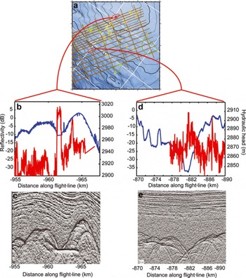
Fig. 2. Hydraulic potential (blue) and reflectivity (red) over (b, c) a lake on the Concordia Ridge and (d, e) a narrow valley in the Belgica Subglacial Highlands. High reflections above −5 dB are found in the relative minima of the hydraulic head. Note that although the lake appears to extend below a diffraction hyperbola, the hyperbola is still picked as the bed to maintain reproducibility with respect to our ice-thickness interpretation algorithm. (a) shows locations of (b–e).
The three largest subglacial lakes in the study area are Concordia, Vincennes and Horseshoe, the first two occupying basins of the same name. A preliminary analysis of the radar returns (Reference Carter, Blankenship, Peters, Young, Holt and MorseCarter and others, 2007), which used one-dimensional steady-state englacial temperature models, showed that all of these major lakes exhibit bright specular reflections that are brighter than the reflections from surrounding areas and they were termed ‘definite lakes’. A second class of lakes, while brighter than the surroundings, is not of consistent brightness across the interface. These ‘fuzzy lakes’ are interpreted as shallow features, possibly ‘swamps’. However, in some cases, simple englacial temperature models present contradictory results. Some subglacial lakes exhibit specular reflections nearly 10 dB lower than that expected for an ice–water interface and are termed ‘dim lakes’ by Reference Carter, Blankenship, Peters, Young, Holt and MorseCarter and others (2007). In at least one of these cases, simple temperature models are not consistent with the existence of liquid water at the base of the ice (Reference Siegert, Dowdeswell, Gorman and McIntyreSiegert and others, 1996). Reference SiegertSiegert (1999) has identified several subglacial lakes near Dome C in areas where water is not expected without enhanced geothermal flux.
The geology of this region can only be inferred from remote sensing and rock outcrops more than 1000 km away. Reference Forieri, Zuccoli, Bini, Zirizzotti, Rémy and TabaccoForieri and others (2004), studying the radar-derived bedrock morphology, inferred that the subglacial landscape is dominated by extensional horsts and grabens. Although the data coverage east of Concordia Ridge is sparser, Reference Tabacco, Cianfarra, Forieri, Salvini and ZirizzottiTabacco and others (2006) identified a continuing series of parallel ridges and valleys with a wavelength of about 30 km (Fig. 1) and a relief of about 500 m.
More accurate information on geothermal flux could improve our understanding of geologic and tectonic processes in the Dome C area. Geothermal flux for this area has been inferred from two low-resolution continent-wide studies using remotely sensed geophysical data, with values of 45 mW m−2 with an error of ±5 mW m−2 (Reference Shapiro and RitzwollerShapiro and Ritzwoller, 2004) and 50 mW m−2 with an error of ±20 mW m−2 (Reference Fox Maule, Purucker, Olsen and MosegaardFox Maule and others, 2005) indicated. Evidence from the EPICA Dome C ice core indicates a basal temperature at or near the pressure-melting point and a geothermal flux between 40 and 50 mW m−2. Recent thermomechanical models for the ice sheet likewise indicate warm basal temperatures through much of the interior (Reference HuybrechtsHuybrechts, 2002; Reference JohnsonJohnson, 2002; Reference ParreninParrenin and others, 2007). These methods cannot identify localized geothermal flux anomalies smaller than 10 km. Such features may result from high bedrock concentrations of radioactive material, isolated volcanism, enhanced hydrothermal flow associated with tectonic features, or topographic focusing (Reference Blankenship, Bell, Hodge, Brozena, Behrendt and FinnBlankenship and others, 1993, Reference Blankenship, Alley and Bindschadler2001; Reference McLaren, Sandiford and PowellMcLaren and others, 2005; Reference Van der Veen, Leftwich, von Frese, Csatho and LiVan der Veen and others, 2007; Reference DanqueDanque, 2008), all of which could indirectly affect the subglacial water budget.
2. Methods
2.1. A self-consistent technique for obtaining reflectivity and water distribution
Here we use airborne radar data and a dated ice core to obtain accurate reflection coefficients for the sub-ice interface. In this process we identify geothermal anomalies and basal melt, ultimately to compare the locations of basal meltwater production against the areas where it is stored. This analysis consists of four parts illustrated in Figure 3. (1) For every basal echo in the data, we calculate the received echo strength and correct it for geometric losses. (2) For every point in our radargram, we use the internal layer stratigraphy to constrain the vertical strain rate and strain history. (3) We then combine paleotemperature data from the Dome C ice core (EPICA Community Members, 2004), the regionally inferred geothermal flux (Reference Shapiro and RitzwollerShapiro and Ritzwoller, 2004) and our strain history to construct a temperature profile. (4) From the modeled temperature profile and depth-dependent impurity concentration of the ice, we then calculate dielectric loss through the ice column and subtract this loss from the basal echo strengths to obtain the basal reflectivity. This reflectivity value can then verify the presence of subglacial water (Fig. 3).

Fig. 3. Flow chart summarizing our algorithm. The algorithm that produces the melt-rate distribution is also used to create the temperature profile for the dielectric loss correction to the basal reflectivity. The basal reflectivity then verifies the water distribution predicted by the melt-rate model.
Additionally, the strain-rate estimates can be used to estimate paleoaccumulation, and the temperature model can provide an estimate of the basal melt rate. These are useful parameters for understanding the ice-sheet evolution and predicting the distribution of water. Each of the individual parts of this method has been demonstrated as effective for understanding a simple system at a few points, but these have never been combined into one comprehensive algorithm, despite the inherent interrelatedness of subglacial water, radar reflectivity, ice temperature, climate history and ice-flow history.
2.2. Data description
2.2.1. Radar data
The UTIG/SOAR airborne geophysical platform for the 1999–2000 RTZ9 campaign consisted of a radar system, a laser altimeter, a magnetometer and a gravimeter mounted aboard a modified de Havilland Twin Otter aircraft. The radar was operated in pulse mode at 60 MHz carrier frequency with a 250 ns pulse width and a 12.5 kHz pulse repetition frequency. Peak transmitted power was ∼8 kW. The receiver had 4 MHz bandwidth and log-detected the return signals, which were then digitized at a 16 ns sampling interval. Additional stacking of 2048 of these digitized signals resulted in a record about every 10–12 m along track (Reference Blankenship, Alley and BindschadlerBlankenship and others, 2001; Reference Studinger, Bell, Buck, Karner and BlankenshipStudinger and others, 2004; Fig. 2c and e).
2.2.1.1. Ice thickness
The digitized records are displayed on a screen where the user ‘picks’ features of interest across radar records (Reference Blankenship, Alley and BindschadlerBlankenship and others, 2001; Fig. 3). In the event that we observe several possible basal reflections, the first arrival is always selected as the base of the ice. Although this rule allows for consistent reproducible interpretation, in areas of steep topography it may also lead to interpretation of diffraction hyperbolae as bed (Fig. 2). The position of the aircraft at each trace is recorded by an on-board global positioning system (GPS). The height of the aircraft above the ice is measured by a laser altimeter. The depth to each selected feature of interest is calculated from the two-way travel time between that feature and the aircraft using a velocity for radar-wave propagation of 300 and 169 m μs−1 in air and ice, respectively. The UTIG data differ from many other radio-echo sounding datasets in that no firn correction is applied. This is due in part to the fact the RTZ9 corridor covers an extensive region from Dome C on the East Antarctic plateau to Drygalski Glacier on the Ross Sea. Across this region firn compaction rates are known to vary extensively such that the errors in ice thickness introduced by the inaccuracies of a single firn compaction model would likely introduce as much error as no firn compaction model at all. Furthermore, when considering basal hydrology, in particular pressure applied by the overlying ice, the uncorrected radar-derived thickness is a closer estimate of the total mass of overlying material than the firn-corrected ice thickness (Reference PatersonPaterson, 1994). The maximum ice-thickness error associated with neglecting the firn correction is ∼12 m, equivalent to a 1 m error in the hydraulic head at the base of the ice.
2.2.1.2. Tracking and dating internal layers
Internal layers in ice-penetrating radar data can result from density contrasts, ice fabric boundaries or changes in ice chemistry (Reference Fujita and MaeFujita and Mae, 1994). In this study we consider only layers resulting from chemical boundaries, as they represent constant time horizons (isochrones) resulting from the widespread deposition of electrically conductive aerosols from distant volcanic eruptions. Starting parallel to the surface, their deformation with burial is a function of the strain within the ice (Reference SiegertSiegert, 1999). The local mechanics of ice behavior can be inferred from their geometry. Where these layers are visible, smooth and continuous, they can be used to extrapolate an age vs depth relationship from an ice core to the limit of layer continuity, thus allowing strain to be quantified (Reference Morse, Blankenship, Waddington and NeumannMorse and others, 2002; Reference Rippin, Siegert and BamberRippin and others, 2003).
Out of 80 internal layers detected in the UTIG/SOAR airborne radar dataset near Dome C, 11 have been selected based on the two criteria of continuity and brightness (Fig. 4a and b; Table 1). Internal layers are traced in Schlumberger GeoFrame seismic interpretation software. The radar amplitudes are differentiated for interpretation, which highlights flat features. The picking is done manually and attempts to follow prominent continuous peaks and troughs in the amplitude. Dates for these layers over the entire region were determined by assuming the same depth–age scale for the layers across the 20 km gap between the point of data in the UTIG/SOAR archive closest to the Dome C ice core (EPICA Community Members, 2004).

Fig. 4. (a, b) Sample radar-sounding profile collected by UTIG/SOAR (a) near Dome C station and (b) on the southeast shore of Concordia Subglacial Lake. Bottom curve corresponds to the basal reflector. The sub-horizontal stripped pattern in the middle corresponds to internal layering. Colored lines are user-defined interpretations of internal layer positions. Note the layers intersecting the bed in (b). (c, d) Vertical velocity (cm a−1) for the point nearest to (c) Dome C and (d) Concordia Subglacial Lake. (e, f) Actual layer thickness and modeled layer thickness by Equation (7) and paleoaccumulation rates (cm a−1) for (e) Dome C and (f) the southeast shore of Concordia Subglacial Lake.
Table 1. Ages and depths of internal layers used in this study at the point closest to Dome C, using the EDC-3 timescale with uncertainties (Reference ParreninParrenin and others, 2007)

We qualitatively verify the extrapolation of the timescale by tracing layers along one line of Italian radar data that connects both the UTIG/SOAR data and the Dome C core site (section 2.2.2). Both the internal layers and the ice–bedrock interface along this line vary by <50 m vertically (Reference Tabacco, Passerini, Corbelli and GormanTabacco and others, 1998). Further verification of layer ages is accomplished by tracking the 42 ka horizon from Dome C to the Taylor Dome ice-core site and comparing ages. Ages recovered for this horizon at both sites are identical (Reference Morse, Waddington and RasmussenMorse and others, 2007). These methods confirm that the 11 selected horizons are indeed accurately dated isochrones and that the set of layers includes at least two horizons from each glacial cycle between the present and 335 ka (Fig. 4; Table 1). Further verification is accomplished by analyzing the crossover error at the 55 crossover points within the Dome C study area (Table 1).
2.2.2. Supplemental data
The UTIG/SOAR radar data for Dome C are complemented by the EPICA Dome C ice core. Completed in 2004, this provides a record of ice composition dating back to over 800 ka (EPICA Community Members, 2004). From strain modeling, internal layers are dated using the EDC-3 depth–age scale (Reference ParreninParrenin and others, 2007). For our temperature model, we use ice-core deuterium data to infer past temperatures for the entire field. Finally, the high-resolution ion chemistry from this core is used to model dielectric attenuation for the reflectivity calculation.
Modern surface accumulation values are obtained from an assimilated dataset consisting of satellite-derived microwave backscatter measurements of snow accumulation combined with point measurements on the surface (Reference Arthern, Winebrenner and VaughanArthern and others, 2006). The initial estimate for geothermal flux comes from a continent-wide map of heat-flow values published by Reference Shapiro and RitzwollerShapiro and Ritzwoller (2004). The values for this map are produced through an inversion of travel times for Rayleigh and Love waves crossing Antarctica to obtain shear wave velocities with depth with a horizontal resolution of ∼200 km. Geothermal flux for Antarctica is inferred by correlating this velocity structure with that of locations elsewhere where flux has been measured. Additional information on the surface slope, used to estimate horizontal temperature advection, comes from the Ice, Cloud and land Elevation Satellite digital elevation model (ICESat DEM) (Fig. 1).
2.3. An integrated model for calculating basal reflectivity
2.3.1. Vertical strain rate
2.3.1.1. Obtaining vertical velocity from internal layers
The vertical velocity at any given layer is calculated using a central difference technique:
where wn , zn and tn are, respectively, the vertical velocity, height above the bed and age for layer n. This equation applies where there is no basal melt. If accumulation is constant with time, then w(z), which actually corresponds to annual layer thickness, will also be equal to the vertical velocity for that layer. In the Dome C region, however, the accumulation has varied by a factor of two or greater over the course of the last 800 ka (EPICA Community Members, 2004). The w values calculated by Equation (1a) are therefore a product of the vertical velocity and the ratio of accumulation rate at time of deposition relative to the longterm average rate. This discrepancy leads to an unacceptable level of random error in the interpolation and extrapolation of the vertical velocity with depth. This error is addressed by considering the cyclical nature of accumulation variations through time and filtering the raw velocity vs depth relationship to get a smoother monotonic relationship. This smoothing is accomplished by using a triangular filter of the set wn −3−wn +3, giving:
where Wn is the time-averaged vertical velocity. This sample width ensures that the filtered samples cross at least one entire glacial cycle of accumulation at all times. It is this filtered W(z) that is used in all subsequent calculations (Fig. 4c and d).
2.3.1.2. Paleoaccumulation rates
We use the output of the strain model to supply the temperature model with a vertical advection rate. For the modern rate, we use filtered velocity W(z). In order to estimate W(z) in the past, we need the paleoaccumulation rate. We obtain this rate using a variation on the Reference Dansgaard and JohnsenDansgaard and Johnsen (1969) model for vertical strain:
where ![]() refers to the time-averaged steady-state velocity, C
av is the long-term average accumulation rate and ρ is the exponent relating the shear thinning rate of an individual layer to its depth. Over subglacial lakes where ice slides, we expect p to be close to 1 and thus identical to the Reference NyeNye (1963) relation for vertical strain rate. At an ice divide, p = 2. Over subglacial highlands, where a larger percentage of the basal ice is subjected to simple shear, p will be higher. Values of p> 3 may occur in ice overriding a mountain range or in other situations in which the vertical thinning rate is highly non-linear with depth. In such cases, Equation (2a) may be a poor approximation (Reference PatersonPaterson, 1994; Reference ParreninParrenin and others, 2007). In order to obtain p and C
av, we invert our previously determined values for Wn, z and h. The inversion uses Wn
and z values from all layers that are 130 ka or younger to capture an entire glacial cycle. The inversion starts by taking an initial guess of p = 2 (Reference ParreninParrenin and others, 2007) and then calculating the least-squares fit to C
av. The L2 norm between calculated
refers to the time-averaged steady-state velocity, C
av is the long-term average accumulation rate and ρ is the exponent relating the shear thinning rate of an individual layer to its depth. Over subglacial lakes where ice slides, we expect p to be close to 1 and thus identical to the Reference NyeNye (1963) relation for vertical strain rate. At an ice divide, p = 2. Over subglacial highlands, where a larger percentage of the basal ice is subjected to simple shear, p will be higher. Values of p> 3 may occur in ice overriding a mountain range or in other situations in which the vertical thinning rate is highly non-linear with depth. In such cases, Equation (2a) may be a poor approximation (Reference PatersonPaterson, 1994; Reference ParreninParrenin and others, 2007). In order to obtain p and C
av, we invert our previously determined values for Wn, z and h. The inversion uses Wn
and z values from all layers that are 130 ka or younger to capture an entire glacial cycle. The inversion starts by taking an initial guess of p = 2 (Reference ParreninParrenin and others, 2007) and then calculating the least-squares fit to C
av. The L2 norm between calculated ![]() and Wn
is then obtained. The best-fit p value is determined iteratively using Newton’s method. Once the converged value of
and Wn
is then obtained. The best-fit p value is determined iteratively using Newton’s method. Once the converged value of ![]() is obtained, the paleoaccumulation rate is then calculated as:
is obtained, the paleoaccumulation rate is then calculated as:
For the greater Dome C region, the depth to the 130 ka horizon is 45–65% of the total ice thickness (Fig. 5c and d).

Fig. 5. (a, b) Modeled temperature history and (c, d) consequent dielectric profiles for (a, c) Dome C and (b, d) southeast Concordia Subglacial Lake. From 254 to 130 ka the model results are treated as a ‘spinning-up’ phase and therefore not used for final calculations of melt and geothermal flux. The control profile for each dielectric loss plot is based on assuming constant bulk impurity concentration with depth.
2.3.1.3. Basal melt-rate extrapolation
Although the melt rate of basal ice influences the vertical strain rate and position of the internal layers, interpretation of the deepest internal layers is often complicated. For example, the 335 ka horizon intersects the base of the ice near Concordia Subglacial Lake but is found nearly 900 m above the base of the ice in the southeast corner of the survey. Although layers older than 335 ka are found near Dome C and Concordia Trench, continuity problems arise when trying to trace those layers over the escarpment of Concordia Ridge or into the high-melt area of Concordia Subglacial Lake (Reference Tikku, Bell, Studinger, Clarke, Tabacco and FerraccioliTikku and others, 2005). In order to address the apparent absence of deep dated layers we perform the vertical strain-rate extrapolation only in areas where z/h≤0.2. For these areas in which the height of the deepest layers is sufficiently close to the bed, we use a model fitting the deepest six points for Wn and z to the calculated velocity mw , which is simply the vertical velocity at z = 0:
This follows the Nye model for vertical velocity vs depth, although this model is not robust at significant ice divides. mw values less than the uncertainty in the fit (1.5 mm a−1 or ∼5% of the mean accumulation rate) are flagged as irresolvable basal melt (Fig. 5a and b). This value, 1.5 mm a−1, is also approximately equal to the uncertainty in geothermal flux (section 4.1).
2.3.2. Vertical strain, ice-core records and temperature modeling
Previous temperature-modeling efforts in the Dome C region have been limited to Dome C (Reference Masson-DelmotteMasson-Delmotte and others, 2006; Reference ParreninParrenin and others, 2007) or have not incorporated a realistic strain and accumulation history (Reference Tikku, Bell, Studinger, Clarke, Tabacco and FerraccioliTikku and others, 2005). The model described in this paper applies a modified technique first developed for internal layers in northeast Greenland to incorporate the effects of variations in surface temperature and surface accumulation in the current temperature profile (Reference Dahl-Jensen, Gundestrup, Gogineni and MillerDahl-Jensen and others, 2003). Conservation of energy is expressed as:
where T is the temperature, t is time, p ice is the density of ice (917 kg m−3), Cp is the heat capacity of ice (2177.3 J kg−1 K−1), K is the thermal conductivity of ice (W m−1 K−1) and ω is a normalized vertical velocity function (described below), with the Dirichlet boundary condition,
where subscript s refers to conditions at the ice surface. T s is treated as a function of ice surface elevation and time by the formula:
The lapse rate ![]() is 10°C km−1 (Reference PatersonPaterson, 1994; Reference Magand, Frezzotti, Pourchet, Stenni, Genoni and FilyMagand and others, 2004). The temperature record from Dome C,
is 10°C km−1 (Reference PatersonPaterson, 1994; Reference Magand, Frezzotti, Pourchet, Stenni, Genoni and FilyMagand and others, 2004). The temperature record from Dome C, ![]() , is determined from stable-isotope work on the Dome C ice core (EPICA Community Members, 2004). At z = 0, a Cauchy boundary condition is applied:
, is determined from stable-isotope work on the Dome C ice core (EPICA Community Members, 2004). At z = 0, a Cauchy boundary condition is applied:
where G is the geothermal flux. ω(z) is a shape function of the vertical velocity vs depth that has been normalized for the local paleoaccumulation rate:
with c(t) determined using c(z) (Equation (2b)) evaluated for each dated layer and c(0) being the modern accumulation rate. To calculate temperature as a function of depth through time, Equation (4) is solved numerically starting with the steady-state temperature case:

where k is the thermal diffusivity of ice (Reference PatersonPaterson, 1994). The time-step Δt is 100 years, and the vertical step Δz is ∼200 ± 10 m, depending on the exact ice thickness. From this initial state, the model is run with surface temperature continuous from 254 ka to present defined by Equation (5) and the accumulation history c(t) defined by Equation (3) from 130 ka to present. This is to be repeated for the 254–130 ka and the 130 ka to present intervals. If Equation (5) results in a basal temperature above the pressure-melting point T pm, G is modified by the algorithm,
An initial melt rate, mT , is then calculated as:
where L f is the heat of fusion for ice (3.335 × 10⁵ J kg−1). This in turn modifies the velocity function by:
A new temperature profile is then calculated using Equation (3), substituting ω′ for ω. This first iteration of G′, mT and ω′ tends to overestimate melting and produce a basal temperature that is slightly below the pressure-melting point. It is therefore necessary to repeat the iteration until convergence of G′, mT and ω′ is achieved. Two to three iterations are usually sufficient.
The final model (Fig. 5a and b) is a temperature history from 254 ka to the present for ten equally spaced horizons in the ice column (including the ice surface and ice base), the initial melt rate, mT (t), the amount of heat conducted into the ice, G′, and the amount of geothermal heat that goes into melting, G–G′.If the time-averaged mT differs from mw by more than 1.5 mm a−1,the model is repeated with a new geothermal flux defined by
The ultimate result of this modeling is a layer-constrained determination of a modern melt-rate distribution over the entire survey area.
2.3.3. Dielectric attenuation
The attenuation of electromagnetic waves at frequencies near 60 MHz through ice is a function of the ice temperature and ionic chemistry (Reference Gudmandsen and WaitGudmandsen, 1971; Reference Corr, Moore and NichollsCorr and others, 1993). Most of the dielectric-attenuation models that have used these parameters have assumed a constant impurity concentration with depth (Reference Doebbler, Blankenship, Morse, Peters, Clifford, George and StokerDoebbler and others, 2001; Reference Peters, Blankenship and MorsePeters and others, 2005; Reference Carter, Blankenship, Peters, Young, Holt and MorseCarter and others, 2007). Recent work has highlighted the importance of using site-specific values for impurity concentration (i.e. chemistry) (Reference MacGregor, Winebrenner, Conway, Matsuoka, Mayewski and ClowMacGregor and others, 2007). To estimate the spatial variation of the chemistry, it is useful to convert the relationship to chemistry vs age. Assuming that layers are also horizons of constant chemistry (as well as age), we use the layers to extrapolate a depth-dependent impurity-temperature dielectric loss model. All ice below the deepest dated layer is assumed to have the mean chemistry. This extrapolation is justified because the deepest ice is typically the warmest, and the dielectric loss in warmer ice is dominated by the pure ice component (Reference MacGregor, Winebrenner, Conway, Matsuoka, Mayewski and ClowMacGregor and others, 2007).
2.3.3.1. Dome C ionic chemistry
We extrapolate chemistry along the internal layers using EPICA Dome C chemistry data. The long-term record comes from E.W. Wolff (unpublished data) for Na+, Ca2+ and SO4 2− running to nearly the bottom of the ice core with a vertical resolution of about 2.5 m. Partial data for NO3 and Cl extend to 62 ka, or about 30% of the ice thickness, with a vertical resolution of 1 m (Reference RöthlisbergerRöthlisberger and others, 2003). Concentrations of Cl below the 62 ka horizon are extrapolated via a linear correlation with Na. Likewise, concentrations of NO3 are extrapolated for greater depths through correlation with Ca (Reference Wolff, Jones, Bauguitte and SalmonWolff and others, 2008). Each of these ionic concentrations is converted to a relevant concentration through a charge balance (Reference MacGregor, Winebrenner, Conway, Matsuoka, Mayewski and ClowMacGregor and others, 2007):
where ss indicates the sea-salt component and xs indicates the excess above that. We determine [ssSO4] and [xsSO4] using the conservative ion methods, with ion ratios appropriate for Dome C ice obtained from E.W. Wolff (unpublished data).
2.3.3.2. Dielectric loss and basal reflectivity
With the chemistry and temperature calculated for the entire ice column at a vertical resolution of ∼2.5 m, the dielectric attenuation, A, is calculated after Reference Corr, Moore and NichollsCorr and others (1993) as:
M pure is the conductivity of pure ice (4.1 μs m−1), μ H+ and μ Cl− are the molar conductivity of acid and salt ions respectively (3.2 and 0.43 μs m−1 M−1, respectively), E pure, E H+ and E Cl− are the activation energies of pure ice, acid and salt (0.50, 0.20 and 0.19 eV, respectively), b is Boltzmann’s constant (8.6175 eV K−1), T r is the reference temperature of 251 K and a is a constant that relates dielectric attenuation to conductivity in ice (919 dB m S−1). A number of these parameters, in particular M pure, are subject to a considerable degree of uncertainty. For this reason, reflections from Concordia Subglacial Lake were used to calibrate M pure, with the resulting value at the lowest end of reported values (Reference MacGregor, Winebrenner, Conway, Matsuoka, Mayewski and ClowMacGregor and others, 2007; Fig. 5c and d). The dielectric absorption vs depth is then integrated and multiplied by 2 to obtain the total dielectric loss. We use the radar equation (e.g. Reference Peters, Blankenship and MorsePeters and others, 2005) to account for losses in the bed echo strength: the dielectric loss, the geometric-spreading loss, the ice–air transmission loss and respective gains of the antenna and receiver. From this we obtain the final basal reflectivity.
3. Results
3.1. Basal reflectivity
The basal reflectivity shows a consistent reflection coefficient near −5 ± 3 dB across all areas where subglacial water is known or suspected to collect (Fig. 6a and b). Along most local minima in the hydraulic head we likewise find reflection coefficients between −15 and −5 dB, which is consistent with intermittent pools of water or saturated sediments (Reference Gudmandsen and WaitGudmandsen, 1971; Reference Peters, Blankenship and MorsePeters and others, 2005). These reflections are slightly dimmer where the slope in the hydraulic head along the valley floor is greater and water is more likely to channelize. We find very low basal reflectivity throughout most of the Concordia Ridge, the unnamed ridge-and-peak system and the Belgica Subglacial Highlands. The two bright reflectors within these areas are due to one subglacial lake along Concordia Ridge and a deep previously undetected subglacial lake within a narrow canyon in the Belgica Subglacial Highlands (Fig. 2d).

Fig. 6. (a) Hydropotential (m) from UTIG/SOAR airborne radar data and BEDMAP compilation (Reference Lythe and VaughanLythe and others, 2001). (b) Basal reflection coefficients (dB). White contour indicates −10 dB criteria used by Reference Carter, Blankenship, Peters, Young, Holt and MorseCarter and others (2007) for absolute reflectivity. High reflectivity is found along all the major flow paths, although each flow path contains sections of low reflectivity. (c) Basal melt (mm a−1) from the temperature model mT. (d) Basal heat flow (mW m−2) inferred by temperature modeling. The remotely inferred heat-flow values (Reference Shapiro and RitzwollerShapiro and Ritzwoller, 2004; Reference Fox Maule, Purucker, Olsen and MosegaardFox Maule and others, 2005) are sufficient to keep all of the thickest ice at the pressure-melting point. Anomalous heat flow is necessary to explain the melting of basal material in the Vincennes and Concordia basins.
3.2. Vertical strain rate and the highest basal melt rates
We expect the thinning-rate exponent p from our modified Dansgaard and Johnsen formula described by Equation (2) to vary smoothly across the study area. A map of this parameter (Fig. 7) reveals mostly creeping ice around the highlands, with near-sliding conditions associated with Concordia Trench, Concordia Subglacial Lake and the lower part of Vincennes Basin. The one area in which p varies more rapidly is over the Belgica Subglacial Highlands.

Fig. 7. p exponent of thinning rate vs depth from Equation (2). p varies smoothly through the study area except possibly in the Belgica Subglacial Highlands (left side), where the flow is complicated by a series of gorges carved into the tableland.
There are three locations within the study area where basal melt produces an observable drawdown in the internal layers. The first location, on the edge of Concordia Subglacial Lake (Fig. 4b), has a melt rate of ∼4 ± 1 mm a−1, ∼10–20% of the accumulation rate (Fig. 4f). This is one of two locations in the study area where layers are observed intersecting the base of the ice. The upper Vincennes Basin also shows several smaller drawdown anomalies indicating a melt rate of up to 2 ± 1 mm a−1. The third and perhaps most interesting area of concentrated basal melt occurs over the Concordia Ridge subglacial lake, discussed in section 3.1 (Fig. 2c). Melt rates for the remainder of the region are obtained from the temperature model.
3.3. Paleoaccumulation
The inversion for the thinning rate of the upper 130 ka of ice shows a smooth variation in the p parameter throughout the survey area. Accumulation rates over the last 130 ka have varied from 1.5 to 6.0 cm a−1 throughout the study area, with higher accumulation rates occurring toward the grid northeast corner and lower accumulation near the grid south portions of the Belgica Subglacial Highlands and the unnamed ridge and peaks (Fig. 8). The accumulation-rate difference between highest and lowest accumulation values in our study area varies from a factor of 1.5 at the present to 2.5 during the Last Glacial Maximum (41.5 ka) and 2.0 during the Eemian Interglacial (130 ka). After the Eemian Interglacial, the regional mean accumulation rate decreased gradually, remaining at 90% of the Eemian values at 96.5 ka. A much greater drop in accumulation rate is associated with the period 96.5–80.5 ka.

Fig. 8. Paleoaccumulation rates for a full glacial cycle calculated by Equation (2). Gray shading denotes areas for which the local-layer approximation parameter D> 0.5. Black indicates places where D> 1.0.
3.4. Temperature model
The temperature vs depth profile given by the time-varying model (Equation (9)) yields a colder average temperature for the ice column than would result from a steady-state model using modern values for accumulation and surface temperature. This result is expected, as the current interglacial period is relatively warm and the temperature of the deep ice is influenced by the colder climates of the Last Glacial Maximum (Reference PatersonPaterson, 1994). The basal temperatures, however, generally remain unchanged. Approximately 66% of the bed is either at or near the pressure-melting point, with the possible exception of several subglacial peaks and the Belgica Subglacial Highlands. The entire Dome C plateau is at the pressure-melting point. The temperature model indicates that the base of the ice can remain at the pressure-melting point without any enhanced geothermal flux. A few exceptions are found along the upper edge of the Vincennes Basin and the Belgica Subglacial Highlands.
3.4.1. Melt rates based on the temperature model
The temperature-derived basal melt rate (using Equation (9)) is shown in Figure 6c. The initial mT calculation uses the tomographically inferred geothermal flux of Reference Shapiro and RitzwollerShapiro and Ritzwoller (2004). When mw (derived from vertical strain rates) exceeds this initial assumed value for mT by more than 1.5 mm a−1, the geothermal flux is forced such that the final mT should equal mw in these areas. Because areas of low basal melt (<1.5 mm a−1) are also associated with a relatively large separation between the deepest traced layer and the base of the ice, we argue that the temperature model estimates for basal melt are more reliable than vertical strain-rate estimates. In general the temperature model predicts lower basal melt rates than the strain-rate model when the deepest dated internal layer is more than 20% of the ice thickness above the bed. The only exceptions occur in the Concordia Trench. This may be an artifact of the model, or it may reflect the inevitability of basal melt under 4 km thick ice, even with low geothermal flux (Fig. 6c). The temperature model also predicts basal melt in all the deep basins, except for one anomalous basin directly grid west of Concordia Ridge. In general, melt occurs anywhere that ice is thicker than 3500 m.
4. Discussion
4.1. Sources of uncertainty in the combined model
Errors in calculating the reflection coefficient can occur during any part of the process. The ages within the Dome C ice core have an increasing degree of uncertainty with depth. The exact depths of the layers are also uncertain. The parameters for the dielectric loss equation (Equation (15)) are subject to a considerable degree of calibration for each survey area (Reference MacGregor, Winebrenner, Conway, Matsuoka, Mayewski and ClowMacGregor and others, 2007). Moreover the neglect of horizontal temperature advection, and the assumptions of climate cyclicity and a specular basal interface all introduce a degree of uncertainty. Of these sources of error the dielectric coefficients are the easiest to calibrate, as the influence of this parameter is least likely to change for a given system and field area. The remaining sources of error and assumptions must be evaluated on a case-by-case basis.
4.1.1. Age and depth of internal layers
In addition to the previously discussed uncertainties related to dielectric parameters, we also consider uncertainty related to errors in layer interpretation and uncertainty in the original depth–age scale. Additionally, we examine errors related to neglecting two-dimensional strain. For layer depth we use the L2-norm crossover errors. For layer ages, we use the published value of ±6 ka (Reference ParreninParrenin and others, 2007; Table 1).
We evaluate the errors with layer depth and layer age statistically. We run the model 30 times on a subset of the data in which we have added random noise to our layer depths equivalent to our uncertainty. This experiment is then repeated, adding noise to the layer ages in the same fashion as it was added to the layer depths.
We propagate these error bounds for layer age and layer depth to basal reflectivity, basal melt rate, geothermal flux, paleoaccumulation and the strain constant. The mean error for reflectivity is ±3.3 dB, although this uncertainty is not distributed evenly across the study area. For most of the region the error is substantially below this value; however, in the vicinity of mountainous topography, the magnitude of error increases to nearly ±10 dB. This amplification results from the close spacing of the deepest layers in ice overriding prominent topography. Our estimated error for modeled geothermal flux is ±12 mW m−2. The error for basal melt rate derived from the temperature model is ±1.1 mm a−1, which roughly correlates with the total melt rate. Accumulation errors are ±0.3 cm a−1 for the 14 ka horizon and ±1.9 cm a−1 for the 130 ka horizon. This increase is in part proportional to error related to the age of the layer. The p exponent has an error range of ±0.2, generally lower near Dome C and Concordia Subglacial Lake and significantly higher farther away from Dome C, especially in the areas east of Horseshoe Lake.
4.1.2. Influence of topography and horizontal ice motion on strain rate
When calculating paleoaccumulation rates we assume that vertical strain rate can be approximated with a one-dimensional model while ignoring the horizontal propagation of spatial variations in bed topography and accumulation rates. This assumption, also known as the local-layer approximation (LLA), can be tested through a formula presented by Reference Waddington, Neumann, Koutnik, Marshall and MorseWaddington and others (2007). If paleoaccumulation is calculated as
we can use the non-dimensional depth number D calculated by the formula:
where

Generally, if D ≪ 1 the LLA is valid. For u we use the previously stated u srf value of 0.5 m a−1 parallel to the surface slope of the ice (Reference Legrésy, Rignot and TabaccoLegrésy and others, 2000; Reference VittuariVittuari and others, 2004). We therefore modify the path length by specifying t = tn − tn −1. This will result in lower values of D than calculated by Reference Waddington, Neumann, Koutnik, Marshall and MorseWaddington and others (2007). We justify this modification on the basis that: (1) we use the paleoaccumulation rates primarily for the temperature calculation; (2) the present total thickness of ice of a given age is more significant for calculation of the vertical temperature profile than the actual accumulation rate at the time of deposition (Reference Leysinger Vieli, Siegert and PayneLeysinger Vieli and others, 2004); and (3) our paleoaccumulation calculation considers only the time interval from tn to tn −1.
For all age intervals we obtain D values between 0.1 and 0.5, with values below 0.1 found only for the 0.0–14.7 ka interval and then only over Concordia Trench and Vincennes Basin. For most intervals, values >0.5 generally occur only over the Belgica Subglacial Highlands, the unnamed ridgeand-peak system and the steepest sections of Concordia Ridge. For the interval between 96.6 and 129.7 ka, D values >0.5 are more widespread. Using the total age instead of the differential age, D values exceed 0.5 almost everywhere for layers older than 41.5 ka. The decreasing reliability of the LLA with layer age is compensated by the decreasing significance of errors in accumulation rate with age. As there are few measurements of ice-flow direction and velocity in this area at present, and agreement between the direction of the radar profiles in this study and the direction of ice flow is unknown, the LLA may have to serve as a proxy until a more detailed study of paleoaccumulation is conducted for the region (Reference MacGregor, Matsuoka, Koutnik, Waddington, Studinger and WinebrennerMacGregor and others, 2009).
4.1.3. Influence of horizontal ice motion on temperature
To address the influence of horizontal advection, a sensitivity study is conducted in which horizontal advection is included by a redefinition of the surface temperature T′(t,x,y) boundary condition:
The value Δh s(x, y) is determined from an ICESat surface elevation grid (http://nsidc.org/data/nsidc-0304.html), smoothed using a 50 km low-pass filter, and the horizontal velocity components u and v are determined from the maximum values of the interferometric synthetic aperture radar (InSAR) surface velocity work and published GPS results (Reference Legrésy, Rignot and TabaccoLegrésy and others, 2000; Reference VittuariVittuari and others, 2004). For this region, the ice surface velocity is ∼0.5 m a−1. The difference in basal reflectivity calculated using this parameterization for horizontal advection and a parameterization calculated assuming no horizontal advection is <3 dB at all locations, with the strongest influence exerted over the northern Belgica Subglacial Highlands. This is expected since the ice-surface slope throughout the Dome C region is exceptionally low and the surface velocities are likewise <1 m a−1 (Reference Legrésy, Rignot and TabaccoLegrésy and others, 2000; Reference VittuariVittuari and others, 2004; Reference Le Brocq, Payne and SiegertLe Brocq and others, 2006).
4.1.4. Paleotemperatures and impurities
The discussion above describes uncertainty due to adjusting constants within the dielectric-loss equation, a very simply parameterized term for horizontal advection in the temperature model, using a steady-state temperature model and assuming uniform impurities with depth over the study area. However, by far the greatest sensitivity in all the results arises due to paleotemperatures. Here the steady-state model differs from the time-varying model by more than 15 dB in places, especially around Horseshoe Lake and the Dome C plateau. A steady-state temperature model using modern values or values over the glacial cycle simply cannot sufficiently replicate the attenuation in the ice column with reasonable accuracy in any area of complicated ice flow and climate history. These results imply that the ±5–10 dB of error in the calculation of reflection coefficients in these areas is small compared with paleotemperature effects.
A recent study at Siple Dome indicated that variable impurity concentration with depth may give estimates that vary by ±1 dB km−1 compared with those for depth-averaged chemistry (Reference MacGregor, Winebrenner, Conway, Matsuoka, Mayewski and ClowMacGregor and others, 2007). Our own calculations confirm that this effect is indeed on the order of ±1 dB km−1 for our study area. If we assume that ice chemistry is entirely a function of climate, then it is likely that the eight glacial cycles contained in the ice near Dome C effectively average out the chemistry (EPICA Community Members, 2004); nevertheless, incorporating depth-dependent impurities should increase accuracy. As with the Siple Dome study, we found far more uncertainty with the actual dielectric parameters. Our value for M pure was significantly lower than the value used by Reference MacGregor, Winebrenner, Conway, Matsuoka, Mayewski and ClowMacGregor and others (2007). Other measurements for this parameter at frequencies between 0.02 and 9700.00 MHz have varied considerably. It is not immediately clear whether this is due to the radar system or the ice used for measurement. However, given that this parameter is unlikely to vary spatially for a given radar system and field area, calibrating M pure over an interface where the reflection coefficient is known should result in sufficient accuracy. For this reason, relative reflectivity remains relevant in identifying subglacial water (Reference Carter, Blankenship, Peters, Young, Holt and MorseCarter and others, 2007).
4.1.5. Other factors
Although, to date, this study represents the most comprehensive application of radar stratigraphy and reflectivity to the Dome C subglacial lakes and their interaction with the East Antarctic ice sheet, there are still significant parameters that have not been considered that may be important in future research. The temperature model has not dealt with the effect of shear heating on the basal ice. This effect is expected to be small, given the low velocities in the Dome C region, but even this small contribution may make an important difference in areas where ice flows over steep high-amplitude subglacial topography.
The influence of topography on focusing heat flow (Reference Van der Veen, Leftwich, von Frese, Csatho and LiVan der Veen and others, 2007) has also been neglected. As with shear heating, this effect may prove highly significant in the Concordia Trench, the unnamed ridge-and-peak system and the canyons of the Belgica Subglacial Highlands. However, given the amount of basal ice that is at or near the pressure-melting point without enhanced geothermal flux, this effect is not expected to have a major impact on the total melt production. The most significant omission is neglecting ice-sheet surface change over time. Several of the lakes in this study are at saddle points in the hydraulic head surface. A slight surface change could have the effect of diverting a considerable amount of water into another drainage area (Reference CarterCarter, 2008; Reference Wright, Siegert, Le Brocq and GoreWright and others, 2008).
The current version of the temperature–dielectric-loss model used in this study gives reflection coefficients for subglacial water between −5 and 10 dB, frequently in contrast to the theoretical value of −3 dB. Reflection coefficients greater than zero indicate that more energy at the basal interface is coming back than is being transmitted into it, a physically unrealistic situation. This situation is especially prevalent with the smaller subglacial lakes and portions of subglacial lakes immediately adjacent to steep bedrock topography (e.g. Fig. 2). Given that the shoreline areas of all subglacial lakes contain regions where the adjacent bedrock supports some of the weight of the overlying ice, it might be expected that the sub-ice interface is a few meters higher near the shore of the lake than at its center (Reference Ridley, Cudlip and LaxonRidley and others, 1993), resulting in a concave interface. The resulting geometric amplification would be 2–9 dB (Reference Bianchi, Forieri and TabaccoBianchi and others, 2004). Indeed, given the difficulties in locating and identifying smaller subglacial lakes, the topographically enhanced reflections may serve as a valuable indicator of these environments (Reference Carter, Blankenship, Peters, Young, Holt and MorseCarter and others, 2007). This effect, however, cannot explain all of the observed reflections above 0 dB. Despite the advances in determining absolute reflectivity, relative reflectivity and specularity are still critical for detecting known subglacial water (Reference Carter, Blankenship, Peters, Young, Holt and MorseCarter and others, 2007).
4.2. Implications
4.2.1. Developing and verifying subglacial water models with radar-sounding data
Our model for vertical strain and basal melt, when combined with the hydraulic head surface, should predict a rudimentary water distribution. The associated model for englacial temperatures and consequent dielectric loss, when combined with the basal reflection amplitude, can then verify the presence or absence of water in those locations where water is expected to flow and collect. There is an element of non-uniqueness to this process. For example, through a significant reduction in geothermal flux it is possible to significantly reduce basal melting. This would also reduce modeled englacial temperatures and corresponding dielectric loss correction. It is then possible that the reduced water distribution predicted by such a model will match the consequent reduced basal reflectivity. However, some constraints are provided by the initial strain model. In areas where this model indicates melt rates >1.5 mm a−1 we can be more certain about the geothermal flux and rate of water production. In areas where the strain model predicts a lower melt rate, we then know the maximum possible geothermal flux for that location.
Melting has been identified upstream of all locations from which we observe bright reflections. However, areas in which melt is produced do not always have bright basal reflections. In these areas the hydraulic gradient is typically sufficient to prevent ponding, and the thickness of any water sheet is thus limited. Indeed there is a strongly negative correlation between hydraulic gradient and basal reflectivity even in locations where there appears to be a monotonically descending path from areas of high basal melt to known subglacial lakes, such as the area immediately upstream of Subglacial Lake Vincennes (Fig. 6). However, further modeling of the water system is needed to explain fully the basal reflections outside of subglacial lakes (Reference CarterCarter, 2008).
Among the subglacial lakes of all classifications the reflections are remarkably consistent within the prescribed error bounds. One of the most interesting finds of this study is the bright reflection from the subglacial lake on Concordia Ridge. Earlier studies have suggested that this previously discovered lake had a very dim reflection (Reference Carter, Blankenship, Peters, Young, Holt and MorseCarter and others, 2007) and that the relatively thin ice cover over the lake (∼2.5 km) was insufficient to keep the base of the ice at the pressure-melting point given the background geothermal flux of 50 mW m−2 (Reference Dowdeswell and SiegertDowdeswell and Siegert, 1999). Using the technique described in this paper, the ice above this lake is found to be at the pressure-melting point and the reflection coefficient for the lake surface is nearly 5 dB, likely due to the geometric focusing (section 4.1.5). Although it is still possible that the anomaly on Concordia Ridge is an artifact associated with flow around subglacial peaks (Reference Robin and MillarRobin and Millar, 1982; Reference Hindmarsh, Leysinger Vieli, Raymond and GudmundssonHindmarsh and others, 2006), we note that no basal melt is found over any of the other peaks of similar shape and size. Once again the high reflection coefficients of this lake indicate that melting of the ice by enhanced geothermal heat now appears likely.
4.2.2. Basal heat flow and geology
Our analysis of the geothermal flux calculated by Equation (13) finds that the melt rates on the southern shore of Concordia Subglacial Lake could not occur without enhanced localized heat flow (Fig. 6d), the source of which is discussed below. Additional high heat flow occurs on the top of Concordia Ridge and between Concordia Ridge and the unnamed ridge-and-peak system (Fig. 3). The extra heat flow in the Vincennes Basin is within the error range of current published geothermal flux estimates. The heat flow that maintains the basal temperature at the pressure-melting point on the Dome C plateau, Concordia Trench and lower Vincennes Basin is 40 ± 12 mW m−2. In summary, we find that there is a significant amount of thawed bed in East Antarctica, consistent with many large-scale ice-sheet models (e.g Reference HuybrechtsHuybrechts, 2002; Reference JohnsonJohnson, 2002).
Although the 60–70 mWm−2 of geothermal flux inferred for parts of the upper Vincennes Basin (Fig. 2) is greater than previously published values, it still falls within the ±20–27 mW m−2 maximum error range of all published estimates (Reference Shapiro and RitzwollerShapiro and Ritzwoller, 2004; Reference Fox Maule, Purucker, Olsen and MosegaardFox Maule and others, 2005). The values of nearly 100 mW m−2 inferred for the southern shore of Concordia Subglacial Lake (Fig. 6d) are well outside those estimates. There are four hypotheses for the presence of this anomaly, i.e. it could be: (1) induced by topography (Reference Van der Veen, Leftwich, von Frese, Csatho and LiVan der Veen and others, 2007); (2) a lake-circulation effect (e.g. Reference Thoma, Mayer and GrosfeldThoma and others, 2008); (3) a radiogenic heat effect; or (4) a tectonically induced heat effect. Given that the most prominent drawdown of deep internal layers occurs not over the lake but on its shoreline (Fig. 5b), lake-circulation effects cannot be the primary controllers of basal melt. The contribution of frictional heat from passing meltwater is likewise discounted by the observation that this anomaly is responsible for almost 25% of the water produced in the Concordia Subglacial Lake catchment. Additionally, the melt rate observed at the Concordia shore is many times greater than any melt rate associated with the passage of subglacial water (Reference CarterCarter, 2008). The more likely explanation for the melt is a geothermal source. Concordia Ridge appears to be associated with anomalous heat flow not just on the shore of Concordia Subglacial Lake, but also near the dim lake upstream of Concordia Subglacial Lake and at several locations between the two (Fig. 6d). One explanation is that Concordia Ridge may be characterized by excess radiogenic material, which is typical of the Gawler Craton of South Australia (Reference McLaren, Sandiford and PowellMcLaren and others, 2005). Conversely, the heat flow could be the imprint of tectonothermal activity more recent than has been predicted for this region (Reference DalzielDalziel, 1992; Reference Forieri, Zuccoli, Bini, Zirizzotti, Rémy and TabaccoForieri and others, 2004).
4.3. Temperature history and ice dynamics around Dome C
The location of accumulation highs and lows remains constant over time. The relative distribution of local highs and lows appears to be associated with the lee and stoss sides of major subglacial topography, as was the case in a study tracking accumulation highs over Vostok Subglacial Lake (Reference Leonard, Bell, Studinger and TremblayLeonard and others, 2004). Similar correlations between localized accumulation lows and high-bedrock topography have been identified throughout East Antarctica (Reference Siegert, Hindmarsh and HamiltonSiegert and others, 2003). At present, the southern Belgica Subglacial Highlands are areas of megadune formation, indicative of low total accumulation (Reference Frezzotti, Gandolfi, La Marca and UrbiniFrezzotti and others, 2002; http://nsidc.org/data/nsidc-0280.html). Accumulation between 62.1 and 41.5 ka was so low that it is possible that localized surface ablation occurred during the Last Glacial Maximum. Overall accumulation patterns are consistent with very little change in the direction or relative magnitude of ice motion.
Further insight into the nature of ice flow can be obtained from our map of the thinning parameter p. Higher values of this exponent are associated with greater levels of simple shear higher in the ice column. There is a strong correlation between locations where p>3 or demonstrates high spatial variability and locations for which the LLA test parameter D>0.5, such as near Horseshoe Lake. Generally these are areas associated with steep subglacial topography. Even if basal sliding occurs in these areas, the internal layer geometry is more a product of the up-flow bedrock topography. Alternatively the lake may not be sufficiently spatially extensive to allow for basal sliding. It is interesting to note that p>2 over Horseshoe Lake. Variability in the highland regions may have more to do with changes in ice thickness associated with the narrow valleys rather than with actual flow effects. However, even in these highlands the variability is far lower than found for the West Antarctic ice sheet (WAIS) divide region (Reference Morse, Blankenship, Waddington and NeumannMorse and others, 2002). This suggests stable conditions over all but these highlands for the time interval sampled by the internal layers (Reference SiegertSiegert, 1999).
5. Conclusions
We have demonstrated a robust self-consistent method of locating subglacial water and understanding the sub-ice interface with an unprecedented level of accuracy. This technique consists of three interrelated steps: (1) calculating strain rates from dated internal layers; (2) using the strain-rate calculation to model temperature distribution; and (3) using the temperature–depth and chemistry–depth relations to model dielectric loss. We verify the results by obtaining reflection coefficients near −3 dB for all known subglacial lakes in a wide variety of topographic settings under a wide variety of ice thicknesses. This set of lakes includes some that have returned anomalously low reflection coefficients using simpler techniques (Reference Carter, Blankenship, Peters, Young, Holt and MorseCarter and others, 2007). These results add validity to techniques which use the basal reflectivity to infer strain history. Layer-inferred strain-rate calculations on their own cannot accurately quantify basal melt in Antarctica, unless dated internal layers nearly intersect the bed (e.g. near Subglacial Lake Condordia (Fig. 5b)). However, strain rates can be useful in constraining the advection component of a temperature model from which a basal melt rate can be predicted with greater accuracy. For Dome C, we have confirmed the validity of remotely sensed geothermal flux values by coupling a model for strain rates and temperatures. The improved spatial coverage of airborne radar has allowed us to improve the existing geothermal flux model of this region with features such as the linear geothermal flux anomaly along the east side of Concordia Trench. These melt rates are also useful for any future water-budget calculation (Reference CarterCarter, 2008). Our technique is not limited to Dome C. Applying it to other well-surveyed ice divides is a first step to understanding the headwaters of Antarctica’s subglacial water systems and predicting filling/draining times for subglacial lakes at the divides and points downstream. Although our technique is most effective near relatively stable ice divides where vertical strain dominates over horizontal shearing, with further modifications it could be used to understand the subglacial interface in a wide variety of glaciologic environments.
Acknowledgements
We thank the investigators, administrators, technicians and pilots of the Support Office for Aerogeophysical Research (SOAR) through which these data were collected under funding of the US National Science Foundation’s Office of Polar Programs (NSF OPP) grant 9319379. Data processing and interpretation was supported by NASA grant NNX08AN68G and a grant from the G. Unger Vetlesen Foundation. We thank our reviewers R. Bingham and J. MacGregor for excellent detailed feedback throughout the process. We also thank H. Fricker and D. Winebrenner for some inspiring dialogue. Additional support during modeling and write-up was provided by the Scripps Postdoctoral Program, initiated in 2006 with institutional funding, as part of a program to strengthen the academic ranks at Scripps Institution of Oceanography to better prepare Scripps for the future of ocean, atmosphere and Earth science research. Proofreading was provided by T. Wild and N. Hard.


